Journal of Environmental Management
←
→
Page content transcription
If your browser does not render page correctly, please read the page content below
Journal of Environmental Management 294 (2021) 113031
Contents lists available at ScienceDirect
Journal of Environmental Management
journal homepage: www.elsevier.com/locate/jenvman
Control-oriented quality modelling approach of sewer networks
Congcong Sun a, b, *, Luis Romero b, Bernat Joseph-Duran c, Jordi Meseguer c,
Ramon Guasch Palma e, Montse Martinez Puentes d, Vicenç Puig b, Gabriela Cembrano b, c
a
Farm Technology Group, Wageningen University & Research, P.O. Box 16, 6700 AA, Wageninge, The Netherlands
b
Advanced Control System Group at the Institut de Robòtica i Informàtica Industrial (CSIC-UPC), Llorens i Artigas, 4-6, 08028, Barcelona, Spain
c
CETaqua, Water Technology Centre, Barcelona, 08904, Spain
d
Aquatec, Proyectos para el Sector del Agua, Barcelona, 08038, Spain
e
Agbar, Aguas de Barcelona, Barcelona, 08028, Spain
A R T I C L E I N F O A B S T R A C T
Keywords: A control-oriented quality modeling approach is proposed for sewer networks, which can represent quality
Control-oriented quality modelling dynamics using simple equations in order to optimize pollution load from combined sewer overflows in large
MPC optimization scale sewer network in real time. Total suspended solid has been selected as the quality indicator, regarding it is
Sewer network
easy to be estimated through measuring turbidity and correlated with other quality indicators. The model
TSS
equations are independent for different elements in sewer network, which allows a scalable usage. In order to
ensure accuracy of the proposed models, a calibration procedure and a sensitivity analysis have been presented
using data generated by virtual reality simulation. Afterwards, a quality-based model predictive control has been
developed based on the proposed models. To validate effectiveness and efficiency of the modelling and opti
mization approaches, a pilot case, based on the Badalona sewer network in Spain is used. Application results
under different scenarios show that the control-oriented modelling approach works properly to cope with quality
dynamics in sewers. The quality-based optimization approach can provide strategies in reducing pollution loads
in real time.
1. Introduction control approach based on hybrid modelling to minimize CSO volume
significantly. Moreover, predictive methodologies have also been
Considering the high concentrations of organic loads, metals and developed in Lund et al. (2018); and Puig et al. (2009).
faecal bacteria (Becouze et al., 2009), combined sewer overflow (CSO), Besides hydraulic-based approaches, quality-based objectives can
which consists a mixture of untreated wastewater and storm water open up new potential for the advanced management of SN (Fu et al.,
runoffs from sewer networks (SN), can adversely affect the receiving 2020; García et al., 2015; Schütze et al., 2004; Torres-Matallana et al.,
environment (EPA, 2015). In order to protect ecosystem of the receiving 2018). Moreover, regarding the increasing availability of sensors in
body, optimization of a SN in real time to mitigate the pollution impact recent years, inclusion of quality variables to the optimization becomes
is cost-effective comparing with infrastructure construction (Joseph- possible (Fu et al., 2010; Hoppe et al., 2011; Lacour and Schütze, 2011).
Duran et al., 2015; Schütze et al., 2004; Sun et al., 2017a). However, it is still a big challenge to develop a model that can describe
In sewer networks, both hydraulics and hydrology are important quality dynamics in SN regarding the complex procedures (Sun et al.,
factors to be considered for pollution control. So far, most of the ap 2018; Torres-Matallana et al., 2018). It is also not easy to obtain enough
proaches focus on the hydraulic aspects, aiming to reduce volume of data with good quality to calibrate the models (Fu et al., 2020; Leder
CSO discharges to the environment. For instance, Joseph-Duran et al. gerber et al., 2019).
(2014b) optimized CSO volume for a sewer network using a mixed Nowadays, there exist detailed quality models, i.e. the Ackers White
integer linear program. Cembrano et al. (2004); Fu et al. (2010); and Model (Maciejowski, 2002), Velikanov and the KUL Model (Zug et al.,
Vezzaro et al. (2014) reduced CSO volume through nonlinear ap 1998) to describe sediments transportation in SN. There are also
proaches. Joseph-Duran et al. (2015) proposed a output-feedback well-established tools embed with high fidelity quality equations for
* Corresponding author. Farm Technology Group, Wageningen University & Research, P.O. Box 16, 6700 AA, Wageninge, The Netherlands.
E-mail address: congcong.sun@wur.nl (C. Sun).
https://doi.org/10.1016/j.jenvman.2021.113031
Received 25 February 2021; Received in revised form 3 June 2021; Accepted 4 June 2021
Available online 13 June 2021
0301-4797/© 2021 The Authors. Published by Elsevier Ltd. This is an open access article under the CC BY-NC-ND license
(http://creativecommons.org/licenses/by-nc-nd/4.0/).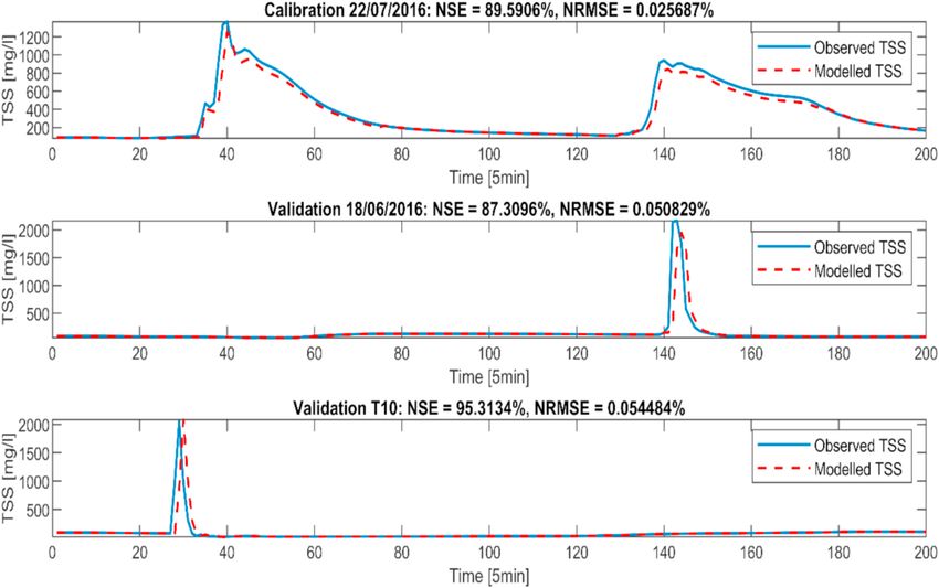
C. Sun et al. Journal of Environmental Management 294 (2021) 113031
simulation such as the Storm Water Management Model (SWMM) based on input and output flows:
(Rossman, 2015), MIKE Urban (DHI, 2017), WaterCress (Clark et al., ( )
∑
nin ∑
nout
2002), InfoWorks CS (MWH, 2010) and UrbanCycle (Hardy et al., 2005). vol(k + 1) = vol(k) + Δt i
fin (k) − i
fout (k) (1)
These models and tools can represent quality dynamics and processes in i=1 i=1
SN. But the tools mainly work as simulation platforms, which may not be
able to use for optimization. The detailed models are not suitable for 0 ≤ f (k) ≤ f max (2)
optimization either due to the high computational requirement.
Control-oriented quality models which can describe complex dy 0 ≤ vol(k) ≤ volmax (3)
namics using simple equations (generally linear) are in need for pollu
tion optimization in real time, especially for large scale SN. Lacour and where vol ∈ Rnt represents vector for the water volumes [m3 ] stored in
Schütze (2011) proposed a turbidity-based approach, which uses detention tanks with physical ranges in [0, volmax ]; Δtis sampling time
turbidity measurements to generate “realistic” signals at the inflow time [s] and k is time step; f in = (fin1 , … finnin ) ∈ Rnin is the vector of flows into
nout
series. This approach provides evidence about the potential of the tank [m3 /s]; f out = (fout
1
, …fout ) ∈ Rnout is the vector of flows out of
max
quality-based control but does not map the quality dynamics inside SN. 3
the tank [m /s]; f is the vector containing physical or operational
Vezzaro et al. (2014) considered relevant water quality indicators (TSS - limitations of flows. The parameters nt , nin , nout are numbers of tanks,
total suspended solids and ammonia concentration) in a global control of inflow and outflow branches, respectively.
urban catchments through a simple model. Water quality is included in
cost functions, which allows to change discharge priority to reduce 2.1.2. Controllable actuators
pollution. However, the quality model does not refer to the sewer The controllable actuators, gates or pumps, are usually located at the
network. Torres-Matallana et al. (2018) developed a simplified inlet or the outlet of a tank or an inline detention element. Flow from
semi-distributed urban water quality model, EmiStatR, to simulate these elements is considered as control variable and bounded by phys
emissions of pollutants in terms of chemical oxygen demand and NH4 ical and operational constraints:
concentrations. However, EmiStatR does not model the quality dy
u(k) ≤ umax (k) (4)
namics in sewer pipe explicitly either.
Under this context, this paper contributes 1) a control-oriented
where u is vector of control variables, umax includes the maximum
quality modelling approach for different elements of SN. The model
constraints.
equations are developed independently for different elements, which
allows scalable use of the models. These models are used to represent
2.1.3. Junction node
complex quality dynamics using simple equations, which can be
Mass balance is used for water in and out of a junction node:
embedded in real time optimization process. As a first step, TSS has been
selected as a relevant quality indicator. This choice takes into account ∑
nout ∑
nin
i
fout (k) = finj (k) (5)
that TSS can usually be correlated with turbidity (Lacour and Schütze, i=1 j=1
2011). Similarly, other quality parameters can also be estimated from
TSS. 2) A calibration procedure based on data produced by a virtual i
where fout
j
, i = 1, …, nout are flows leaving the node; fin , j = 1, …, nin are
reality simulator as well as a sensitivity analysis are presented to vali
flows into the node.
date accuracy of the model. 3) Based on the proposed quality models, a
quality-based optimization approach has been developed using model
2.1.4. Overflow
predictive control (MPC). 4) In order to validate the modeling and
Overflows at CSO locations occur, e.g. by means of weirs, when the
optimization approaches, a real life case study based on the Badalona SN
capacity of a downstream element (for example, the WWTP) is exceeded
in Spain has been demonstrated using different rain scenarios.
by the flow in the upstream element, which is modelled as:
Rest of this paper is organized as follows. In Section 2, the control-
oriented quality modelling approach, the calibration procedure and f cso (k) = max{0, f in (k) − maxcap (k)} (6)
the quality-based optimization scheme are presented. In Section 3, the
proposed models are calibrated using data generated by virtual reality f out (k) = f in (k) − f cso (k) (7)
simulations. The efficient and effectiveness of the modeling and opti
mization approaches are demonstrated through the Badalona SN. Con where f in is the flow vector in the upstream elements, maxcap is the
clusions and discussions are provided in Section 4. capacity vector of the downstream of the weirs (possibly WWTP inlets or
interceptors), f out is the flow vector going to the downstream and f cso is
the CSO vector.
2. Methodology
2.1.5. Total CSO
2.1. Modelling approach
The CSO volume released into the receiving environment is
computed as:
The control-oriented modelling approach is used to estimate TSS
dynamics in a certain horizon, including the TSS transportation in sewer ∑
ncso
pipes, TSS deposition and erosion in a detention tank, as well as TSS fenvironment (k) = i
fcso (k) (8)
dynamics in the intersection nodes. There is no direct mathematical
i=1
association between the models and the physical processes. Each type of where ncso is number of CSO.
element in SN is modelled using separated equations to enhance model Based on these equations, TSS models for different elements in SN are
scalability for different networks. developed as follows:
Basic hydraulic models are provided firstly as background before
introducing the quality models. 2.1.6. TSS model for a sewer
In this paper, the italic bold font is used for vectors, italic font rep A sewer or a collection of sewers in a SN can be assumed as a tank
resents scalars. which collects water based on the volumetric difference between input
and output flows, as presented in equation (1).
2.1.1. Detention tank For the outflow vector f out , besides complying with the physical
A detention tank is considered as container which collects water
2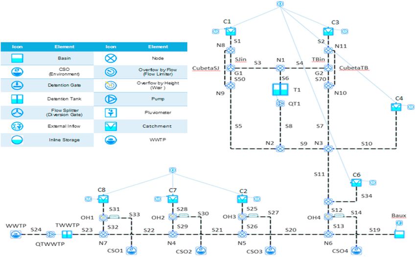
C. Sun et al. Journal of Environmental Management 294 (2021) 113031
constraints of equation (3), the values of f out (k) should also be propor Assuming in the detention tank, TSS is the same throughout the
tional to the sewer volume vol(k) at the current time step k, which can be stored water, which is also TSS at the tank outlets is (valid only for vol >
represented as: 0):
f out (k) = cint vol(k) (9) m(k + 1)
ssout (k + 1) = (14)
vol(k + 1)
where cint is a vector of parameters which relates the outflow of a sewer
with the water volume stored in it. Here cint works as an intermediate 2.1.8. TSS model for a junction node
variable in the modelling process. A junction node is considered as the element where volume and
After combining equations (1) and (9), the following in-out relation suspended solid mass are split or merged based on mass balance. Take a
can be expressed for a hydraulic transport in a sewer: junction of two incoming sewers with one downstream sewer as an
f out (k + 1) = (1 − cint Δt)f out (k) + cint Δt f in (k) (10) example, when suspended solid mass reaches a junction node, the dy
namics of TSS is modelled as:
where the outflow vector f out at time step k + 1 is estimated through
eout (k)ssout (k) = e1in (k)ss1in (k) + e2in (k)ss2in (k) (15)
summing the proportional parts of the outflow vector f out and inflow
vector f in at time step k.
where eout is the coefficient for the TSS output flow, eiin is coefficient for
Taking into account the correlation between TSS dynamics and the
the i-th TSS input flow. They are positive parameters need to be cali
flow rate inside a sewer, similar in-out relation of equation (10) is used
brated in range of [0, 10]. To give the same weight for each coefficient
to generalize the transport model for the TSS inside sewer with co
for the multi-input junction nodes, each coefficient should be close to 1.
efficients c1 and c2 :
ssout (k + 1) = c1 ssin (k) + c2 ssout (k) (11)
2.2. Calibration procedure
where ssout ∈ Rnout is the TSS vector [mg/l] out of a sewer, ssin ∈ Rnin is
TSS vector [mg/l] into a sewer; c1 and c2 are parameters need to be The proposed quality models should be calibrated before application.
calibrated at the range of [0, 1]. A virtual reality simulator of SN is used to produce data sets required by
the calibration process, which has been designed and calibrated based
2.1.7. TSS model for a detention tank on real life plants and measurements. So that the quality processes can
The TSS model in a detention tank is based on a simple representa be represented correctly by the simulator. As described in the modelling
tion of TSS mass evolution considering deposition and erosion processes. approach, water flows, TSS in and out of a sewer are the only infor
According to equation (1), a detention tank has the capacity to collect mation required by the calibration. Different historical rainfall data are
water volume based on input and output flows. Similarly, TSS mass used as inputs to the simulator to generate the required information.
could also be collected in detention tank based on the difference be
tween mass input and output, as well as the deposition and erosion 2.2.1. Calibration for sewer model
phenomena. According to equation (11), c1 , c2 are parameters need to be
Taking m∈ Rnt as the vector of total mass [mg] of the suspended calibrated.
solids in the detained water; ssin and ssout are the TSS vectors for the Defining ss
̂ m as the observed TSS. The observed TSS and flow values
inflows and outflows of a tank; τ as the transport delay happens in the at previous time step are ̂f ,̂ ̂ out . The parameters of c1 , c2 are
̂ in , ss
f , ss in out
mixing process, the evaluation of m in the tank can be presented as: calibrated through minimizing difference between the observed TSS and
m(k + 1) = αm(k) + Δt(f in (k − τ )ssin (k − τ ) − fout (k − τ )ssout (k − τ )) (12) the modelled TSS:
argmin ( )12
/
where α is a vector representing mass deposition and/or erosion pro ∑
N 2
( )
c*1 , c*2 = ( ss
̂ m (k) − c1 ss ̂ out (k − 1))
̂ in (k − 1) − c2 ss (16)
cesses and should be calibrated using values between 0 and 10 for each k=1
(c1 ,c2 )
tank; τ represents non-negative integer of transportation delays. The
values ofα in the range of [0, 1] describes the deposition process while where N is duration of the event.
the values at the range of [1, 10] represents the erosion process. Here the
erosion constraint 10 is only an estimated maximal constraint. Bigger 2.2.2. Calibration for tank model
constraint can be used in real implementations with stronger erosion. In The parameters α, β, γ, τ need to be calibrated for the tank model. The
order to achieve a model with accuracy, the items in equation (12) might sedimentation and erosion phenomena are represented through setting
be modified by considering more independent coefficients: values at different ranges for the calibrated parameters. When the
m(k + 1) = αm(k) + Δtβf in (k − τ )ssin (k − τ ) − Δtγf out (k − τ )ssout (k − τ ) parameter takes value from 0 to 1, it means the sedimentation happens,
when setting values at the range of [1, 10], erosion happens. There may
(13)
have sedimentation and erosion two processes happen together in re
where β, γ are positive vectors to be calibrated for each tank using values ality, however, we consider in this work only one process happens at
between 0 and 10. each time.
According to equations (1), (13) and (14), the parameters of α, β, γ, τ
are calibrated as:
argmin ⎛ ⎛ ⎞2 ⎞12 /
⎜ ∑N
⎜̂ ̂ ̂
αm(k − 1) + βΔt f in (k − τ − 1) ss in (k − τ − 1) − γΔt f out (k − τ − 1) ss out (k − τ − 1)⎟ ⎟
̂ ̂
(α* , β* , γ* , τ * ) = ⎝ ⎝ ss m (k) − ( ) ⎠⎠ (17)
k=1 vol(k − 1) + Δt ̂f in (k − 1) − ̂
f out (k − 1)
(e*out ,e1* ,e2* )
in in
3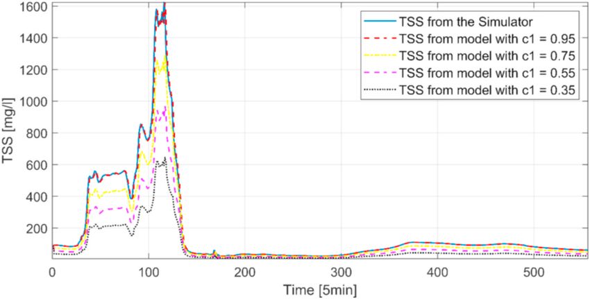
C. Sun et al. Journal of Environmental Management 294 (2021) 113031
information is not readily available. In this case, we do not have reliable
data for the TSS tank model calibration, and we suggest to use an
The initial mass (m(0)) and water volume (vol(0)) at the tank can be approximation of the TSS in detention tank with perfect mixture hy
set as 0 or other initial values read from the simulators. pothesis for the total mass as a conservative alternative. Then, the model
coefficients for the tank model (α, β, γ, τ ) would be (1, 1, 1, 0).
2.2.3. Calibration for junction model
The following equation should be met during calibration while ei and 2.3. Quality-based optimization using MPC
ej takes value from [0 10] but better as close as possible to 1:
argmin
⎛ ⎛ ⎞2 ⎞12/
1 1 2 2
( ) ∑N 1̂ 2̂
e*out , e1* 2* ⎜ ⎜ i e f (k) ss
̂ m (k) − in in
⎝ ss
̂ in (k) + ein f in (k) ss
̂ in (k)⎟ ⎟ (18)
in , ein = ⎝ ⎠⎠
e ̂f out (k)
(e*out 1*
in
2*
,e ,e )
in
k=1 out
MPC has been selected as the optimization scheme because of its
capacity to generate optimal control strategies especially for a complex
network, as proved in García et al. (2015); Joseph-Duran et al. (2015);
2.2.4. Performance evaluation Pleau et al. (2005); Puig et al. (2009); Schütze et al. (2003); and Sun
In order to evaluate the proposed modelling approaches, Nash Sut et al. (2020). The principal goal of the quality-based MPC optimization
cliffe model efficiency coefficient (NSE) (Nash and Sutcliffe, 1970), approach is minimizing both volume and pollutant load of CSO through
which is sensitive to pollutograph peaks, and the Normalized Root Mean efficient operation of controllable actuators (pumps, gates, etc.), taking
Square Error (NRMSE), a standard deviation of prediction errors into account hydraulic and quality models defined previously.
(Functional, 2005) are selected .
2.3.1. Optimization control problems
2.2.4.1. NSE index. Defining average of the observed TSS as ss
̂ m , which The quality-based MPC optimization is defined using a state-space
can be computed as: discrete-time model:
∑N
ss
̂ m (k) minJ(k) (22a)
̂ m = k=1
ss ∑N (19) u(k)
k=1 k
s.t.:
Then performance in terms of NSE for the proposed models can be
computed as: x(k + 1) = f (x(k), u(k), d(k)) (22b)
∑N 2 h(x(k), u(k), w(k)) ≥ 0, (22c)
k=1 (ssout (k) − ss
̂ m (k))
NSEss = 1 − ( )2 (20) g(x(k), u(k), w(k)) = 0, (22d)
∑N
k=1 ss
̂ m (k) − ss
̂ m (k)
xmin ≤ x(k) ≤ xmax , (22e)
The value of NSEss range from − ∞ to 1. If NSEss is equal with 1, it
corresponds to a perfect match of the model. If NSEss can get value umin ≤ u(k) ≤ umax , (22f)
between 0.5 and 0.65, that indicate the model is sufficiently good to be
used (Sun et al., 2017b). where x(k) is state vector represents water volume and mass in all tanks;
u(k) is the controlable vector of gate flows; d(k) is disturbance vector
related to rain intensity and runoff. The functions h(‧) and g(‧) include
2.2.4.2. NRMSE index. The value of NRMSEss is computed using
constraints, umin , umax, xmin , xmax are physical limits of vectors.
equation (21):
√̅̅̅̅̅̅̅̅̅̅̅̅̅̅̅̅̅̅̅̅̅̅̅̅̅̅̅̅̅̅̅̅̅̅̅̅̅̅̅̅̅̅̅̅̅̅̅̅̅̅
√
√
( )2 2.3.2. Objective function
√
2
√∑ N ss out (k) − ss
̂ m (k) The objective function is a mathematical representation of the
1
NRMSEss = ( ) ( )√ operational goals, including CSO discharges minimization Jcso (k),
N
max SŜ m (k) − min SS
̂ m (k) k=1 pollutant loads (TSS mass) from CSO minimization Jm (k) and WWTP
usage maximization Jwwtp , expressed as:
(21)
∑
N
[ ]
In general, is expressed as a percentage, where the lower value J(k) = acso Jcso (k) + am Jm (k) + awwtp Jwwtp (k) (23)
indicate less errors. k=1
2.2.5. Practical implementation where acso , am , awwtp are weights of different objectives which can be
Water quality measurements inside the SN or appropriate estima generated through Pareto front computation for the multi-objective
tions are indispensable for model calibration. For sewer elements, these optimization problem in (23) or in practice, priorities of these items
data may be estimated using a number of real turbidity sensors, com are mainly manipulated by the system operators in order to adjust to
plemented by TSS estimations of a detailed model. For the case of different situations (Lund et al., 2018; Toro et al., 2011).
detention tanks, TSS measurements or estimations at the tank inlet and
output are required. The sensors for the tank inlet and output may not be
available in the real system and in the detailed quality simulators, this
4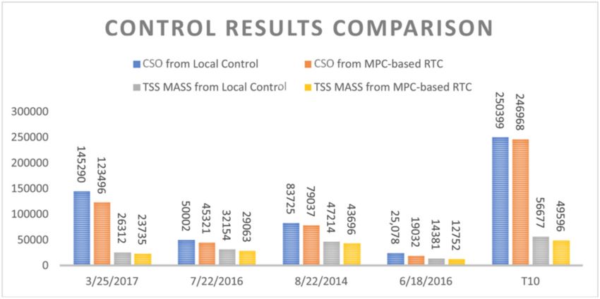
C. Sun et al. Journal of Environmental Management 294 (2021) 113031
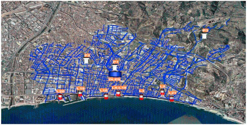
Fig. 1. The Badalona SN.
2.3.3. Control optimization setup
Table 1
The quality-based MPC optimization produces control actions inside
Rain events.
the prediction horizon of H, however, only the first solution is applied
into simulation as set-points to validate the control actions without RAIN I20 I60 START END PREVIOUS RAIN
EVENT TIME TIME DRY DAYS INTENSITY
disturbing the real plant. In order to compensate uncertainty produced
by the conceptual models, in each time step, the new system state (e.g. 25/03/ 39.6 24.6 08:20 06:35 20 Medium
2017 24/03 26/03
the tank volume, mass, etc.) of simulator is used as initial values for the
22/07/ 31.5 18.3 08:25 21:45 53 Small
next step optimization using MPC. This interaction between the 2016 22/07 23/07
controller and simulator is the so called closed-loop optimization 22/08/ 42.6 17.8 09:30 22:30 20 Big
scheme, which has been explained in detail in (Romero-Ben et al., 2019; 2014 22/08 23/08
Sun et al., 2015). 18/06/ 60.3 24.4 03:40 16:25 20 Very big
2016 18/06 19/06
T10 110.5 52.9 00:00 03:00 10 Strong
3. Case study 01/01 02/01
3.1. Badalona sewer network
shown in Fig. 1, the Badalona SN (blue color) includes one detention
Badalona is a city at the east of Catalonia (Spain) facing to the tank (blue cylindrical). The WWTP is located on the side of the coast.
Mediterranean Sea. Affected by the Mediterranean climate, 50% of the Along the coast locates the outfall points (red color) from where the
rainfall occurs at two or three heavy rainfall events in summer and CSOs are released. Three rain gauges P1, P2, P3 are distributed in
autumn, which used to generate CSOs to the beach of Badalona. As different area of this network.
Fig. 2. Simplified Badalona SN.
5
C. Sun et al. Journal of Environmental Management 294 (2021) 113031
The Badalona SN has been simulated in InfoWorks Integrated results of this calibrated model using rainfalls 18/06/2016 and T10,
Catchment Modelling (InfoWorks ICM) (MWH, 2010). Full 1D Saint where more than 85% NSE fitting accuracies are still achieved, the
Venant equations (Joseph-Duran et al., 2014a) is used in InfoWorks to NRMSE errors are less than 0.01%, as shown in Fig. 3 as well.
solve the hydraulic dynamics. Velikanov model (Zug et al., 1998) is used Table 2 presents more details about the calibration and validation
to describe dynamics of TSS in a detention tank. The TSS in the sewer is results, which includes the calibrated parameters and performance in
linear and instantaneous. each case. Considering both the calibration and validation performance
To compute the quality-based MPC optimization, the Badalona SN in NSE are better than 80%, the NRMSEs are less than 0.1%, the pro
has been conceptualized as Fig. 2 with a clear layout includes 7 catch posed TSS model for the sewer can represent the TSS dynamics well at
ments (C1, C2, C3, C4, C6, C7, C8) and a basin (Baux) connected by 35 the Badalona pilot.
links and 5 outfalls. There are 2 gates (G1, G2) operate water input to the Considering the fact that, there exists uncertainties for using con
detention tank, one pump station (QT1) to empty the detention tank and ceptual models. In order to get a better knowledge about the uncertainty
another pump (QTWWTP) to schedule flows towards the WWTP. The influence, sensitivity analysis is carried out. The following steps are
conceptualization process can be found in (Martínez et al., 2019). applied into analysis, which firstly fix c1, and add c2 with 0.02, 0.04,
0.06 individually; then fix c2, and minus c1 with 0.2, 0.4, 0.6 separately,
3.2. Quality modelling calibration considering the different order of magnitude in c1 and c2. Fitting results
are provided with 25/03/2017 as representative scenario. The results at
To generate calibration data from the simulator, 4 real rain events Figs. 4–5 show that the uncertainty of c1 which is coefficient of the TSS
and a synthetic scenario T10 have been applied (Table 1). The real input at the previous time step, affects more about the TSS sewer than
rainfall was measured in terms of 5-min interval from the year the coefficient of the previous TSS output c2. Furthermore, higher in
2014–2017. The selected rains are the representative events with tensity rainfall period is affected more when modifying the calibration
different characteristics (small, medium, big, very big). The synthetic parameters. However, the trends of the curves can always be captured.
scenario T10 was designed as a strong rainfall of 10-year return period
following a rainfall distribution prepared by Alternating Block Method 3.2.2. Model for junction node
(Ghazavi et al., 2017). In Table 1, start and end time of the rain are in The junction node model is validated through a downstream node
format of HH:MM DD/MM. Previous dry days are given for each sce N6 of the Badalona SN, which has two input branches S13, S19 and one
nario. Moreover, I20 , I60 which represent precipitation intensities output S20 according to equation (19):
considering 20-min and 60-min time steps are provided to describe the 13 13 19
intensity. e1in ̂f in (k) ss
̂ in (k) + e2in (k) ss
̂ in (k)
̂ 20
ss m (k) = 20
(24)
eout ̂f out (k)
3.2.1. Model for sewer
Regarding the coefficient constraints, for the node N6, the optimal
To illustrate the TSS sewer model, the sewer S2 (as shown in Fig. 2) is
calibrated value for e1in , e2in and eout are near 1, which represents sus
selected as an example to calibrate the proposed sewer model. Among
pended solids at the junction node follow mass balance.
the 5 rain events, the first three of them (25/03/2017, 22/07/2016, 22/
Fig. 6 list the calibration results of N6 based on the 22/07/2016,
08/2014) are used for calibration, while the rest two events (18/06/
where the TSS output for the S20 computed from the model (15) is quite
2016, T10) are used for validating the models produced by the
similar with the observed one from simulator using the value of 1 for e1
calibration.
and e2 . The result confirms that, the suspended solids in the junction
Fig. 3 includes the calibration result of S2 for the rain event 22/07/
node N6 fits well mass balance equation with very few deviations at the
2016, which has more than 89% NSE fitting accuracy. The NRMSE index
Badalona pilot.
is less than 0.03%, which indicates very few errors. The validation
Fig. 3. Calibration and validation results.
6
C. Sun et al. Journal of Environmental Management 294 (2021) 113031
Table 2
Calibration and validation results.
CALIBR./VALID. C2 C1 NSE NRMSE 18/06/2016 T10
25/03/2017 0.04 0.95 93% 0.02% 87% 0.05% 95% 0.05%
22/07/2016 0.08 0.99 90% 0.03% 86% 0.04% 93% 0.07%
22/08/2014 0.08 0.90 76% 0.04% 88% 0.03% 94% 0.06%
Fig. 4. Sensitivity Analysis for rainfall 25/03/2017 when fixes c2 as constant. Fig. 7. Control results comparison in terms of CSO and TSS MASS (m3).
Table 4
Optimizer and simulator configuration.
GAMS Optimizer InfoWorks Simulator
# variables 970 # nodes 14,285
# equations 981 # links 15,055
#compute time 1.32s 31.31s
#CPU
3.3. Optimal control application
In order to demonstrate effectiveness of the proposed quality
modelling approaches, quality-based optimization approach using MPC
Fig. 5. Sensitivity Analysis for rainfall 25/03/2017 when fixes c1 as constant. is applied. In each iteration, MPC optimizes the defined objective
function at equation (23) using the proposed quantity and quality
equations to produce optimal operation strategies for the Badalona pilot.
The GAMS optimization library (Rosenthal, 2013) is used as a solver.
The quality-based optimization approach has been validated using
rain episodes of 25/03/2017, 22/07/2016, 22/08/2014, 18/06/2016
and a synthetic scenario T10. The calibration results for the quality
models listed in Table 3 are used. The optimization results in items of
CSO and TSS mass are compared with the ones produced by Local Control
strategies which generate operation actions based on a set of predefined
rules regarding hydraulic measurements.
Fig. 7 provides the CSO volume and mass comparisons between Local
Control and MPC-based optimization under different rainfall events. The
results confirm that, both CSO volume and mass pollution released to the
environment are reduced after considering a MPC-based optimization
Fig. 6. Junction model calibration for N6 at rain 22/07/2016. with quality models. For some rain scenarios, more than 20% CSO
reduction and more than 12% TSS pollution are reduced, which repre
sent a significant improvement for the receiving water and environment.
Table 3 Furthermore, considering the optimization results are affected a lot by
Quality models used in RTC application. the network topology as well as the rainfall intensity, a more noticeable
RAIN RAIN INTENSITY C2 C1 α β γ τ difference between the volume-based strategies and the quality-based
EVENT one might be observed in scenarios with very different quality indica
25/03/2017 Medium 0.04 0.95 1 1 1 0 tor values at the tank inlets. Similarly, in network configurations with
22/07/2016 Small 0.08 0.99 more detention tanks and/or actuators, more degrees of optimization
22/08/2014 Big 0.08 0.90 and large improvement potentials exist for quality-based MPC
18/06/2016 Very big 0.11 0.89
T10 Strong 0.01 0.99
optimization.
To confirm that add quality models into optimization can still meet
real-time requirements, Table 4 summarizes computation loads for both
the controller and simulator:
7C. Sun et al. Journal of Environmental Management 294 (2021) 113031
It is clear that the mean computation time of one step optimization is simplified models; the Closed-loop Simulation Framework software; and
much smaller than one step simulation, which make real-time optimi the rain data) and Innovyze (for licenses to InfoWorks ICM). Also
zation possible, also in a large scale network. appreciate for the support from NWO (Netherlands Organisation for
Scientific Research) Sectorplan for Beta and Technology Programme in
4. Conclusion and discussion Wageningen University.
This work proposed a control-oriented quality modelling approach References
for TSS in SN, which open up new potential for optimization of pollution
load from CSO in large scale network in real time. The calibration and Becouze, C., Bertrand-Krajewski, J.-L., Dembélé, A., Cren-Olivé, Coquery, M., 2009.
Preliminary assessment of fluxes of priority pollutants in stormwater discharges in
validation results in the Badalona SN confirms applicable of the models two urban catchments in Lyon, France. In: Proceedings of the 13th IWA International
in a realistic and accurate way from all the available sources (more than Conference on Diffuse Pollution and Integrated Watershed Management, p. 10.
80% NSE and less than 0.1% NRMSE). The sensitivity analyze for the TSS Seoul, South Korea).
Cembrano, G., Quevedo, J., Salamero, M., Puig, V., Figueras, J., Martí, J., 2004. Optimal
model in a sewer shows that the TSS input coefficient affects more than control of urban drainage systems, A case study. Contr. Eng. Pract. 12 (1), 1–9.
the coefficient of the previous TSS output. The peak time with higher https://doi.org/10.1016/S0967-0661(02)00280-0.
intensity rainfall period is more likely to be affected with more inac Clark, R., Pezzaniti, D., Cresswell, D., 2002. Watercress—community Resource
Evaluation and Simulation System—a tool for innovative urban water system
curacy. This peak time cannot be managed from the sediment transport planning and design. In: Proceedings of the 27th Hydrology and Water Resources
formulas because it is related to the hydraulic behavior (where a peak Symposium, p. 870. Melbourne, Australia.
time difference also exists). To improve the models, much more real data Dhi Danish Hydraulic Institute, 2017. Mike urban. https://www.mikepoweredbydhi.
com/products/mike-urban.
to accurately calibrate TSS behavior is needed. Moreover, online sensors EPA, 2015. Wastewater Management: Controlling and Abating Combined Sewer
are also advised to properly capture the TSS evolution in wet weather. Overflows. Inspector General Evaluation Report. Washington D.C, USA. http
A quality-based MPC optimization is also presented after considering s://www.epa.gov/sites/production/files/2015-12/documents/csofinal.pdf.
Fu, G., Khu, S.T., Butler, D., 2010. Optimal distribution and control of storage tank to
both the quality and hydraulic models. Comparing with the current local
mitigate the impact of new developments on receiving water quality. J. Environ.
control, in some rain scenarios, the quality-based MPC optimization Eng.-ASCE 136 (3), 335–342. https://doi.org/10.1061/(ASCE)EE.1943-
approach can achieve more than 20% reduction in CSO volume and 7870.0000161.
more than 12% TSS reduction in released pollution. The potential Fu, B., Horsburgh, J.S., Jakeman, A.J., Gualtieri, C., Arnold, T., Marshall, L., et al., 2020.
Modeling water quality in watersheds: from here to the next generation. Water
improvement of the optimization approach could be different in Resour. Res. 56 https://doi.org/10.1029/2020WR027721 e2020WR027721.
different pilots. The considered quality indicators, the available mea Functinoal Networks, 2005. Functional Equations in Applied Sciences, pp. 169–232.
surements, magnitudes of CSOs, intensity of rainfalls, as well as the https://doi.org/10.1016/s0076-5392(05)80012-8.
García, L., Barreiro-Gomez, J., Escobar, E., Télleza, D., Quijanoa, N., Ocampo-
physical topology of the network can all affect the application effec Martinez, C., 2015. Modeling and real-time control of urban drainage systems: a
tiveness. To get better optimization results, more integration with other review. Adv. Water Resour. 85, 120–132. https://doi.org/10.1016/j.
catchments and treatment plants in the watershed from a global advwatres.2015.08.007.
Ghazavi, R., Rabori, A.M., Reveshty, M.A., 2017. Effects of rainfall intensity-duration-
perspective, or even with the supply network should provide more frequency curves reformation on urban flood characteristics in semiarid
possibilities and potentials. environment. Ecopersia 5 (2), 1801–1815. https://doi.org/10.18869/modares.
Ecopersia.5.2.1801.
Hardy, M.J., Kuczera, G., Coombes, P.J., 2005. Integrated urban water cycle
5. Credit author statement management: the UrbanCycle model. Water Sci. Technol. 52 (9), 1–9. https://doi.
org/10.2166/wst.2005.0276.
Congcong Sun: Conceptualization, Methodology, Investigation, Hoppe, H., Messmann, S., Giga, A., Gruening, H., 2011. A real-time control strategy for
separation of highly polluted storm water based on UV-Vis online measurements -
Validation, Original draft preparation, Reviewing and Editing; Luis from theory to operation. Water Sci. Technol. 63, 2287–2293. https://doi.org/
Romero Ben: Software, Writing- Reviewing and Editing; Eduard Muñoz 10.2166/wst.2011.164.
Craviotto: Software, Reviewing and Editing. Vicenç Puig: Methodology, Joseph-Duran, B., Ocampo-Martínez, C., Cembrano, G., 2014a. Hybrid modelling and
receding horizon control of sewer networks. Water Resour. Res. 50 (11), 8497–8514.
Supervision, Reviewing and Editing. Bernat Joseph-Duran, Jordi Mese https://doi.org/10.1002/2013WR015119.
guer, Gabriela Cembrano, Montse Martinez and Puentes Ramon Guasch Joseph-Duran, B., Jung, M.N., Ocampo-Martinez, C., Sager, S., Cembrano, G., 2014b.
Palma: Methodology, Supervision, Reviewing and Editing, Project Minimization of sewage network overflow. Water Resour. Manag. 28, 41–63.
https://doi.org/10.1007/s11269-013-0468-z.
administration, Funding acquisition.
Joseph-Duran, B., Ocampo-Martínez, C., Cembrano, G., 2015. Output-feedback control of
combined sewer networks through receding horizon control with moving horizon
estimation. Water Resour. Res. 51 (10), 8129–8145. https://doi.org/10.1002/
Declaration of competing interest 2014WR016696.
Lacour, C., Schütze, M., 2011. Real-time control of sewer systems using turbidity
measurements. Water Sci. Technol. 63 (11), 2628–2632. https://doi.org/10.2166/
The authors declare that they have no known competing financial
wst.2011.159.
interests or personal relationships that could have appeared to influence Ledergerber, J.M., Maruéjouls, T., Vanrolleghem, P.A., 2019. Optimal experimental
the work reported in this paper. design for calibration of a new sewer water quality model. J. Hydrol 574,
1020–1028. https://doi.org/10.1016/j.jhydrol.2019.05.004.
Lund, N.S.V., Falk, A.K.V., Borup, M., Madsen, H., Mikkelsen, P.S., 2018. Model
Acknowledgement predictive control of urban drainage systems: a review and perspective towards
smart real-time water management. Crit. Rev. Environ. Sci. Technol. 48 (3),
279–339. https://doi.org/10.1080/10643389.2018.1455484.
The authors wish to acknowledge the support from the European Maciejowski, J.M., 2002. Predictive Control with Constraints. Prentice Hall, Bergen, New
Commission research grant of project LIFE EFFIDRAIN (LIFE14 ENV/ Jersey, USA.
ES/000860), from Spanish national project DEOCS (DPI2016-76493-C3- Martínez, M., Guasch, R., Ruiloba, L.C., Craviotto, E.M., Cembrano, G., Sun, C.C., 2019.
D9 mediterranean pilot set-up and demonstrator configuration. Deliverable of LIFE
3-R) and the internal project TWINs from the CISC (Spanish State
EFFIDRAIN project. http://www.life-effidrain.eu/uploads/pdf/cf7909da
Research Agency) through the María de Maeztu Seal of Excellence to IRI 58070904aa99ad1b98e18e3f.pdf.
(MDM-2016-0656). The authors also thank Aigües de Barcelona for their Mwh, 2010. InfoWorks CS. Innovyze. Newbury, UK. http://www.innovyze.com/pro
financial and technical support. Considering the fact that data, models ducts/infoworks_cs/.
Nash, J.E., Sutcliffe, J.V., 1970. River flow forecasting through conceptual models part I-
and tools used in this research are confidential or commercial, we refer A discussion of principles. J. Hydrol 10 (3), 282–290. https://doi.org/10.1016/
other researchers to contact SUEZ Spain Group (for access to detailed, 0022-1694(70)90255-6.
8C. Sun et al. Journal of Environmental Management 294 (2021) 113031
Pleau, M., Colas, H., Lavallée, P., Pelletier, G., Bonin, R., 2005. Global optimal real-time models. In: Proceedings of the 14th IWA/IAHR International Conference on Urban
control of the Quebec urban drainage system. Environ. Model. Software 20 (4), Drainage, pp. 1848–1855. Prague, Czech Republic.
401–413. https://doi.org/10.1016/j.envsoft.2004.02.009. Sun, C.C., Joseph-Duran, B., Maruejouls, T., Cembrano, G., Meseguer, J., Puig, V.,
Puig, V., Cembrano, G., Romera, J., Quevedo, J., Aznar, B., Ramón, G., Cabot, J., 2009. Litrico, X., 2017b. Real-time control-oriented quality modelling in combined urban
Predictive optimal control of sewer networks using CORAL tool: application to Riera drainage networks. In: Proceedings of the 20th IFAC World Congress, pp. 3941–3946.
Blanca Catchment in Barcelona. Water Sci. Technol. 60 (4), 869–878. https://doi. https://doi.org/10.1016/j.ifacol.2017.08.142. Toulouse, France.
org/10.2166/wst.2009.424. Sun, C.C., Joseph-Duran, B., Cembrano, G., Puig, V., Meseguer, J., 2018. Advanced
Romero-Ben, L., Sun, C.C., Guasch-Palma, R., Joseph-Duran, B., Meseguer, J., integrated real-time control of combined urban drainage systems using MPC:
Cembrano, G., Puig, V., 2019. A feedback simulation procedure for real-time control Badalona case study. In: Proceedings of the 13th International Conference on
of urban drainage systems. In: Proceedings of the 1st IFAC Workshop on Control Hydroinformatics, pp. 2033–2041. https://doi.org/10.29007/27gp. Palermo, Italy.
Methods for Water Resource Systems, vol. 52, pp. 101–106. https://doi.org/ Sun, C.C., Romero, L.B., Joseph-Duran, B., Meseguer, J., Craviotto, E.M., Guasch, R.P.,
10.1016/j.ifacol.2019.11.016 (23) Delft, The Netherlands. Martinez, M.P., Puig, V., Cembrano, G., 2020. Integrated pollution-based real-time
Rosenthal, R., 2013. GAMS – A User’s Guide. GAMS Development Corporation. control of sanitation systems. J. Environ. Manag. 269, 110798. https://doi.org/
http://www.gams.com/help/topic/gams.doc/userguides/GAMSUsersGuide.pdf. 10.1016/j.jenvman.2020.110798.
Rossman, L., 2015. Storm Water Management Model Users’ Manual Version 5.1. Toro, R., Ocampo-Martinez, C., Logist, F., Van Impe, J., Puig, V., 2011. Tuning of
Environmental Protection Agency, Washington DC, USA. predictive controllers for drinking water networked systems. In: Proceedings of the
Schütze, M., Campisano, A., Colas, H., Vanrolleghem, P., Schiling, W., 2003. Real-time 18th IFAC Proceedings Volumes, vol. 44, pp. 14507–14512. https://doi.org/
control of urban water systems. In: Proceedings of the International Conference on 10.3182/20110828-6-IT-1002.00415 (1) Milano, Italy.
Pumps, Elctromechanical Devices and Systems Applied to Urban Water Torres-Matallana, J.A., Leopold, U., Klepiszewski, K., Heuvelink, G.B.M., 2018.
Management, pp. 1–19. Valencia, Spain. EmiStatR: a simplified and scalable urban water quality model for simulation of
Schütze, M., Campisano, A.C., Colas, H., Schilling, W., Vanrolleghem, P.A., 2004. Real combined sewer overflows. Water 10, 782. https://doi.org/10.3182/10.3390/
time control of urban wastewater systems - where do we stand today? J. Hydrol 299 w10060782.
(3–4), 335–348. https://doi.org/10.1016/j.jhydrol.2004.08.010. Vezzaro, L., Christensen, M.L., Thirsing, C., Grum, M., Mikkelsen, P.S., 2014. Water
Sun, C.C., Puig, V., Cembrano, G., 2015. Integrated simulation and optimization scheme quality-based real time control of integrated urban drainage systems: a preliminary
of real-time large-scale water supply network: applied to Catalunya case study. study from Copenhagen, Denmark. Procedia Eng. 70, 1707–1716. https://doi.org/
Simulation 91 (1), 59–70. https://doi.org/10.1177/0037549714559982. 10.1016/j.proeng.2014.02.188.
Sun, C.C., Joseph-Duran, B., Maruejouls, J., Cembrano, G., Muñoz, E., Meseguer, J., Zug, M., Bellefleur, D., Phan, L., Scrivener, O., 1998. Sediment transport model in sewer
Montserrat, A., Sampe, S., Puig, V., Litrico, X., 2017a. Efficient integrated model networks – a new utilization of the Velikanov model. Water Sci. Technol. 37 (1),
predictive control of urban drainage systems using simplified conceptual quality 187–196. https://doi.org/10.2166/wst.1998.0046.
9You can also read