The duration energy size enigma for acoustic emission - Nature
←
→
Page content transcription
If your browser does not render page correctly, please read the page content below
www.nature.com/scientificreports
OPEN The duration‑energy‑size enigma
for acoustic emission
Blai Casals1*, Karin A. Dahmen2, Boyuan Gou3, Spencer Rooke2 & Ekhard K. H. Salje1
Acoustic emission (AE) measurements of avalanches in different systems, such as domain movements
in ferroics or the collapse of voids in porous materials, cannot be compared with model predictions
without a detailed analysis of the AE process. In particular, most AE experiments scale the avalanche
energy E, maximum amplitude Amax and duration D as E ~ Amaxx and Amax ~ D χ with x = 2 and a
poorly defined power law distribution for the duration. In contrast, simple mean field theory (MFT)
predicts that x = 3 and χ = 2. The disagreement is due to details of the AE measurements: the initial
acoustic strain signal of an avalanche is modified by the propagation of the acoustic wave, which
is then measured by the detector. We demonstrate, by simple model simulations, that typical
avalanches follow the observed AE results with x = 2 and ‘half-moon’ shapes for the cross-correlation.
Furthermore, the size S of an avalanche does not always scale as the square of the maximum AE
avalanche amplitude Amax as predicted by MFT but scales linearly S ~ Amax. We propose that the AE rise
time reflects the atomistic avalanche time profile better than the duration of the AE signal.
Avalanches commonly occur during deformation and failure of materials1–25. They dominate the hysteretic
behaviour of domain switching in electric, magnetic or strain fields. They also occur in scenarios where local
restructuring occurs, such as the collapse of voids in porous materials. Here we focus on ferroic switching as the
defining feature that contributes to the classic Barkhausen noise26–31. The energy of avalanches in Barkhausen
noise is partially released by elastic waves during acoustic emission, AE. As AE measurements have unsurpassed
sensitivity they became the method of choice for the investigation of field induced changes in ferroics and are
hence at the heart of current research into the dynamics of switching processes2,13,14,17–22,30,32–36. Here we show
why some results of AE deviate from the predictions of mean field theory, M FT14,37.
The following parameters are typically measured during AE experiments: the energy E of an avalanche, the
time evolution of the AE amplitudes AAE(t), the maximum AE amplitudes Amax per avalanche, their duration D
and various correlations between avalanches like waiting time, aftershocks38 etc.… Other parameters are obtained
indirectly, like the size S by integrating |AAE(t)| over time t during the progression of the avalanche. The funda-
mental assumption is then that these quantities can be equated with the fundamental avalanche parameters (i.e.
of the behaviour of the avalanche source). These parameters are E, V(t), Vmax, and duration T. Similarly, the size
S is derived from model simulations by integration over V(t), this function can then be compared with the AE
size function. We use the common nomenclature of the AE literature and add a subscript AE whenever there is
a danger that the reader confuses the quantities of the AE experiment and the equivalent (atomistic) avalanche
parameter. The non-equivalence between EAE and E, AAE(t) and V(t), Amax and Vmax, and the AE duration D and
its equivalent duration T of the atomic avalanche is at the heart of this study.
The amplitude AAE(t) is an experimental quantity directly measured in an AE experiment, namely the ampli-
tude of the strain wave arriving at the AE detector (Fig. 1). The local process of the avalanche nucleation and
progression produces local strain amplitudes which is denoted A(t). A(t) is the local strain amplitude at the time
t and represents the change of the atomic configuration at time t. It hence represents a ‘rate of change’ which
we call in this paper V(t). The atomic interpretation of V(t) as ‘velocity’ of the advancing front of an avalanche
is appropriate if the avalanche is a fairly compact region while nucleation and fractal regions do not have such
a simple geometrical interpretation. In these cases, V(t) is understood as a ‘displacement rate’ when the objects
are spatially distributed or fractal. In accordance with convention, we still use the symbol V(t) bearing in mind
this more general ‘rate’ definition. In particular, the relevant patterns in ferroics are extremely complex and only
occasionally compact. We use the symbol V(t) with the understanding that V(t) does not just mean a simple
front propagation as, e.g., described in the Avrami–Ishibashi approach39,40.
The analysis of AE spectra is typically based on their comparison with model s imulations4–7,12,14,18,19,23. Most
model parameters were initially borrowed from research into Earth Quake statistics [e.g. 41] so that the
1
Department of Earth Sciences, Cambridge University, Cambridge, UK. 2Department of Physics, University of
Illinois, Urbana, IL 61801, USA. 3State Key Laboratory for Mechanical Behavior of Materials, Xi’An Jiao Tong
University, Xian 710049, Shaanxi, People’s Republic of China. *email: blaicasals@gmail.com
Scientific Reports | (2021) 11:5590 | https://doi.org/10.1038/s41598-021-84688-7 1
Vol.:(0123456789)
www.nature.com/scientificreports/
Figure 1. Schematic representation of the composition of an avalanche signal in acoustic emission experiments.
The size of the sample and the detector is some 5 mm, the detector covers often a large part of the sample.
During local switching, an avalanche with V(t) emits a strain signal (i.e. the source function) which propagates
through the sample and is eventually measured by the detector. During the propagation, the signal generates the
ringing of the sample and is modified by elastic wave reflections on surfaces, scattering on lattice imperfections.
The profile of a source delta function would generate T(t), the so-called transfer function. The measured AE
profile AAE(t) is described in this paper as the convolution of the source function with the transfer function.
nomenclature was historically taken from this field. The fingerprint for critical avalanches is that the probability
distribution functions (PDF) of EAE, Amax, and D are power law distributed with exponents ε, τ′, and α, respec-
DAE
tively. Here the energy is derived from the AE spectrum of AAE(t) by EAE = ∫ AAE (t)2 dt . Correlations exist
0
between these parameters which also follow power laws with EAE ~ Amaxx and Amax ~ DAEχ30.
Experimentally, the power law exponents ε and τ′ are typically measured over many decades and our knowl-
edge of any systematics of the dynamic properties of energies and amplitudes is rather good. The same is not true
for the duration D. There are very few AE measurements available to determine α with reasonable a ccuracy17,42,43.
The PDF of the duration D often follows a power law in some approximation for long durations, while it shows
either constant or exponential distributions for short durations. ‘Half-moon’ shapes are found when plotting the
durations as function of the maximum amplitudes, D(Amax), and duration as function of the avalanche energy,
D(E)17,30,44. As the integration to determine EAE covers the duration of the AE signal, the correlation between
the energy EAE and the maximum amplitude of an avalanche Amax as described by the correlation exponent x,
is equally enigmatic.
The enigma, which we address in this paper, is the scaling between the AE energy and the AE maximum
amplitude EAE ~ Amaxx. This relation is often the starting point for further analysis of the avalanche mechanism.
Experimentally, x = 2 is found in systems that contain distributions of domain movements that are otherwise
consistent with MFT. AE measurements for BaTiO330 are a key example for x = 2 while x = 3 would be consistent
with MFT simulations. To the best of our knowledge, only the exponent x = 2 has been reported in AE experi-
ments. Exponents x = 3 or intermediate values between 2 and 3 were discussed, but not observed experimentally,
by Vives et al.41. These authors clearly identified the discrepancy between x = 2 and x = 3 but offered no reason. We
rationalize this observation and argue that avalanche exponents are modified by details of the AE e xperiments45.
The characteristic parameters for the energy (E), maximum amplitude (Amax), size (S), duration (D) and rise
time (R) are evaluated by the following definitions from the time evolution of the �(t) signals (the so-called ‘jerk
spectrum’, this terms is used both for AE spikes and also for atomic avalanche anomalies) which hence becomes
V(t) before the convolution and AAE(t) after the convolution :
Amax = max(|�(t)|) (1)
D = t(|�(t → tn )| > �th ) (2)
where th is a threshold of �(t) and tn is the waiting time.
R = t(|�(t)| = Maximum) (3)
D
E = ∫ �(t)2 dt (4)
0
Scientific Reports | (2021) 11:5590 | https://doi.org/10.1038/s41598-021-84688-7 2
Vol:.(1234567890)
www.nature.com/scientificreports/
D
S = ∫ |�(t)|dt. (5)
0
The PDFs of these magnitudes are power laws (e.g. for energy PDF(E) ∼ E −ε). Here we use the exponent ε for
E , τ ′ for Amax , τ for S , α for D and ρ for R . The correlations between these magnitudes are defined as E ∼ Axmax ,
γ
S ∼ Amax , Amax ∼ Dχ and Amax ∼ Rξ.
Sample ringing and average avalanche profile
AE spectroscopy is characterised by a close proximity of the sample and the detector. Both have very similar
dimensions and are closely coupled. It appears impossible to analyse an emitted wave profile, as sometimes done
in geophysics and other acoustic investigations of large bodies, by either inverse or direct m ethods46. Instead,
we consider in this paper a simple approach to estimate the influence of wave propagation on the scaling of the
typical AE parameters. We cannot investigate the actual waveform of the triggering event nor do we analyse
the sample-shape dependence of the AE signal, still we derive a simple interpretation of the AE scaling x = 2.
We first consider acoustic emission of a ferroic material that originates from the propagation of domain
boundaries and domains during s witching30. When domain walls hit the sample surface or when domain walls
intersect or annihilate, they emit a primary strain signal that incites the traveling acoustic wave. Similarly,
crack propagation47,48 and porous c ollapse17,19 generate equivalent AE signals. The signals are then measured
by acoustic detectors and analysed electronically. The key characteristic of AE is that it does not measure the
acoustic collision directly but measures the macroscopic vibration (the so-called ringing) of the sample. Such
ringing phenomena in the 104–107 Hz region were thoroughly investigated in the field of acoustic resonance
spectroscopy49–55. The frequency of the ringing is determined by the elasticity of the sample and is only weakly
influenced by the acoustic wave emitted by the domain switching process.
In order to demonstrate the modifications of the initial source function we first consider a simple toy model.
We use the theoretical averaged source function V(t) which would be measured if the time resolution of the
experiment were extremely poor. In this case, many local events overlap and initiate the ringing of the sample.
This approach has the advantage to clarify the various parameters analytically; a full simulation is presented in
the next paragraph. We use the averaged source function37,56 with the time variable t
2
V(t) = ate−bt (6)
The maximum amplitude Amax of the source signal V(t) scales with parameters a and b as,
1
Amax ∼ ab− 2 (7)
and the rise time called when the maximum amplitude is reached
1
t|Amax ∼ b− 2 (8)
The size of the avalanche is defined as
+∞
S = ∫ |V (t)|dt ∼ a/b (9)
0
The traveling wave is then approximated by the convolution of the source signal with the transfer function.
This convolution is expressed by the integral
+∞
AAE (t′ ) = ∫ V (t)T t ′ − t dt (10)
0
This integral extends over the full time, which in an experimental situation means the full duration of the
source function. We tested several transfer functions (see supplemental material section 1). In our toy model
we use a exponentially damped sinusoidal which is compatible with typical experimental AE p rofiles42,45,57,58:
T(t) = cos (wt)e−qt (11)
where w is the frequency and q is a damping parameter. Figure 3a shows the source function and its convolution
with the transfer function. We also explored a Gaussian decay (supplementary information section 1 and 3)
which is often used to describe resonance ultrasound spectroscopy (RUS) s ignals59, the convolution shows very
similar behaviour to the simple exponential decay.
The source function is parameterised by the non-universal constants a and b denoting the amplitude and the
position of the maximum (i.e. the width of the distribution), respectively. A typical example for the variation of
the source function depending on its width is shown in Fig. 2a, b. The energy E is calculated as the integral over
the squared temporal amplitude.
+∞ +∞ 2
E = ∫ V (t)2 dt = ∫ a2 t 2 e−2bt dt
0 0
√ 2
(12)
2a +∞ 3
2 −1
3
= 3 ∫ u e−u du ∼ a2 b− 2
8b 2 0
Scientific Reports | (2021) 11:5590 | https://doi.org/10.1038/s41598-021-84688-7 3
Vol.:(0123456789)
www.nature.com/scientificreports/

                                                                                                                                                      2
                                            Figure 2.  Scaling relations for the averaged source function. Shapes of source functions V(t) = ate−bt with
                                            different parameters a (a) and b (b), as shown, a changes the amplitude and b modifies both duration and
                                                                                                                                       γ
                                            amplitude. Panels (c–f) show scaling relations before convolution for E ∼ Axmax (c), S ∼ Amax(d), Amax ∼ Dχ(e)
                                            and Amax ∼ R (f) when the model parameters a (red circles) and b (blue circles) are varied.
                                                           ξ

                                                Remembering (a/b0.5)2 * b−0.5 = Amax2 * t ( Amax ) shows that E is proportional to Amax2 multiplied by the time
                                            when the maximum amplitude occurs. A constant model parameter a leads to E ~ Amax3 as shown in Fig. 2c. The
                                            size can be deduced similarly and shows S ~ Amax2 in Fig. 3b. However, if we keep the b parameter constant and
                                            change the a parameter then the scaling becomes E ~ Amax2 (Fig. 2c) and S ~ Amax (Fig. 2d). This difference stems
                                            from the duration of the source function. The duration is defined by the time to reach a given threshold of the
                                            amplitude, whereby this threshold is constant for all A(t). When changing the amplitude (a parameter) the dura-
                                            tion reaches an asymptotic limit (‘half-moon’ shape in Fig. 2e) and since the position of the Amax is unchanged,
                                            the rise time is constant (Fig. 2f). In the opposite scenario, when changing the b parameter, the duration and the
                                            rise time scales linearly with Amax. We can use Amax to compare the different scaling between parameters because
                                            Amax does not depend on the duration of the V(t) profile.
                                                We now consider the convolution 2
                                                                                      in Eq. (10) between the source function V(t) and the transfer function T.
                                            With an ansatz T = cos (wt)e−qt we calculate Amax, E, S, D, and the rise time R of the convoluted AAE(t) wave-
                                            form using the Eqs. (1–5). Figure 3a shows an example of the convolution between the source function and
                                            the transfer function. The waveform of the convoluted function AAE(t) changes by changing the b parameter as
                                            shown in Fig. 3b. For short durations, the convolution shape is closer to the shape of the transfer function and
                                            for large durations the shape is more similar to the source function. The scaling of EAE with Amax shows equally
                                            two tendencies (Fig. 3c): for small values of Amax the scaling is E ~ Amax2 and for high values it becomes E ~ Amax3.
                                            Similarly, the scaling of SAE with Amax shows S ~ Amax for low amplitudes and S ~ Amax2 for large amplitudes
                                            (Fig. 3d). This change of scaling is caused by the large variability of the duration D in the convoluted AAE(t)
                                            waveforms (Fig. 3e). For short source function durations, the convoluted duration is dominated by the duration
                                            of the transfer function, thus, converging to an asymptotic value. In this regime, the source function effectively
                                            determines the maximum amplitude Amax of the convolution but does not change the duration D. For large source

          Scientific Reports |   (2021) 11:5590 |                https://doi.org/10.1038/s41598-021-84688-7                                                    4

Vol:.(1234567890)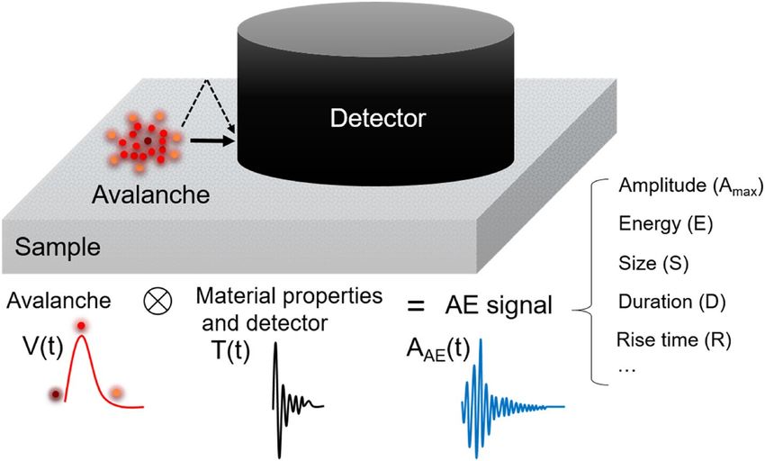
www.nature.com/scientificreports/
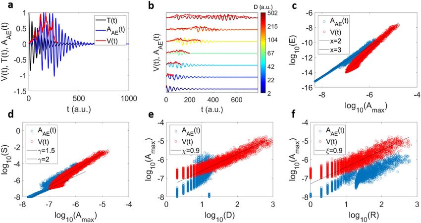
Figure 3. Scaling relations for the averaged source function before and after convolution. (a) Example of the
convolution (in blue) of an avalanche profile V(t) (in red) with a transfer function (cos (wt)e−qt with w=0.5
and q = 5 × 10⁻⁴ with time unit normalized to 1 (in black). (b) Examples of convoluted avalanche profiles for
different durations (blue to red when decreasing the b parameter) and the original profiles (in black). Both
convoluted and elementary profiles were normalized with respect to their maximum amplitudes. The scaling
γ
correlations E ∼ Axmax (c), S ∼ Amax (d), Amax ∼ Dχ(e) and Amax ∼ Rξ (f) for the original V(t) profiles (red
points) and after the convolution for AAE(t) (blue points).
function durations, the convoluted duration increases with the maximum amplitude of the source function and
changes the integrals to calculate EAE and SAE, which modify their scalings with respect to Amax. This behaviour
differs from the scaling of the rise time R which does not change with variable Amax after convolution (Fig. 3f).
In this toy model we hence observe both scenarios, x = 2 and x = 3, depending on the duration of the local strain
signal: if the source signal is short (e.g. delta function) the AE signal is identical or close to the transfer function
and we find x = 2. For long local events we find x = 3.
Model simulations with transfer functions
The collapse model. We now consider more realistic source functions and ask whether source functions
alone, without the interference of the transfer function, can generate the observed EAE ~ Amax2 scaling. For this
purpose, we construct a simple atomic model based on the mechanism leading to porous collapse. In this model
we choose random sites for the collapse and a feedback that stipulates that the next step depends on the collapsed
regions multiplied by a probability chosen from a probability distribution function f(t) as
Va (t) = f (t)Vs (t − 1). (13)
Here Vs(t − 1) is the is number of collapsed sites at t − 1 and f(t) is a Gaussian function centered at zero with
half width w. The product defines the number of attempted collapsing sites Va(t) that will be placed randomly in
space. The sites will successfully collapse if they do not overlap with previously collapsed sites. Thus, the avalanche
profile V(t) is defined by the collapsed sites per time Vs(t). The initial condition is the collapse of a single site
(Vs (t = 0) = 1) that is randomly chosen. When an avalanche ends because Vs(t − 1) = 0, the next avalanche is
chosen to start at a new random site with Vs(0) = 1 in an empty frame. The half width of f(t) is chosen as w = 1.4
in our simulations, more general conditions will be discussed in a forthcoming paper. This model is similar to
the mean field approximation of the non-equilibrium random field Ising model with power law distributed spin
flip avalanches at a critical width of the distribution of random fields60–63. Finite-size effects have an impact on
the cut-off of E, Amax, S etc. but not on the correlation between these quantities. This is caused by a direct impact
of the overlap between attempted sites Va(t) and previously collapsed sites Vs(t − 1). The widest scaling interval
is found when the overlap is reduced to zero. We hence use the Eq. (13) without placing actual sites in space and
accepting all sites to collapse successfully Va(t) = Vs(t) = V(t). Here we use avalanches profiles produced by the
equation V(t) = f(t)V(t − 1). Examples of the computed avalanche profiles are shown in Fig. 4 for different dura-
tions. The average avalanche p rofile11,37, generated by this model, is similar to the initially used average avalanche
profile (supplementary information section 5).
The PDFs are shown together with the maximum likelihood profiles of E, Amax and S in Fig. 4a,b. The PDFs
exhibit a good power law behavior with the exponents ε = 1.33 (for E), α = 1.66 (for Amax) and τ = 1.66 (for S).
The correlations between the avalanche magnitudes are given in Fig. 5 (red circles in c–f). The scaling between
E and Amax shows E ∼ A2max (Fig. 5c). The scaling between S and Amax follows the relation S ∼ Amax (Fig. 5d).
The duration of V(t), computed as the time when V(t) crosses a threshold, scales with Amax as shown in Fig. 5e.
The rise time scales in the same way as the duration (Fig. 5e,f). Our simple model exhibits the half-moon profile
of the correlation between the duration and the maximum amplitude.
Scientific Reports | (2021) 11:5590 | https://doi.org/10.1038/s41598-021-84688-7 5
Vol.:(0123456789)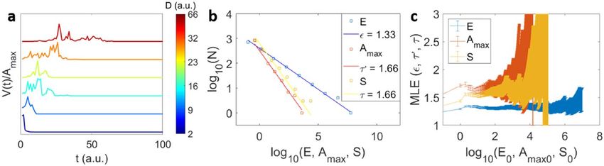
www.nature.com/scientificreports/
Figure 4. Avalanches of the collapse model. (a) Examples of normalized avalanche profiles V(t)/Amax with
different durations (blue to red means increasing the duration) for simulations of the model of Eq. (13). PDF (b)
and maximum likelihood exponent (MLE) (c) of the energy (E), maximum amplitude Amax and size S for the
model of Eq. (13).
Figure 5. Scaling relations of the collapse model before and after convolution. (a) Example of convolution
leading to AAE(t) with an avalanche profile V(t) (in red) and a transfer function T(t) = cos (wt)e−qt (in black).
(b) Examples of 6 convoluted avalanche profiles for different source functions V(t) with different durations, and
the same transfer function. Both convoluted and original profiles are normalized with respect to their maxima.
γ
(c–f) scaling relations E ∼ Axmax (c), S ∼ Amax (d), Amax ∼ Dχ(e) and Amax ∼ Rξ (f) for the original V(t)
profiles (red points) and after the convolution AAE(t) (blue points).
We now explore the scaling after convolution to AAE(t) with different transfer functions. As an example, we
consider again the transfer function T = cos (wt)e−qt , where w is the frequency and q a damping factor with
w = 1(1/t) and q = 10–7 (1/t2). Other transfer functions are shown in the Supplementary Material section 1, 3 and
4. The Fig. 5a shows an example of a single avalanche profile, the transfer function and the result of the convo-
lution. Different AE signals AAE(t) are shown in Fig. 5b for the same transfer function but different durations.
The scaling between E, Amax and S remains unperturbed by the convolution as shown in Fig. 5c,d. However, the
scaling between Amax and duration is different after convolution and strongly depends on the chosen transfer
function (see supplementary information section 2, 3 and 4) and the threshold that is used to define the duration
of AAE(t). The time evolution of AAE(t) is dominated by the decay of the transfer function. We now calculate the
rise time, defined as the time to reach Amax. The relation between the rise time R and the duration D is propor-
tional R ~ D for the V(t) profiles and it is preserved after the convolution, as shown in Fig. 5f and directly for the
convoluted profiles in Fig. 5b. The model is similar to spin-based models, such as the non-equilibrium random
odel37,60–63.
field Ising m
The slip model. We compare these results with mean field simulations of a simple slip model23. In contrast
to the collapse model, the slip model takes into account the long-range character of the elastic interactions
between weak spots in a slowly sheared solid. While the collapse model is more empirical in spirit, the mean
field model is a coarse-grained model that is based on the physical dynamics on scales as small as individual
weak spots in the material. It is again a threshold model, and the long-range interactions between the slips in
the material enable one to compute analytical solutions for the universal scaling behavior of the slip statistics.
Renormalization group methods have been used to show that this scaling behavior is the same as slips in slowly
deformed solids with slip localization, such as nanocrystals, bulk metallic glasses, rocks, jammed granular mate-
rials, friction and earthquakes23,25,60–63. The model assumes a solid that consists of N interacting cells, each of
Scientific Reports | (2021) 11:5590 | https://doi.org/10.1038/s41598-021-84688-7 6
Vol:.(1234567890)www.nature.com/scientificreports/
Figure 6. Scaling relations of the slip model before and after convolution. (a) Example of a convolution leading
to AAE(t) (in blue) from an avalanche profile V(t) (in red) and a transfer function T(t) = cos (wt)e−qt (in black).
(b) Examples of 6 convoluted avalanche profiles for different source functions V(t) with different durations, and
the same transfer function. Both convoluted and original profiles are normalized with respect to their maxima.
γ
(c–f) scaling relations E ∼ Axmax (c), S ∼ Amax (d), Amax ∼ Dχ(e) and Amax ∼ Rξ (f) for the original V(t)
profiles (red points) and after the convolution AAE(t) (blue points). For e) and f) the exact exponent values in
mean field theory are Χ=1 and ξ=1.
which can slip by a random amount when the local stress reaches a local stress threshold. When a cell slips the
released stress is equally redistributed to the other cells, which can trigger other cells to slip also in a slip ava-
lanche. A slip avalanche ends when the stress at all cells is below the local failure stress. Then the external loading
stress is slowly increased until the next cell slips, triggering the next avalanche. In its simplest version the model
predicts power law distributed avalanche sizes, and durations. The time profiles of the avalanche propagation
speeds (averaged over all avalanches of the same size or duration) follow simple scaling functions that can be
computed analytically23. Many predictions for the scaling properties of the model are given in23,25,60–63. There
are related spin flip models, such as the non-equilibrium random field Ising model, which give similar scaling
results60–62, and they are likely even more closely related to the model introduced here because of their notable
disorder dependence. Here, the source time functions are extracted from the slip model and convolved with the
transfer function T(t). The results are shown in the Fig. 6.
Following the same steps as previously, we plot the transfer function T(t) with an example of a source func-
tion V(t) and the correspondent convolution AAE(t) in Fig. 6a. Figure 6b shows some examples of V(t) and the
corresponding AAE(t) for increasing durations. The correlation E ∼ Axmax exhibits x = 3 for the local strain signal
γ
V(t) and x = 2 for the measured AE signal AAE(t) (Fig. 6c). Similarly, the scaling relation S ∼ Amax shows γ = 2
for V(t) and γ = 1.5 for AAE(t). This change2of the scaling relation exponent is expected as shown previously for
the average source function V(t) = ate−bt (see Fig. 3). The duration scaling with Amax before the convolution
is clearly different for the collapse model and the slip model, after convolution the initial scaling is almost lost.
Only the rise time R preserves qualitatively the scaling after convolution (Fig. 6f).
Conclusion
We have shown that the measured AE spectrum, i.e. the macroscopic jerk spectrum of a sample, does not reflect
the initial avalanche distribution V(t) nor the predictions of mean field theory. There are two main reasons.
Firstly, the measured AE is modified by the transfer function in a well-defined fashion. This modification is most
notorious if the time and frequency scales of the initial avalanche formation (some microseconds in many cases)
differs greatly from the inverse frequency of the sample ringing and hence the transfer function. Ringing times
are typically between several microseconds and some milliseconds. This time scale depends on the sample size
(decreasing transfer time with decreasing sample size) and the nature of the initial avalanche. Crack propagation
and dislocation dynamics are fairly similar in their local duration D while ferroelectric and ferroelastic domain
movements are often much slower. Nevertheless, the general rule is that the transfer function shifts exponents
to x = 2 while x = 3 has never been observed experimentally.
Scientific Reports | (2021) 11:5590 | https://doi.org/10.1038/s41598-021-84688-7 7
Vol.:(0123456789)www.nature.com/scientificreports/
Comparing the toy model with the more realistic profiles of the transfer function highlights the reasons. The
average profile of the toy model is very broad. In contrast, the simulated avalanche profiles and experimental
profiles show few very sharp peaks, often only one dominant peak. The convolution with the transfer function
then yields the transfer function as AAE. All information about the initial duration of the source event and its
line profiles is lost and only the transfer function is measured. This seems to be the fate of most AE spectra so
that a detailed analysis of the observed jerk profiles only reveals information about the transfer function and says
little about the local avalanche mechanism. The main information is hence the parameter x: x = 2 means that the
local process is fast compared with the sample ringing, x > 2 means that some information about the local time
scale could be obtained from AE spectra.
The observation x = 2 does not mean that the avalanche process does not follow the predicted mean field
scaling. The observed duration is usually not the correct time scale because it is strongly modified by the transfer
function. If the spectrum V(t) contains narrow peaks, then the integral is determined by the integral over the
peak area and not by the much wider integration interval over the duration of the avalanche. This effect is very
common in ferroelastics where a domain collapses or scatters with another domain. After one massive event,
there are long-term relaxations, which contribute to the duration D but contain very little energy. In this case
we find that x = 2.
The third fundamentally important result is that the duration is in all cases a very complex quantity, which
cannot be approximated easily. In contrast, we find that the rise time R represents the avalanche formation and
propagation much better (supplementary information section 7). It is close to the local rise time and is less pol-
luted by the effect of the transfer function.
Different models for avalanches statistics yield similar macroscopic behaviour while some characteristic dif-
ferences occur23,24. The power law distributions for energy and sizes are invariant (supplementary information
section 5), however. The main differences stem from the role played by the duration. The ‘half-moon’ shape of
Amax(D) and Amax(R) is well reproduced in the collapse model but much less in the slip model. This result points
to the usefulness of the duration and specially rise time as AE avalanche characteristics, which allow at least a
partial distinction between different atomic avalanche mechanisms. Further work on the distinction between
avalanches models and their consequences for AE measurements are planned.
Data availability
The data that support the findings of this study are available from the corresponding author upon reasonable
request.
Received: 24 November 2020; Accepted: 17 February 2021
References
1. Davidsen, J., Stanchits, S. & Dresen, G. Scaling and universality in rock fracture. Phys. Rev. Lett. https://doi.org/10.1103/PhysR
evLett.98.125502 (2007).
2. Salje, E. K. H. et al. Failure mechanism in porous materials under compression: crackling noise in mesoporous SiO2. Philos. Mag.
Lett. https://doi.org/10.1080/09500839.2011.596491 (2011).
3. de Arcangelis, L. & Redner, S. A random fuse model for breaking processes. J. Phys. Lett. https://doi.org/10.1051/jphyslet:01985
0046013058500 (1985).
4. Zapperi, S., Ray, P., Stanley, H. E. & Vespignani, A. First-order transition in the breakdown of disordered media. Phys. Rev. Lett.
https://doi.org/10.1103/PhysRevLett.78.1408 (1997).
5. Moreno, Y., Gómez, J. B. & Pacheco, A. F. Fracture and second-order phase transitions. Phys. Rev. Lett. https://doi.org/10.1103/
PhysRevLett.85.2865 (2000).
6. Alava, M. J., Nukala, P. K. V. V. & Zapperi, S. Statistical models of fracture. Adv. Phys. https://doi.org/10.1080/000187303007415
18 (2006).
7. Davidsen, J. et al. Triggering processes in rock fracture. Phys. Rev. Lett. https://doi.org/10.1103/PhysRevLett.119.068501 (2017).
8. Friedman, N. et al. Statistics of dislocation slip avalanches in nanosized single crystals show tuned critical behavior predicted by
a simple mean field model. Phys. Rev. Lett. 109, 095507 (2012).
9. Maaß, R., Wraith, M., Uhl, J. T., Greer, J. R. & Dahmen, K. A. Slip statistics of dislocation avalanches under different loading modes.
Phys. Rev. E Stat. Nonlinear Soft Matter Phys. https://doi.org/10.1103/PhysRevE.91.042403 (2015).
10. Antonaglia, J. et al. Tuned critical avalanche scaling in bulk metallic glasses. Sci. Rep. https://doi.org/10.1038/srep04382 (2014).
11. Denisov, D. V. et al. Universal slip dynamics in metallic glasses and granular matter—linking frictional weakening with inertial
effects. Sci. Rep. https://doi.org/10.1038/srep43376 (2017).
12. Rosti, J., Koivisto, J. & Alava, M. J. Statistics of acoustic emission in paper fracture: precursors and criticality. J. Stat. Mech. Theory
Exp. https://doi.org/10.1088/1742-5468/2010/02/P02016 (2010).
13. Baró, J. et al. Statistical similarity between the compression of a porous material and earthquakes. Phys. Rev. Lett. https://doi.
org/10.1103/PhysRevLett.110.088702 (2013).
14. Salje, E. K. H. & Dahmen, K. A. Crackling noise in disordered materials. Annu. Rev. Condens. Matter Phys. 5, 233–254 (2014).
15. Wright, W. J. et al. Experimental evidence for both progressive and simultaneous shear during quasistatic compression of a bulk
metallic glass. J. Appl. Phys. https://doi.org/10.1063/1.4942004 (2016).
16. Chen, Y., Wang, Q., Ding, X., Sun, J. & Salje, E. K. H. Avalanches and mixing behavior of porous 316L stainless steel under tension.
Appl. Phys. Lett. https://doi.org/10.1063/1.5144069 (2020).
17. Chen, Y., Ding, X., Fang, D., Sun, J. & Salje, E. K. H. Acoustic emission from porous collapse and moving dislocations in granular
Mg-Ho alloys under compression and tension. Sci. Rep. https://doi.org/10.1038/s41598-018-37604-5 (2019).
18. Salje, E. K. H., Wang, X., Ding, X. & Scott, J. F. Ultrafast switching in avalanche-driven ferroelectrics by supersonic kink move-
ments. Adv. Funct. Mater. https://doi.org/10.1002/adfm.201700367 (2017).
19. Nataf, G. F. et al. Avalanches in compressed porous SiO2-based materials. Phys. Rev. E Stat. Nonlinear Soft Matter Phys. https://
doi.org/10.1103/PhysRevE.90.022405 (2014).
20. Nataf, G. F. et al. Predicting failure: acoustic emission of berlinite under compression. J. Phys. Condens. Matter https://doi.
org/10.1088/0953-8984/26/27/275401 (2014).
Scientific Reports | (2021) 11:5590 | https://doi.org/10.1038/s41598-021-84688-7 8
Vol:.(1234567890)www.nature.com/scientificreports/
21. Castillo-Villa, P. O. et al. Crackling noise during failure of alumina under compression: the effect of porosity. J. Phys. Condens.
Matter https://doi.org/10.1088/0953-8984/25/29/292202 (2013).
22. Salje, E. K. H. et al. Noise of collapsing minerals: predictability of the compressional failure in goethite mines. Am. Miner. https://
doi.org/10.2138/am.2013.4319 (2013).
23. Dahmen, K. A., Ben-Zion, Y. & Uhl, J. T. A simple analytic theory for the statistics of avalanches in sheared granular materials.
Nat. Phys. https://doi.org/10.1038/nphys1957 (2011).
24. Hidalgo, R. C., Grosse, C. U., Kun, F., Reinhardt, H. W. & Herrmann, H. J. Evolution of percolating force chains in compressed
granular media. Phys. Rev. Lett. https://doi.org/10.1103/PhysRevLett.89.205501 (2002).
25. Sornette, D. Mean-field solution of a block-spring model of earthquakes. J. Phys. I https://doi.org/10.1051/jp1:1992269 (1992).
26. Kadanoff, L. P., Nagel, S. R., Wu, L. & Zhou, S. M. Scaling and universality in avalanches. Phys. Rev. A https://doi.org/10.1103/
PhysRevA.39.6524 (1989).
27. Bak, P., Tang, C. & Wiesenfeld, K. Self-organized criticality: an explanation of the 1/f noise. Phys. Rev. Lett. https: //doi.org/10.1103/
PhysRevLett.59.381 (1987).
28. He, X., Ding, X., Sun, J. & Salje, E. K. H. Parabolic temporal profiles of non-spanning avalanches and their importance for ferroic
switching. Appl. Phys. Lett. https://doi.org/10.1063/1.4942387 (2016).
29. Jiang, X., Liu, H., Main, I. G. & Salje, E. K. H. Predicting mining collapse: superjerks and the appearance of record-breaking events
in coal as collapse precursors. Phys. Rev. E https://doi.org/10.1103/PhysRevE.96.023004 (2017).
30. Salje, E. K. H., Xue, D., Ding, X., Dahmen, K. A. & Scott, J. F. Ferroelectric switching and scale invariant avalanches in BaTiO3.
Phys. Rev. Lett. 014415, 1–8 (2019).
31. Zapperi, S., Cizeau, P. & Durin, G. Dynamics of a ferromagnetic domain wall: avalanches, depinning transition, and the Barkhausen
effect. Phys. Rev. B Condens. Matter Mater. Phys. https://doi.org/10.1103/PhysRevB.58.6353 (1998).
32. Scruby, C. B. An introduction to acoustic emission. J. Phys. E. https://doi.org/10.1088/0022-3735/20/8/001 (1987).
33. Lu, G., Li, S., Ding, X., Sun, J. & Salje, E. K. H. Ferroelectric switching in ferroelastic materials with rough surfaces. Sci. Rep. https
://doi.org/10.1038/s41598-019-52240-3 (2019).
34. Dul’Kin, E., Salje, E. K. H., Aktas, O., Whatmore, R. W. & Roth, M. Ferroelectric precursor behavior of highly cation-ordered
PbSc0.5Ta0.5O3 detected by acoustic emission: tweed and polar nanoregions. Appl. Phys. Lett. https://doi.org/10.1063/1.4902511
(2014).
35. Lu, G., Li, S., Ding, X., Sun, J. & Salje, E. K. H. Electrically driven ferroelastic domain walls, domain wall interactions, and moving
needle domains. Phys. Rev. Mater. https://doi.org/10.1103/PhysRevMaterials.3.114405 (2019).
36. Salje, E. K. H., Wang, X., Ding, X. & Sun, J. Simulating acoustic emission: the noise of collapsing domains. Phys. Rev. B Condens.
Matter Mater. Phys. https://doi.org/10.1103/PhysRevB.90.064103 (2014).
37. McFaul, L. W., Wright, W. J., Sickle, J. & Dahmen, K. A. Force oscillations distort avalanche shapes. Mater. Res. Lett. 7, 496–502
(2019).
38. Stojanova, M., Santucci, S., Vanel, L. & Ramos, O. High frequency monitoring reveals aftershocks in subcritical crack growth. Phys.
Rev. Lett. https://doi.org/10.1103/PhysRevLett.112.115502 (2014).
39. Ishibashi, Y. & Iwata, M. Activation energy of ferroelectric domain wall. J. Phys. Soc. Jpn. 89, 014705 (2020).
40. Orihara, H., Hashimoto, S. & Ishibashi, Y. A theory of D-E hysteresis loop based on the Avrami model. J. Phys. Soc. Jpn. 63,
1031–1035 (1994).
41. Salje, E. K. H. et al. (eds) Avalanches in Functional Materials and Geophysics (Springer, Berlin, 2017). https://doi.org/10.1007/978-
3-319-45612-6.
42. Weiss, J. Ice: the paradigm of wild plasticity. Philos. Trans. R. Soc. A Math. Phys. Eng. Sci. 377, 20180260 (2019).
43. Vu, C.-C., Amitrano, D., Plé, O. & Weiss, J. Compressive failure as a critical transition: experimental evidence and mapping onto
the universality class of depinning. Phys. Rev. Lett. 122, 015502 (2019).
44. Baró, J. et al. Experimental evidence of accelerated seismic release without critical failure in acoustic emissions of compressed
nanoporous materials. Phys. Rev. Lett. 120, 245501 (2018).
45. Vu, C. C. & Weiss, J. Asymmetric damage avalanche shape in quasibrittle materials and subavalanche (aftershock) clusters. Phys.
Rev. Lett. 125, 105502 (2020).
46. Forbes, M., Letcher, S. & Stepanishen, P. A wave vector, time-domain method of forward projecting time-dependent pressure
fields. J. Acoust. Soc. Am. 90, 2782–2793 (1991).
47. Planès, T. & Larose, E. A review of ultrasonic Coda Wave Interferometry in concrete. Cem. Concr. Res. 53, 248–255 (2013).
48. Vu, C. C., Weiss, J., Plé, O., Amitrano, D. & Vandembroucq, D. Revisiting statistical size effects on compressive failure of hetero-
geneous materials, with a special focus on concrete. J. Mech. Phys. Solids 121, 47–70 (2018).
49. Salje, E. K. H., Aktas, O., Carpenter, M. A., Laguta, V. V. & Scott, J. F. Domains within domains and walls within walls: evidence
for polar domains in cryogenic SrTiO3. Phys. Rev. Lett. 111, 247603 (2013).
50. Aktas, O., Crossley, S., Carpenter, M. A. & Salje, E. K. H. Polar correlations and defect-induced ferroelectricity in cryogenic KTaO3.
Phys. Rev. B Condens. Matter Mater. Phys. 90, 165309 (2014).
51. Salje, E. K. H., Zhao, Z., Ding, X. & Sun, J. Mechanical spectroscopy in twinned minerals: simulation of resonance patterns at high
frequencies. Am. Miner. 98, 1449–1458 (2013).
52. Salje, E. K. H. et al. Elastic excitations in BaTiO3 single crystals and ceramics: mobile domain boundaries and polar nanoregions
observed by resonant ultrasonic spectroscopy. Phys. Rev. B Condens. Matter Mater. Phys. 87, 014106 (2013).
53. Safarik, D. J., Salje, E. K. H. & Lashley, J. C. Spectral analysis of resonance ultrasonic spectroscopy: Kramers–Kronig analysis, Fano
profiles, and the case of precursor softening in SnTe:Cr. Appl. Phys. Lett. 97, 111907 (2010).
54. Carpenter, M. A., Salje, E. K. H. & Howard, C. J. Magnetoelastic coupling and multiferroic ferroelastic/magnetic phase transitions
in the perovskite KMnF3. Phys. Rev. B Condens. Matter Mater. Phys. 85, 224430 (2012).
55. Salje, E. K. H. et al. Tin telluride: a weakly co-elastic metal. Phys. Rev. B Condens. Matter Mater. Phys. 82, 184112 (2010).
56. Dobrinevski, A., Le Doussal, P. & Wiese, K. J. Statistics of avalanches with relaxation and Barkhausen noise: a solvable model. Phys.
Rev. E Stat. Nonlinear Soft Matter Phys. 88, 032106 (2013).
57. Rosti, J. et al. Line creep in paper peeling. Int. J. Fract. 151, 281–297 (2008).
58. Berndt, C. C. Failure processes within ceramic coatings at high temperatures. J. Mater. Sci. 24, 3511–3520 (1989).
59. Wang, D., Wang, Z., Li, P., Chen, Y. & Li, H. Dual Gaussian attenuation model of ultrasonic echo and its parameter estimation.
AIP Adv. 9, 055213 (2019).
60. Sethna, J. P., Dahmen, K. A. & Myers, C. R. Crackling noise. Nature 410, 242–250 (2001).
61. Dahmen, K. & Sethna, J. P. Hysteresis, avalanches, and disorder-induced critical scaling: a renormalization-group approach. Phys.
Rev. B Condens. Matter Mater. Phys. 53, 14872–14905 (1996).
62. Sethna, J. P. et al. Hysteresis and hierarchies: dynamics of disorder-driven first-order phase transformations. Phys. Rev. Lett. 70,
3347–3350 (1993).
63. Leblanc, M., Angheluta, L., Dahmen, K. & Goldenfeld, N. Universal fluctuations and extreme statistics of avalanches near the
depinning transition. Phys. Rev. E Stat. Nonlinear Soft Matter Phys. 87, 022126 (2013).
Scientific Reports | (2021) 11:5590 | https://doi.org/10.1038/s41598-021-84688-7 9
Vol.:(0123456789)www.nature.com/scientificreports/
Acknowledgements
This research was supported by a Grant from EPSRC (No. EP/P024904/1) to E.K.H.S. and B.C. This project has
received funding from the EU’s Horizon 2020 programme under the Marie Skłodowska-Curie Grant Agreement
No. 861153.
Author contributions
E.K.H.S., B.C., and K.A.D. wrote the main manuscript text. B.C. and B.G. developed the analysis of the avalanches
models. K.A. and S.R. developed the SLIP avalanche model. All authors reviewed the manuscript.
Competing interests
The authors declare no competing interests.
Additional information
Supplementary Information The online version contains supplementary material available at https://doi.
org/10.1038/s41598-021-84688-7.
Correspondence and requests for materials should be addressed to B.C.
Reprints and permissions information is available at www.nature.com/reprints.
Publisher’s note Springer Nature remains neutral with regard to jurisdictional claims in published maps and
institutional affiliations.
Open Access This article is licensed under a Creative Commons Attribution 4.0 International
License, which permits use, sharing, adaptation, distribution and reproduction in any medium or
format, as long as you give appropriate credit to the original author(s) and the source, provide a link to the
Creative Commons licence, and indicate if changes were made. The images or other third party material in this
article are included in the article’s Creative Commons licence, unless indicated otherwise in a credit line to the
material. If material is not included in the article’s Creative Commons licence and your intended use is not
permitted by statutory regulation or exceeds the permitted use, you will need to obtain permission directly from
the copyright holder. To view a copy of this licence, visit http://creativecommons.org/licenses/by/4.0/.
© The Author(s) 2021
Scientific Reports | (2021) 11:5590 | https://doi.org/10.1038/s41598-021-84688-7 10
Vol:.(1234567890)You can also read