Fast analytical calculation of the random pair counts for realistic survey geometry
←
→
Page content transcription
If your browser does not render page correctly, please read the page content below
A&A 646, A40 (2021)
https://doi.org/10.1051/0004-6361/202039603                                                                                                             Astronomy
c M.-A. Breton and S. de la Torre 2021                                                                                                                   &
                                                                                                                                                        Astrophysics

  Fast analytical calculation of the random pair counts for realistic
                           survey geometry
                                                     Michel-Andrès Breton and Sylvain de la Torre

     Aix Marseille Univ., CNRS, CNES, LAM, Marseille, France
     e-mail: michel-andres.breton@lam.fr
     Received 6 October 2020 / Accepted 14 December 2020

                                                                                   ABSTRACT

     Galaxy clustering is a standard cosmological probe that is commonly analysed through two-point statistics. In observations, the es-
     timation of the two-point correlation function crucially relies on counting pairs in a random catalogue. The latter contains a large
     number of randomly distributed points, which accounts for the survey window function. Random pair counts can also be advanta-
     geously used for modelling the window function in the observed power spectrum. Since pair counting scales as O(N 2 ), where N is
     the number of points, the computational time to measure random pair counts can be very expensive for large surveys. In this work,
     we present an alternative approach for estimating those counts that does not rely on the use of a random catalogue. We derived an
     analytical expression for the anisotropic random-random pair counts that accounts for the galaxy radial distance distribution, survey
     geometry, and possible galaxy weights. We show that a prerequisite is the estimation of the two-point correlation function of the
     angular selection function, which can be obtained efficiently using pixelated angular maps. Considering the cases of the VIPERS and
     SDSS-BOSS redshift surveys, we find that the analytical calculation is in excellent agreement with the pair counts obtained from
     random catalogues. The main advantage of this approach is that the primary calculation only takes a few minutes on a single CPU
     and it does not depend on the number of random points. Furthermore, it allows for an accuracy on the monopole equivalent to what
     we would otherwise obtain when using a random catalogue with about 1500 times more points than in the data at hand. We also
     describe and test an approximate expression for data-random pair counts that is less accurate than for random-random counts, but still
     provides subpercent accuracy on the monopole. The presented formalism should be very useful in accounting for the window function
     in next-generation surveys, which will necessitate accurate two-point window function estimates over huge observed cosmological
     volumes.
     Key words. cosmology: miscellaneous – large-scale structure of Universe – methods: numerical – methods: statistical

1. Introduction                                                                                anisotropy makes observed galaxy n-point statistics sensitive to
                                                                                               the strength of gravity acting on the large-scale structure (Kaiser
The spatial distribution of galaxies has a long history of pro-
                                                                                               1987; Guzzo et al. 2008).
viding cosmological parameter constraints (e.g., Strauss et al.
                                                                                                    Formally, the two-point correlation function is the excess
1992; Vogeley et al. 1992; Maddox et al. 1996; Peacock et al.
                                                                                               probability of finding a pair of objects at a given distance,
2001; Cole et al. 2005; Tegmark et al. 2006; Percival et al. 2010;
                                                                                               with respect to the expectation in a random Poisson distribu-
Blake et al. 2012; de la Torre et al. 2013; Alam et al. 2017;
                                                                                               tion of points. In practice, we rely on statistical estimators to
eBOSS Collaboration 2020, and references therein). This arises
                                                                                               measure the correlation function from galaxy survey data. The
from the fact that the statistical properties of galaxies, partic-
                                                                                               first estimator was proposed by Peebles & Hauser (1974), tak-
ularly spatial ones, can be predicted by cosmological models.
                                                                                               ing the form ξPH (s) = DD(s)/RR(s) − 1, where DD and RR
When analysing galaxy clustering, we usually compress the
                                                                                               are the normalised number of distinct pairs separated by a vec-
information by using summary statistics, the most natural one
                                                                                               tor s, in the data and random samples, respectively. The lat-
being the two-point correlation function or its Fourier counter-
                                                                                               ter sample is constructed such that random points follow the
part in the power spectrum. This is due to the nearly Gaussian
                                                                                               same radial and angular selection functions as the data. Other
nature of primordial matter perturbations, which are almost fully
                                                                                               estimators were later proposed (Hewett 1982; Davis & Peebles
described by their two-point statistics. Although gravitational
                                                                                               1983; Hamilton 1993) to reduce the estimation variance, notably
evolution leads to non-Gaussianity, and in turn, non-vanishing
                                                                                               induced by discreteness and boundary effects. In particular,
higher-order n-point statistics, two-point statistics continues to
                                                                                               the Landy & Szalay (1993) minimum-variance estimator was
be very informative.
                                                                                               designed such that for any survey geometry, its variance is nearly
     Despite the cosmological principle that implies that the cor-
                                                                                               Poissonian. This estimator, defined as
relation function is isotropic, meaning that it is only a function
of the norm of the separation vector, because of the way the                                                 DD(s) − 2DR(s) + RR(s)
line-of-sight distance is measured in redshift surveys and the                                 ξLS (s) =                            ,                                                   (1)
                                                                                                                     RR(s)
presence of peculiar velocities, the observed correlation func-
tion becomes anisotropic. These velocities are induced on large                                makes use of additional data-random pairs DR. To estimate
scales by the coherent convergence of matter towards overden-                                  the correlation function, we therefore need to compute the
sities as part of the general process of structure growth. This                                number of pairs as a function of the separation. To avoid
                                                                                                                                                                           A40, page 1 of 10

              Open Access article, published by EDP Sciences, under the terms of the Creative Commons Attribution License (https://creativecommons.org/licenses/by/4.0),
                               which permits unrestricted use, distribution, and reproduction in any medium, provided the original work is properly cited.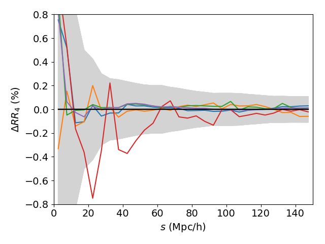
A&A 646, A40 (2021)
introducing bias in the estimator and to minimise variance, practice, as in the case of fibre or slit collision, for instance, we
the random catalogue must be much larger than the data cata- can assume independence in building RR but while applying an
logue (Landy & Szalay 1993; Keihänen et al. 2019). We usually object or pairwise weighting scheme to account for those cor-
consider that taking at least about 20−50 times more random relations (e.g., de la Torre et al. 2013; Bianchi & Percival 2017;
points than objects in the data is enough to avoid introducing Ross et al. 2017).
additional variance (e.g., Samushia et al. 2012; de la Torre et al. In this paper, we provide general expressions for the
2013; Sánchez et al. 2017; Bautista et al. 2021). A problem is anisotropic RR and DR pair counts in the case of a realis-
that the computational time for direct pair counting scales as tic survey geometry, including the cases for the different def-
O(N 2 ), with N the number of elements in a given sample. initions of the pair’s line of sight. We apply this formalism
Nonetheless, the complexity can be reduced, at best, to O(N) to the VIMOS Public Extragalactic Redshift Survey (VIPERS,
using appropriate algorithms and various efficient codes that Guzzo et al. 2014; Garilli et al. 2014) and Sloan Digital Sky
implement them have been developed (e.g., Moore et al. 2001; Survey Baryon Oscillation Spectroscopic Survey (SDSS-BOSS,
Jarvis et al. 2004; Alonso 2012; Hearin et al. 2017; Marulli et al. Eisenstein et al. 2011; Dawson et al. 2013) and we perform an
2016; Slepian & Eisenstein 2016; Sinha & Garrison 2020). For assessment of the accuracy of the method.
the random-random pairs calculation specifically, additional This paper is organised as follows. Section 2 presents the for-
strategies can be used to speed up the computation beyond par- malism for random-random and data-random pair counts. This
allelisation, such as splitting the random sample and averag- formalism is applied and its accuracy assessed in Sect. 3. We
ing the counts over subsamples (Keihänen et al. 2019). Still, for conclude in Sect. 4.
large surveys, the computational time for estimating the corre-
lation function, especially random-random pairs, can become
an issue. In particular, next-generation surveys such as Euclid 2. Formalism
(Laureijs et al. 2011) or DESI (DESI Collaboration 2016), will In this section, we provide the analytical formalism for the
necessitate random samples as large as about 3 × 10⁸ objects in random-random and data-random pair counts.
several redshift bins, or even larger if we consider a single, wide-
redshift bin (e.g., Mueller et al. 2019; Castorina et al. 2019).
The role of random-random pair counts in the correlation 2.1. Random-random pairs
function estimator is to account for the survey selection func-
tion, that is, the effective observed volume and its impact on In a survey sample where sources are selected in redshift, the
the data-data pair counts. In Fourier space instead, common number of sources in a given radial distance interval [rmin , rmax ]
estimators for the power spectrum (e.g., Feldman et al. 1994; is:
Yamamoto et al. 2006) provide a direct estimate of the window- Z rmax
convolved power spectrum. To be able to compare theoretical N(rmin , rmax ) = p(r)dr, (3)
predictions to observations, it is necessary to convolve the model rmin
power spectrum with the survey window function. This convo-
lution is computationally expensive in the likelihood analysis, with p(r) the number of sources as function of the radial distance
but it can be done efficiently by performing a multiplication in r and
configuration space, as proposed by Wilson et al. (2017). The Z π Z 2π
latter shows that the window-convolved power spectrum multi- p(r) = r n(r)
2
sin(θ) W(θ, ϕ)dθdϕ, (4)
poles moments P̂` (k) can be written as: 0 0
X q 2` + 1 RR ` (s) where W(θ, ϕ) is the survey angular selection function in spher-
P̂` (k) = H A`p ξ` (s)N , (2)
p,q
2q + 1 2πs2 ∆s ical coordinates. The latter encodes the probability of observing
a source at any angular position on the sky and takes values from
where H denotes the Hankel transform, Aq`p are coefficients, 0 to 1. Here, n(r) is the source number density given by
ξ` (s) are model correlation function multipole moments, N is
0 for r < rmin ,
a normalisation factor, RR` (s) are the multipole moments of
p(r)
n(r) = rmin < r < rmax ,
the random-random pair counts, and ∆s is the bin size in s 2 for (5)
(Wilson et al. 2017; Beutler et al. 2017). 04πr hWi
for r > rmax ,
Random-random pairs counts are a purely geometrical quan-
tity that depends on cosmology only through the radial selection with hWi the angular selection function averaged over the full
function, which is defined in terms of the radial comoving dis- sky. We note that radial weights, such as those of Feldman et al.
tance. In the case of a simple geometry, such as a cubical vol- (1994), can be included straightforwardly in the p(r), such that
ume with constant number density and periodic boundary con- this becomes a weighted radial distribution in the equations. The
ditions, the RR pair counts can be predicted from the appropri- total number of observed sources is therefore:
ately normalised ratio between the spherical shell volume at s Z rmax Z π Z 2π
and the total volume. In the case of a realistic survey geometry,
and taking advantage of the fact that radial and angular selection N(rmin , rmax ) = 2
r n(r) sin(θ) W(θ, ϕ)dϕdθdr. (6)
rmin 0 0
functions are usually assumed to be uncorrelated, Demina et al.
(2018) developed a semi-analytical method to compute the RR In RR(s), we correlate points at two different positions r1 and r2
and DR pair counts along the directions parallel and trans- and it is convenient to write
verse to the line of sight, but still using a random sample to
account for angular correlations. In fact, the process of spectro- s
!2
scopic observation can break this assumption, making radial and s s
r2 (r1 , s, µ) = r1 1 + 2µ + , (7)
angular selection functions partially correlated. Nonetheless, in r1 r1
A40, page 2 of 10
M.-A. Breton and S. de la Torre: Fast RR and DR calculation
with s = r2 − r1 and µ = r1 · s/r1 s. RR is obtained by integrating with r(r1 , s, µ) = r1 1 + µs/r + s2 /(2r)2 . Finally, we note that
p
the angular and radial selection functions first over (r1 , θ, ϕ) and in order to cross-correlate tracers with different radial selection
then over the volume defined by the separation (s, θ̃, ϕ̃) as: functions but the same angular selection function, we can use the
Z rmax Z smax Z π Z π same formalism but with different nA (r1 ) and nB (r2 ) in Eqs. (12)–
RR(smin , smax ) = r12 n(r1 ) s2 sin θ sin θ̃ (14).
rmin smin 0 0
Z 2π Z 2π
× n(r2 )W(θ1 , ϕ1 ) 2.2. Data-random pairs
0 0
The Landy & Szalay (1993) estimator includes data-random
× W(θ2 , ϕ2 )dr1 dsdθdθ̃dϕdϕ̃, (8) pairs to minimise variance. A similar formalism to that used for
where θ1 , ϕ1 (θ2 , ϕ2 ) are the angular positions at r1 (r2 ). Let us random-random pair counts can be employed to evaluate data-
define r̂1 = r1 /r1 and r̂2 = r2 /r2 , we have then random pair counts. However, contrarily to the RR case, we now
Z Z have to cross-correlate a discrete set of sources with a continuous
d r̂1 W(r̂1 )W(r̂2 ) =
2
d2 r̂1 W(r̂1 )W(r̂1 + φ), (9) random distribution. The discrete limit of Eq. (3) is
4π 4π
N Z rmax Z
X
and the correlation function of the angular selection function is N(rmin , rmax ) = δD (r − ri )drd2 r̂, (16)
Z i=0 rmin 4π
1
ω(φ) = hW(r̂1 )W(r̂1 + φ)i = d2 r̂1 W(r̂1 )W(r̂1 + φ). (10)
4π 4π with δD the Dirac delta function, r = (r, θ, ϕ), and ri the ith
source position in the data vector. We can then use the same
In our case, since we auto-correlate randoms points, RR will only
methodology as in Sect. 2.1. To make the computation of the
depend on the angular separation (for cross-correlations with dif-
data-random pair counts tractable we make the assumption:
ferent angular selection functions, we would need to keep the
angular dependence). This means that we can write ω(φ) = ω(φ), N Z rmax Z N N
X 1 XX
where we have dr1 d2 r̂1 δD (r1 − ri )W(r̂1 + φ) ≈
i=0 rmin 4π N i=0 j=0
r1 + r22 − s2
2
φ(r1 , r2 , s) = arccos · (11) Z rmax Z
2r1 r2 dr1 δD (r1 − ri ) d2 r̂1 δD (r̂1 − r̂ j )W(r̂1 + φ), (17)
rmin 4π
We note that in the absence of an angular mask, that is, when we
evenly probe the full sky, ω(φ) = 1. In compiling these results, with r̂1 = (θ, ϕ) and r̂i the angular position in the data vector.
we find that: Under this assumption, the angular correlation at a particular
Z rmax point is given by that of the whole sample. For a large-enough
RR(smin , smax , µmin , µmax ) = 8π2
r12 n(r1 ) N and a sufficiently homogeneous angular sampling of the data,
rmin the approximation should hold. We find that:
Z smax Z µ∗max
× s2 n(r2 )ω(φ)dr1 dsdµ. (12) XN
4π rmax
Z
smin µ∗min DR(smin , smax , µmin , µmax ) = δD (r1 − ri )
i=0
N rmin
We note that we have implicitly assumed an ‘end-point’ defini- Z smax Z µ∗max
tion for the pair line of sight, that is, for every separation, the × s2 n(r2 )
direction of the line of sight coincides with that of r1 . With this smin µ∗min
definition, we can just use (µ∗min , µ∗max ) = (µmin , µmax ) for the inte- Z 2π
gral limits in Eq. (12). In the case of the ‘mid-point’ definition × ωDR (φ)dr1 dsdµdϕ, (18)
for the pair line of sight, where µ = r · s/rs with r = 21 (r1 + r2 ), 0
we can use the same equation, but we need to change the integral with
limits for each {r1 , s, µ} as:
N Z
q 1 X
−s + sµ2 + µ s2 µ2 − s2 + 4r12 ωDR (φ) = d2 r̂1 δD (r̂1 − r̂ j )W(r̂1 + φ), (19)
4π j=0
µ∗ (r1 , s, µ) = · (13) 4π
2r1
where we integrate over all the data and angular selection
We note that for the end-point definition it is important to com- function positions. In practice, we can cross-correlate a map
pute pairs with µ < 0 since the correlation function in that case
containing the galaxy number density per pixel with the angu-
is not symmetric by pair exchange. For applications involving
lar selection function map. Introducing a generic data weight wi ,
random-random multipole moments directly, the latter can be
for each source and assuming that the angular cross-correlation
defined as:
function does not depend on the pair orientation, we obtain
2 (2` + 1)
Z rmax
RR` (smin , smax ) = 8π r12 n(r1 ) N Z
2 8π2 X rmax
rmin DR(smin , smax , µmin , µmax ) = δD (r1 − ri )wi
Z smax Z 1 N i=0 rmin
× s2 n(r2 )ω(φ)L` (µ† )dr1 dsdµ, (14) Z smax Z µ∗max
smin −1
× s2 n(r2 )ωDR (φ)dr1 dsdµ. (20)
µ∗min
with L` the Legendre polynomial of order `. For the end-point smin
definition, µ† = µ, while for the mid-point definition we have We can already see that the calculation involves a sum over all
r1 1 s data sources, which is potentially more computationally expen-
µ† (r1 , s, µ) = µ + , (15) sive to evaluate than in the RR and direct pair-counting cases.
r 2r
A40, page 3 of 10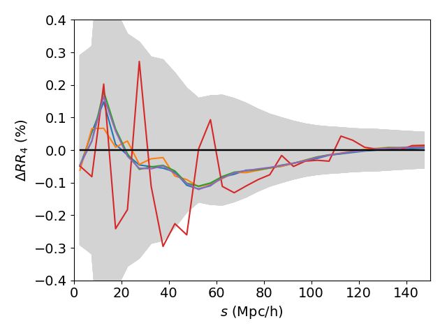
A&A 646, A40 (2021)

Nonetheless, to make the computation efficient, we can approx-                  There are three potential sources of error associated to the analyti-
imate this by taking the continuous limit on the sum and write it               cal pair count calculation: the p(r) estimation, the ω(θ) estimation,
out similarly as we do for the RR case:                                         and the precision on numerical integrals. In our methodology, the
                                                                                error level associated to each source is controlled respectively by
                                                                                the binning in p(r), angular map resolution nside, and ε. In the last
                                     Z rmax                Z smax
DR(smin , smax , µmin , µmax ) = 8π2        r12 n1 (r1 ) ×        s2            case however, we note that different algorithms can yield slightly
                                           rmin               smin
                           Z   µ∗max                                            different results even if ε is very small.
                       ×               n2 (r2 )ωDR (φ)dr1 dsdµ,          (21)        Regarding the performances of the RR implementation, for
                           µ∗min                                                the two considered surveys and considering 6000 bins in (s, µ),
                                                                                the full RR(s, µ) based on Eq. (12) takes about 5−20 min on a
where the angular cross-correlation function, ωDR , can be writ-                single CPU using the cuba library, even for ε ≈ 10−6 (gsl takes
ten as ωDR = hW1 W2 i, with W1 as a pixelated map containing                    significantly more time when ε < 10−3 ). In principle, we gain an
(weighted) source counts and W2 as the angular selection func-                  additional factor of two when using the pair line-of-sight mid-
tion as in Sect. 2.1. In this case, the normalisation on W1 and W2              point definition, as in that case, there is a symmetry along the
                                                            hW1 W2 i
does not matter since the final result is proportional to hW  1 ihW2 i
                                                                       .        line of sight for auto-correlation and we only need to compute
In principle, Eq. (21) should be close to Eq. (20) when the p(r)                µ > 0 pairs. The run time depends on the number of bins in (s, µ)
is fine enough to faithfully reproduce data radial overdensities.               but also in principle, on the shape of the integrand, as for com-
                                                                                plex p(r) or ω(θ), the integrals will take more time to converge
                                                                                (although, in our case, we did not see any noticeable difference).
3. Application                                                                  For the RR multipole moments in Eq. (14), the calculation only
                                                                                takes about 5 s with cuba algorithms using 30 bins in s, inde-
In this section, we apply our formalism for RR and DR pair                      pendently of the adopted value of ε.
counts to the case of BOSS and VIPERS redshift surveys and                           Regarding DR, the run times for the approximation in
test its accuracy.                                                              Eq. (21) are similar to those for RR by definition. However, the
                                                                                evaluation of Eq. (20) leads to large computational times of up
3.1. Numerical implementation                                                   to several weeks on a single CPU for large datasets. The run
                                                                                times scale linearly with the number of objects in the data sam-
The method takes as input the radial distance distribution of                   ple. In that case, direct data-random pair counting might be more
sources and the correlation function of the angular selection                   efficient.
function. To compute the latter, we first produce a Healpix                          The C code that follows this implementation is publicly
(Górski et al. 2005) full-sky map from the survey angular mask,                 available2 . It can be used with any input p(r) and ω(θ) to pre-
which is generally in form of a list of distinct spherical poly-                dict RR or DR pair counts.
gons with associated weights. We infer the angular correlation
function from the maps using Polspice (Szapudi et al. 2001;
 Chon et al. 2004), which takes advantage of Healpix isolati-                   3.2. Survey selection functions
tude pixelation scheme to quickly evaluate the angular correla-                 We consider two realistic redshift survey selection functions,
tion function ω(θ) with fast spherical harmonic transforms. The                 those of SDSS-BOSS DR12 CMASS (Alam et al. 2015) and
CPU time to compute the angular correlation function depends                    VIPERS PDR2 (Scodeggio et al. 2018) galaxy samples. We use
on the map resolution, but it is generally quite efficient. The map             the public galaxy catalogues3 and associated angular masks.
resolution is controlled by the nside1 parameter. For instance,                 Those two samples have complementary properties and thus
for BOSS it takes 3, 20 and 130 min on a single CPU for                         allow testing the method in different conditions. Indeed, while
nside = 2048, 4096, and 8192, respectively. For VIPERS, it takes                BOSS survey is wide and has a low galaxy number density,
6, 40, and 320 min for nside = 8192, 16384, and 32768, respec-                  VIPERS is much narrower and denser. Each survey is composed
tively. We note that we compute the angular power spectra until                 of two separated fields on the sky but here we only consider the
`max = 3 × nside; it is possible to reduce the run time by reduc-               BOSS North Galactic Cap (NGC) and VIPERS W1 fields and
 ing `max . The main limitation is memory since this operation                  we focus on 0.5 < z < 0.75 and 0.7 < z < 1.2 redshift intervals
 needs to load the full-sky map, which can be difficult for high-               for BOSS and VIPERS, respectively.
 resolution maps. Once the correlation function of the angular                      The radial selection functions are shown in Fig. 1. The
Dmask,E average map value hWi, and average map squared value                    BOSS p(r) is estimated from the data by taking the histogram
  W 2 are computed, we can estimate the pair counts. This can                   of galaxy comoving distances and cubic-spline interpolating
be done by numerically evaluating the multi-dimensional inte-                   between the bins. In the case of VIPERS, we use the fitting func-
grals of Eqs. (12) and (20) (or (21)), respectively, for RR and                 tion for the redshift distribution given in de la Torre et al. (2013).
 DR. We tested different integration schemes, namely:                           We assumed two cosmologies to convert redshift to comoving
  – gsl (Gough 2009) integration algorithm cquad;                               distance: flat ΛCDM with Ωm = 0.31 and Ωm = 0.25 for BOSS
  – cuba library (Hahn 2005) set of optimised algorithms for                    and VIPERS, respectively. Nonetheless, the choice of fiducial
     multi-dimensional integration: vegas, suave, divonne and                   cosmology has no impact on the accuracy of the analytical
     cuhre.                                                                     predictions.
In each case, we need to specify a maximum tolerance on the                         The angular selection functions that we used for VIPERS
integral relative error ε. The gsl cquad algorithm only performs                W1 and BOSS NGC are presented in Appendix A. In total,
one-dimensional integrals, and we thus implement nested inte-                   the surface covered by the BOSS NGC (VIPERS W1) field is
grals with same ε to perform the full three-dimensional integral.
                                                                                2
                                                                                  http://github.com/mianbreton/RR_code
1
   The total number of pixels in a full-sky map is given by Npix = 12 ×         3
                                                                                  Available at http://data.sdss.org/sas/dr12/boss/lss/
nside2 .                                                                        (BOSS) and http://vipers.inaf.it/rel-pdr2.html (VIPERS).

A40, page 4 of 10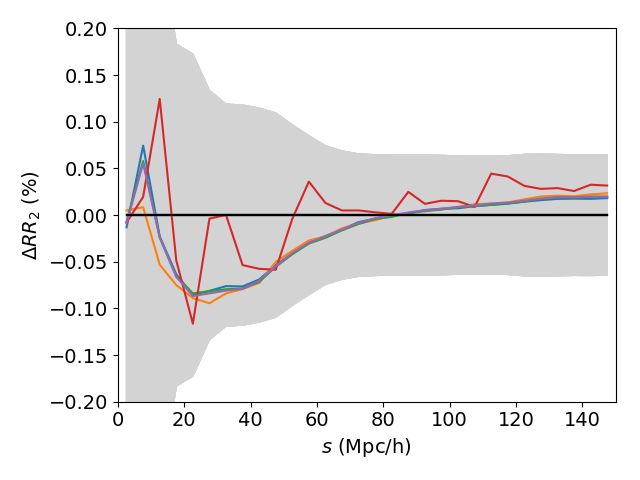
M.-A. Breton and S. de la Torre: Fast RR and DR calculation

Fig. 1. Adopted radial distance distribution p(r) for the BOSS NGC
CMASS sample at 0.5 < z < 0.75 (blue solid curve) and VIPERS
W1 sample at 0.7 < z < 1.2 (red dashed line). The distributions are           Fig. 3. Top panel: two-point correlation function of the VIPERS angular
normalised so that the integral is unity. The vertical solid (dashed) lines   selection function obtained from a Healpix map with nside = 65536.
show the adopted sample limits for BOSS (VIPERS).                             Bottom panel: relative difference on the angular two-point correlation
                                                                              function with respect to lower resolution maps, i.e. nside = 8192, 16834,
                                                                              32768 in blue, orange, and green curves, respectively.

Fig. 2. Top panel: two-point correlation function of the BOSS angu-
lar selection function obtained from a Healpix map with nside = 8192.
Bottom panel: relative difference on the angular two-point correlation
function with respect to lower resolution maps, i.e. nside = 2048, 4096
in blue and orange curves, respectively.

                                                                              Fig. 4. Detail of the VIPERS W1 angular mask showing the impact of
7427.4 deg2 (10.7 deg2 ). The angular selection function enters               Healpix resolution on the sampling of the survey angular mask.
in Eq. (12) through its auto-correlation function. The latter are
given in Figs. 2 and 3, respectively for BOSS and VIPERS.
    We test different map resolutions by varying the Healpix                  convergence of the angular correlation function with increasing
resolution parameter nside from 2048 to 8192. For BOSS, the                   nside, allows us to assess that resolutions of nside = 8192 and
correlation function is very smooth. The relative difference                  nside = 65536 are sufficiently accurate for BOSS and VIPERS
between nside = 2048, 4096 cases and nside = 8192 is roughly                  respectively. We note that while the map resolution impacts the
constant, at 0.1% and 0.05% respectively. In the case of VIPERS,              estimation of the angular selection function two-point correla-
the angular mask has more small-scale features but similarly, the             tion function, it also changes the estimation of n(r) through hWi,
relative differences between angular correlation functions based              which partly compensates the bias from ω(θ) in the final RR and
on different map resolutions are nearly constant in scale. The                DR estimations.
bias is larger than in the BOSS case, with a relative difference
with respect to nside = 65536 of 4%, 2%, and 0.5%, respectively               3.3. RR counts
for nside = 8192, 16834, 32768. This difference is due to the
fact that we need a significantly higher map resolution to cor-               We compare our analytical prediction for RR with the aver-
rectly account for the angular selection function as illustrated in           age random-random counts hRRi, obtained from 100 random
Fig. 4. The latter figure shows a detail of the VIPERS angular                samples constructed using the same radial and angular selec-
mask pixelated at nside = 8192 and nside = 65536. Overall, the                tion functions. Within the considered redshift intervals, there
                                                                                                                                    A40, page 5 of 10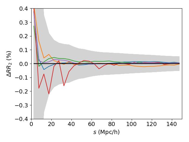
A&A 646, A40 (2021)
are 435185 BOSS and 24316 VIPERS galaxies and we gener-
ate 3 × 10⁷ and 3.9 × 10⁶ points per random sample, respectively
(i.e. multiplicative factors of about 70 and 160 with respect to
the data) with the radial distributions shown in Fig. 1. We com-
pute the pair counts from the random samples using the fast
Corrfunc pair-counting code (Sinha & Garrison 2020). Our
method predicts anisotropic RR(s, µ) counts, but to simplify the
comparison, we consider the first three even multipoles, that is,
RR` (s) = (2` + 1)/2 i RR(s, µi )L` (µi )∆µ with ` = 0, 2, 4, where
P
linear bins µi extend from −1 to 1. Those comparisons are pre-
sented in Fig. 5 for BOSS and in Fig. 6 for VIPERS. We see
that for both surveys, the relative difference between the ana-
lytical computation and hRRi is well within the variance of the
random samples. We compare the results obtained with different
numerical integration algorithms (see figure insets and Sect. 3.1)
and find that cuhre tends to depart from the others algorithms,
which is understandable since it is intrinsically different from
the others. If we ignore cuhre, we see that, at most, the relative
difference between the analytical computation and hRRi remains
within 3 × 10⁻⁵ for BOSS and 1.7 × 10⁻⁴ for VIPERS on the
monopole, and about 10−3 for the quadrupole and hexadecapole
for both surveys.
The variance on the random sample counts depends on the
number of points in the sample and, thus, we may ask what is the
number of random points needed to achieve the same accuracy
as in the analytical method. Keihänen et al. (2019) showed that
the relative variance on RR in a given bin is:
( " t # )
2 G 1
var(RR) = 2(Nr − 2) − 1 + p − 1 , (22)
Nr (Nr − 1) (G p )2 G
with Nr the number of random points, and G p , Gt terms are
(Landy & Szalay 1993):
hnp i
Gp = , (23)
Nr (Nr − 1)/2
hnt i
Gt = , (24)
Nr (Nr − 1)(Nr − 2)/2
with hnp i and hnt i the number of pairs and triplets averaged over
several realisations. While G p can easily be estimated from the
random samples, we directly solve for Gt from the estimated
var(RR). We can then deduce which Nr give standard deviations
similar to 3 × 10⁻⁵ and 1.7 × 10⁻⁴ for the monopole. We found
that we need an additional factor of at least 20(10) for BOSS
(VIPERS) in the number of random points. Therefore, the ana-
lytical method allows the achievement of the same accuracy as
by using a random sample with about 20 × 70 (10 × 160) more
points than data in BOSS (VIPERS). Finally, we note that cuba
integration algorithms have parameters that can be potentially
further fine-tuned to achieve better accuracy.
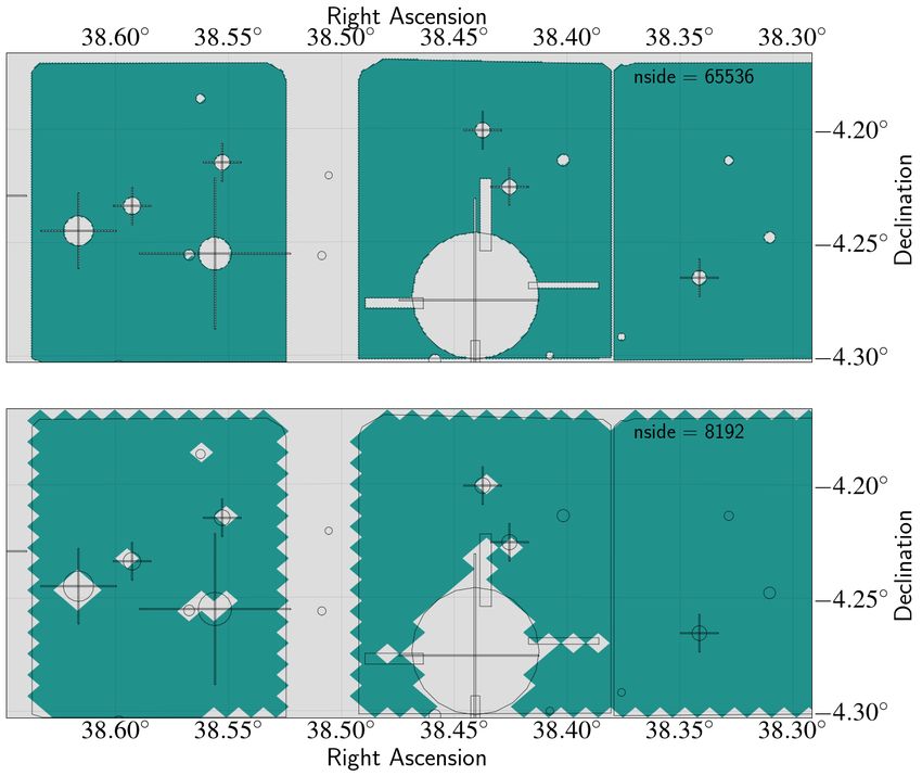
Fig. 5. Relative difference between the analytical and random
catalogue-based mean hRRi pair-count multipole moments (` = 0, 2,
3.4. DR counts 4, in the top, middle, and bottom panels, respectively) for BOSS. The
grey shaded area shows the standard deviation among the random cat-
In the DR case, we need to rely on approximations. Under the alogues, while blue, orange, green, red, and purple curves present the
approximation in Eq. (17), we have two possibilities to calculate relative differences obtained with vegas, suave, divonne, cuhre, and gsl
DR counts: either a discrete sum over all source distances as in algorithms, respectively, when using ε = 10−5 .
Eq. (20) or by further approximating the discrete sum by an inte-
gral as in Eq. (21). In the last case, we can already anticipate that
the results will depend on the input p(r1 ), particularly its ability to Eq. (20). For the random part we use in p(r2 ) the distributions
to reproduce line-of-sight structures in the data. In Figs. 7 and 8, provided in Fig. 1. It is worth noting that we use cubic splines to
we show different estimations of the data p(r1 ) in VIPERS and model the data distributions in Figs. 7 and 8. While other ways
BOSS, varying the bin size in r1 . In the limit where p(r1 ) resem- of estimating p(r1 ) could have been chosen, we only focus on
bles a sum of Dirac delta functions, Eq. (21) should be equivalent the relative importance of the binning, and therefore, the method
A40, page 6 of 10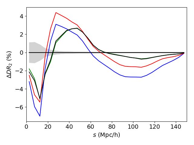
M.-A. Breton and S. de la Torre: Fast RR and DR calculation

                                                                         Fig. 7. Estimated radial distance distribution p(r) in the VIPERS sample
                                                                         at 0.7 < z < 1.2 using different linear bin size in r. The distributions
                                                                         are normalised so that the integral is unity. The blue dotted-dashed, red
                                                                         dashed, and black solid lines are the distributions obtained when using
                                                                         large, intermediate, and small bin sizes, respectively.

                                                                         Fig. 8. Same as Fig. 7, but for BOSS.

                                                                         for the quadrupole and hexadecapole, as shown in Fig. 9. More-
                                                                         over, we see that the prescription in Eq. (21) leads to a system-
                                                                         atic bias of up to about 2% on the monopole when using a large
                                                                         binning in the input p(r1 ), but converges towards Eq. (20) result
                                                                         when a small binning is adopted, as expected.
                                                                             In the case of BOSS, we find similar trends but with an
Fig. 6. Same as Fig. 5, but for VIPERS.                                  higher accuracy, as shown in Fig. 10. We find at most a dif-
                                                                         ference of 5 × 10⁻⁴ on the monopole between the analytical
                                                                         solution, either Eqs. (20) or (21) with a fine p(r1 ), and direct
                                                                         pair counting. Regarding the quadrupole and hexadecapole, the
used for the estimation is irrelevant here (however, it would be         relative difference is about 1%. Here, the approximation in
necessary for an accurate, in-depth characterisation of the radial       Eq. (17) is more appropriate since the data sample is larger.
selection function).                                                     This explains the improved accuracy that is reached. We empha-
    Following the same methodology as in Sect. 3.3, we com-              sise that the variance in Figs. 9 and 10 only comes from the
pute hDRi for both surveys using the same data catalogue and             random samples since a single data catalogue is used. There-
100 random samples, which we later compare to the predictions            fore, increasing the number of random points would reduce this
based on Eqs. (20) and (21) using different input data p(r1 ). In        variance. Overall, because of the approximation in Eq. (17),
the case of VIPERS, we find that when using Eq. (20), the dis-           our analytical DR predictions remain biased, exceeding the typ-
crepancy between the analytical prediction and direct pair count-        ical variance introduced by random sampling in direct pair
ing is on the order of 1% for the monopole, up to several percent        counting.
                                                                                                                               A40, page 7 of 10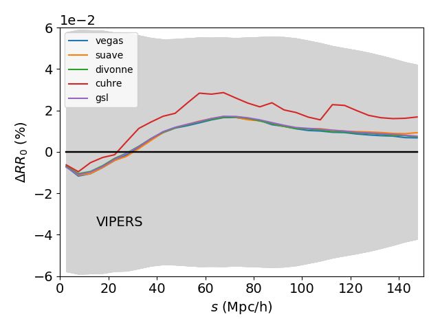
A&A 646, A40 (2021)

Fig. 9. Relative difference between the analytical and random               Fig. 10. Same as Fig 9 but for BOSS. Here. the prediction of Eq. (20)
catalogue-based mean hDRi multipoles (` = 0, 2, 4, in the top, mid-         in green is obtained with GSL using ε = 10−3 .
dle, and bottom panels, respectively) for VIPERS. The grey shaded area
shows the standard deviation among the random catalogues. The pre-
dictions use Eq. (17) and p(r) with large (blue), intermediate (red), and   DR. These expressions can be solved numerically in an efficient
small (black) bin sizes. These use vegas with ε = 10−5 . The green line     way. This method, which does not rely on generating random
shows the prediction of Eq. (20) obtained with GSL using ε = 10−4 .         mocks, only takes as input the comoving radial distance distribu-
                                                                            tion in an assumed cosmology and the angular selection function
4. Conclusion                                                               two-point correlation function, which only needs to be estimated
                                                                            a single time for a given survey. Once those quantities are pro-
In this paper, we present general analytical expressions for the            vided, the full computation takes about a few minutes to obtain
random-random and data-random pair counts in the case of a                  anisotropic pair counts RR(s, µ) and a few seconds for its mul-
realistic survey geometry. The main results are given in Eqs. (12)          tipole moments, using a single CPU and standard libraries for
(or (14) for the multipole moments) for RR and in Eq. (21) for              three-dimensional integration.
A40, page 8 of 10
M.-A. Breton and S. de la Torre: Fast RR and DR calculation
We tested this method in the context of the BOSS and References
VIPERS survey geometries and found excellent agreements with Alam, S., Albareti, F. D., Allende Prieto, C., et al. 2015, ApJS, 219, 12
expected RR pair counts. The predicted counts exhibit a high Alam, S., Ata, M., Bailey, S., et al. 2017, MNRAS, 470, 2617
accuracy for the cases investigated in this work, equivalent to Alonso, D. 2012, ArXiv e-prints [arXiv:1210.1833]
that we would obtain by performing pair counting in random Bautista, J. E., Paviot, R., Vargas Magaña, M., et al. 2021, MNRAS, 500, 736
samples of about 1400−1600 more random points than data in Beutler, F., Seo, H.-J., Saito, S., et al. 2017, MNRAS, 466, 2242
Bianchi, D., & Percival, W. J. 2017, MNRAS, 472, 1106
those surveys for the monopole. The main advantage is that the Blake, C., Brough, S., Colless, M., et al. 2012, MNRAS, 425, 405
method is fast and does not rely on any spatial sampling, while Castorina, E., Hand, N., Seljak, U., et al. 2019, JCAP, 2019, 010
usually we need to generate a random catalogue with at least 50 Chon, G., Challinor, A., Prunet, S., Hivon, E., & Szapudi, I. 2004, MNRAS, 350,
times the number of objects in the data. We believe that this can 914
Cole, S., Percival, W. J., Peacock, J. A., et al. 2005, MNRAS, 362, 505
be of some use for future surveys with large data samples and Davis, M., & Peebles, P. J. E. 1983, ApJ, 267, 465
very expensive RR pair count calculations. Dawson, K. S., Schlegel, D. J., Ahn, C. P., et al. 2013, AJ, 145, 10
The DR pair counts can also be calculated analytically based de la Torre, S., Guzzo, L., Peacock, J. A., et al. 2013, A&A, 557, A54
on certain approximations. We found that the results are slightly Demina, R., Cheong, S., BenZvi, S., & Hindrichs, O. 2018, MNRAS, 480, 49
biased with respect to the expected counts. For VIPERS and DESI Collaboration (Aghamousa, A., et al.) 2016, ArXiv e-prints
[arXiv:1611.00036]
BOSS, we found a bias with respect to direct pair counts of 1% eBOSS Collaboration (Alam, S., et al.) 2020, ArXiv e-prints
and 0.05%, respectively, for the monopole, up to several percents [arXiv:2007.08991]
on the quadrupole and hexadecapole. This bias should decrease Eisenstein, D. J., Weinberg, D. H., Agol, E., et al. 2011, AJ, 142, 72
with the increasing number of data points. When estimating DR Feldman, H. A., Kaiser, N., & Peacock, J. A. 1994, ApJ, 426, 23
Garilli, B., Guzzo, L., Scodeggio, M., et al. 2014, A&A, 562, A23
for several data samples, we need to compute, for each sample, Górski, K. M., Hivon, E., Banday, A. J., et al. 2005, ApJ, 622, 759
its angular two-point correlation function with respect to the sur- Gough, B. 2009, GNU Scientific Library Reference Manual (Network Theory
vey angular selection function. Ltd.)
Overall, the method presented in this paper for efficiently Guzzo, L., Pierleoni, M., Meneux, B., et al. 2008, Nature, 451, 541
evaluating the survey window two-point function should be very Guzzo, L., Scodeggio, M., Garilli, B., et al. 2014, A&A, 566, A108
Hahn, T. 2005, Comput. Phys. Commun., 168, 78
useful when dealing with massive galaxy surveys. The formulae Hahn, T. 2015, J. Phys. Conf. Ser., 608, 012066
provided are fast in terms of the speed of the evaluation. With Hamilton, A. J. S. 1993, ApJ, 417, 19
further efficient parallelisation (e.g., Hahn 2015), we should be Hearin, A. P., Campbell, D., Tollerud, E., et al. 2017, AJ, 154, 190
able to compute RR and DR in an extremely small amount of Hewett, P. C. 1982, MNRAS, 201, 867
Jarvis, M., Bernstein, G., & Jain, B. 2004, MNRAS, 352, 338
time. In that case, we could imagine RR and DR being evaluated Kaiser, N. 1987, MNRAS, 227, 1
in different cosmologies at each step of a cosmological likeli- Keihänen, E., Kurki-Suonio, H., Lindholm, V., et al. 2019, A&A, 631, A73
hood analysis. This opens up new horizons for the way we anal- Landy, S. D., & Szalay, A. S. 1993, ApJ, 412, 64
yse galaxy survey data in the future. Laureijs, R., Amiaux, J., Arduini, S., et al. 2011, ArXiv e-prints
[arXiv:1110.3193]
Maddox, S. J., Efstathiou, G., & Sutherland, W. J. 1996, MNRAS, 283, 1227
Acknowledgements. We thank Eric Jullo for his help on dealing with par- Marulli, F., Veropalumbo, A., & Moresco, M. 2016, Astron. Comput., 14, 35
tial, high-resolution Healpix maps and his comments on the draft. We thank Moore, A. W., Connolly, A. J., Genovese, C., et al. 2001, in Mining the Sky, eds.
the Instituto de Astrofísica de Andalucía (IAA-CSIC), and the Spanish aca- A. J. Banday, S. Zaroubi, & M. Bartelmann, 71
demic and research network (RedIRIS, http://www.rediris.es) in Spain Mueller, E.-M., Percival, W. J., & Ruggeri, R. 2019, MNRAS, 485, 4160
for providing the skun@IAA_RedIRIS server that allowed us to run the cal- Peacock, J. A., Cole, S., Norberg, P., et al. 2001, Nature, 410, 169
culations for high-resolution nside = 65535 maps. This work has been carried Peebles, P. J. E., & Hauser, M. G. 1974, APJS, 28, 19
out thanks to the support of the OCEVU Labex (ANR-11-LABX-0060) and Percival, W. J., Reid, B. A., Eisenstein, D. J., et al. 2010, MNRAS, 401, 2148
of the Excellence Initiative of Aix-Marseille University – A*MIDEX, part of Ross, A. J., Beutler, F., Chuang, C.-H., et al. 2017, MNRAS, 464, 1168
the French ‘Investissements d’Avenir’ programme. Funding for SDSS-III has Samushia, L., Percival, W. J., & Raccanelli, A. 2012, MNRAS, 420, 2102
been provided by the Alfred P. Sloan Foundation, the Participating Institu- Sánchez, A. G., Scoccimarro, R., Crocce, M., et al. 2017, MNRAS, 464,
tions, the National Science Foundation, and the U.S. Department of Energy 1640
Office of Science. The SDSS-III website is http://www.sdss3.org/. SDSS- Scodeggio, M., Guzzo, L., Garilli, B., et al. 2018, A&A, 609, A84
III is managed by the Astrophysical Research Consortium for the Participating Sinha, M., & Garrison, L. H. 2020, MNRAS, 491, 3022
Institutions of the SDSS-III Collaboration including the University of Arizona, Slepian, Z., & Eisenstein, D. J. 2016, MNRAS, 455, L31
the Brazilian Participation Group, Brookhaven National Laboratory, Carnegie Strauss, M. A., Davis, M., Yahil, A., & Huchra, J. P. 1992, ApJ, 385, 421
Mellon University, University of Florida, the French Participation Group, the Szapudi, I., Prunet, S., Pogosyan, D., Szalay, A. S., & Bond, J. R. 2001, ApJ,
German Participation Group, Harvard University, the Instituto de Astrofisica de 548, L115
Canarias, the Michigan State/Notre Dame/JINA Participation Group, Johns Hop- Tegmark, M., Eisenstein, D. J., Strauss, M. A., et al. 2006, Phys. Rev. D, 74,
kins University, Lawrence Berkeley National Laboratory, Max Planck Institute 123507
for Astrophysics, Max Planck Institute for Extraterrestrial Physics, New Mexico Vogeley, M. S., Park, C., Geller, M. J., & Huchra, J. P. 1992, ApJ, 391, L5
State University, New York University, Ohio State University, Pennsylvania State Wilson, M. J., Peacock, J. A., Taylor, A. N., & de la Torre, S. 2017, MNRAS,
University, University of Portsmouth, Princeton University, the Spanish Partic- 464, 3121
ipation Group, University of Tokyo, University of Utah, Vanderbilt University, Yamamoto, K., Nakamichi, M., Kamino, A., Bassett, B. A., & Nishioka, H. 2006,
University of Virginia, University of Washington, and Yale University. PASJ, 58, 93
A40, page 9 of 10A&A 646, A40 (2021)
Appendix A: VIPERS and SDSS-BOSS survey associating fibres to potential spectroscopic targets in the survey.
footprints We use this quantity as a weight in defining the angular selection
function. In the case of VIPERS, the angular selection function is
In Figs. A.1 and A.2, we provide the footprints and angular taken to be unity inside the spectroscopic mask (quadrant-shaped
masks for VIPERS W1 and SDSS-BOSS CMASS NGC fields, polygons) and null otherwise, except in the regions of the pho-
respectively, which we used in this analysis. In the case of BOSS tometric mask (circular- and star-shaped polygons), where it is
angular mask, each distinct mask polygon has an associated also set to zero.
tiling success rate, which is a measure of the completeness in
Fig. A.1. VIPERS W1 footprint.
Fig. A.2. BOSS CMASS NGC footprint.
A40, page 10 of 10You can also read