PID Tuning Guide A Best-Practices Approach

PID Tuning Guide
      A Best-Practices Approach
to Understanding and Tuning PID Controllers

                     First Edition
              by Robert C. Rice, PhD

          Technical Contributions from:

 Also Introducing: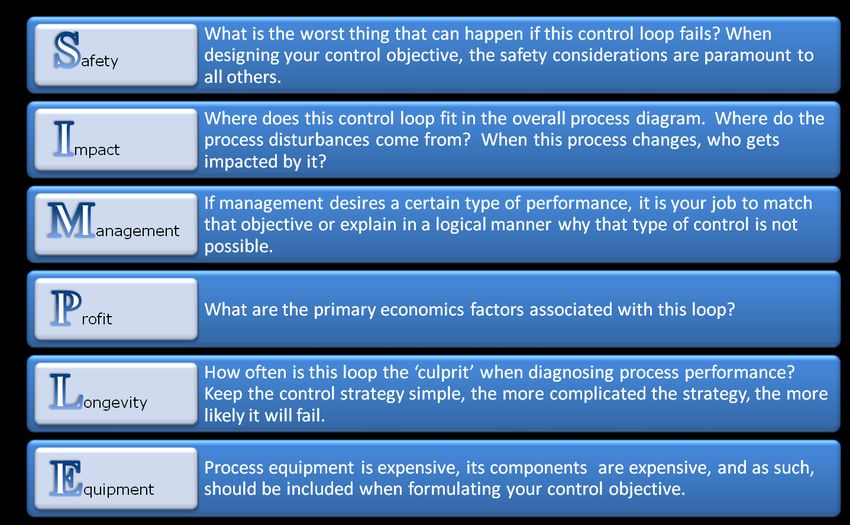

Table of Contents                                                                              2

Forward                                                                                        3

The PID Controller and Control Objective                                                       4

Testing: Revealing a Process’ Dynamics                                                         6

Control Station’s NSS Modeling Innovation                                                      9

Data Collection: Speed is Everything                                                           10

The FOPDT Model: The Right Tool for the Job                                                    12

Is Your Process Non-Integrating or Integrating?                                                13

Process Gain: The ―How Far‖ Variable                                                           14

Time Constant: The ―How Fast‖ Variable                                                         16

Dead-Time: The ―How Much Delay‖ Variable                                                       18

Changing Dynamic Process Behavior                                                              19

The Basics of PID Control                                                                      20

Rules of Thumb: PID Controller Configurations                                                  21

Using and Calculating the PI Controller Tuning Parameters                                      22

Notes Concerning Specific NovaTech D/3 PID Algorithms                                          24

Introducing D/3 Loop Optimizer Powered by Control Station                                      26

Copyright © 2010 Control Station, Inc. All Rights Reserved.
Control Station, the Control Station logo, the D/3 Loop Optimizer logo, and the NSS Modeling
Innovation are either registered trademarks or trademarks of Control Station Incorporated in
the United States and/or other countries. All other trademarks are the property of their
respective owners.

Forward                                                    3

Tuning PID controllers can seem a mystery. Parameters
that provide effective control over a process one day fail to
do so the next. The stability and responsiveness of a
process seem to be at complete odds with each other. And
controller equations include subtle differences that can
baffle even the most experienced practitioners. Even so,
the PID controller is the most widely used technology in
industry for the control of business-critical production
processes and it is seemingly here to stay.

This guide offers a ―best-practices‖ approach to PID
controller tuning. What is meant by a ―best-practices‖
approach? Basically, this guide shares a simplified and
repeatable procedure for analyzing the dynamics of a
process and for determining appropriate model and tuning
parameters. The techniques covered are used by leading
companies across the process industries and they enable
those companies to consistently maintain effective and safe
production environments. What’s more, they’re techniques
that are based on Control Station’s Practical Process Control
– a comprehensive curriculum that has been used to train
over a generation of process control professionals.

Our guide provides the fundamentals – a good starting
point for improving the performance of PID controllers. It
offers an introduction to both the art and the science
behind process control and PID controller tuning. Included
are basic terminology, steps for analyzing process
dynamics, methods for determining model parameters, and
other valuable insights.     With these fundamentals we
encourage you to investigate further and fully understand
how to achieve safe and profitable operations. As I shared,
the PID controller appears here to stay.

Robert C. Rice, PhD
Control Station, Inc.

The PID Controller and Control Objective                   4

Through use of the Proportional-Integral-Derivative (PID)
controller, automated control systems enable complex
production process to be operated in a safe and profitable
manner. They achieve this by continually measuring
process operating parameters such as Temperature,
Pressure, Level, Flow, and Concentration, and then by
making decisions to open or close a valve, slow down or
speed up a pump, or increase or decrease heat so that
selected process measurements are maintained at the
desired values.    The overriding motivation for modern
control systems is safety. Safety encompasses the safety
of people, the safety of the environment, as well as the
safety of production equipment. The safety of plant
personal and people in the surrounding community should
always be the highest priority in any plant operation.

Good control is subjective. One engineer’s concept of good
control can be the epitome of poor control to another. In
some facilities the ability to maintain operation of any loop
in automatic mode for a period of 20 minutes or more is
considered good control. Although subjective, we view
good control as an individual control loop’s ability to
achieve and maintain the desired control objective. But
this view introduces an important question: What is the
―control objective‖?

It can be argued that knowing the control objective is the
single most important piece of information in designing and
implementing an effective control strategy. Understanding
the control objective suggests that the engineering team
has a firm grasp of what the process is designed to
accomplish. This must be the case whether the goal is to
fill bottles to a precise level, maintain the design
temperature of a highly exothermic reaction without
blowing up, or some other objective. Truly the control
objective involves this and more.

The PID Controller and Control Objective                                    5

 Shown on the right is a typical surge
 tank. Surge tanks are used to
 minimize disturbances to other
 downstream production processes.
 They         are      usually       tuned
 c o ns e r v ativ e ly , a llo w in g the
 Measured Variable to drift above and
 below set point without exceeding
 the upper or lower alarms limits. In
 most cases, tight control over a
 surge tank is counterproductive as
 tight control does not adequately
 insulate other production processes
 from disturbances.

                                     Shown on the left is a steam drum.
                                     Steam drums act as a reservoir of
                                     water and/or steam for boiler
                                     systems. They are typically
                                     engineered with very tight tolerances
                                     around set point in order to maintain a
                                     specific level of steam production.
                                     Variation of the level is detrimental to
                                     the process’ efficiency and
                                     productivity.

Testing: Revealing a Process’ Dynamics                      6

The best way to learn about the dynamic behavior of a
process is to perform tests. Even though open loop (i.e.
manual mode) tests provide the best data, tests also can be
performed successfully in closed loop (i.e. automatic mode).
The goal of a test is to move the controller output (OT) both
far enough and fast enough so that the dynamic character
of the process is revealed through the response of the
Measured Variable (ME). As shared previously, the dynamic
behavior of a process usually differs from operating range to
operating range, so be sure to test when the Measured
Variable is near the value for normal operation of the
process.

Production processes are inherently noisy. As a result,
process noise is typically visible in the data, showing itself
as random chatter.        It must be considered prior to
conducting a test. If the test performed is not sufficient in
magnitude, then it is quite possible that process noise will
mask the dynamics – completely or partially – and prevent
effective tuning. To generate a reliable process model and
effective tuning parameters, it is recommended that only
tests that are 5-10 times the size of the noise band be
performed.

Disturbances represent another important detail that must
be considered when performing tests.           A good test
establishes a clear correlation between the planned change
in controller output with the observed change in measured
Variable. If process disturbances occur during testing, then
they may influence the observed change in the measured
Variable. The resulting test data would be suspect and, as
a result, additional testing should be performed.

There are a variety of tests that are commonly performed
in industry. They include the Step, Pulse, Doublet, and
Pseudo Random Binary Sequence. Examples of each are
shown on the following page.

Testing: Revealing a Process’ Dynamics         7

Step Test – A step test is when the
controller output is ―stepped‖ from one
constant value to another. It results in
the measured Variable moving from one
steady state to a new steady state.
Unfortunately, the step test is simply too
limiting to be useful in many practical
applications. The drawback is that it takes
the process away from the desired
operating level for a relatively long period
of time which typically results in
significant off-spec product that may
require reprocessing or even disposal.

Pulse Test – A pulse test can be thought
of as two step tests performed in rapid
succession. The controller output is
stepped up and, as soon as the measured
variable shows a clear response, the
controller output is then returned to its
original value. Ordinarily, the process
does not reach steady state before the
return step is made. Pulse tests have the
desirable feature of starting from and
returning to an initial steady state.
Unfortunately, they only generate data on
one side of the process’ range of
operation.

Doublet Test – A doublet test is two
pulse tests performed in rapid succession
and in opposite directions. The second
pulse is implemented as soon as the
process has shown a clear response to the
first pulse. Among other benefits, the
doublet test produces data both above
and below the design level of operation.
For    this   reason,  many     industrial
practitioners find the doublet to be the
preferred test method.

PRBS Test – A pseudo-random binary
sequence (PRBS) test is characterized by
a sequence of controller output pulses
that are uniform in amplitude, alternating
in direction, and of random duration. It is
termed "pseudo" as true random behavior
is   a    theoretical   concept  that    is
unattainable by computer algorithms. The
PRBS test permits generation of useful
dynamic process data while causing the
smallest maximum deviation in the
measured variable from the initial steady
state.

Testing: Revealing a Process’ Dynamics                      8

When performing tests and evaluating results, consider the
following three(3) questions:

1. Was the process at a relative “steady state” before
the test was initiated?

Beginning at steady state simplifies the process of
determining accurate model and tuning parameters. It
allows for a clear relationship between the change in
controller output and the associated response from the
manipulated measured variable to be demonstrated. Said
another way, it eliminates concern that test results may
have been compromised by other non-test-related
dynamics within the process. This is true when calculating
model and tuning parameters by hand as well as when
using most tuning software tools.

2. Did the dynamics of the test clearly dominate any
apparent noise in the process?

It is important that the change in either controller output or
set point cause a response that clearly dominates any
process noise. To meet this requirement, the change in
controller output should force the measured variable to
move at least 5-10 times the noise band. By doing so, test
results will be easier to analyze.

3. Were disturbances absent during testing?

It is essential that test data contain process dynamics that
were clearly – and in the ideal world exclusively – forced by
changes in the controller output. Dynamics resulting from
other disturbances – known or unknown – will undermine
the accuracy of the subsequent analysis. If you suspect
that a disturbance corrupted the test, it is conservative to
rerun the test.

Control Station’s NSS Modeling Innovation                             9

Traditional ―state-of-the-art‖ process modeling and tuning
tools require steady-state operation before conducting
tests. Failure to achieve or maintain steady-state operation
during these tests impairs the efficacy of the model
parameters produced by such tools. Depending on the
process involved, the impact of sub-optimal model
parameters can be significant in terms of associated
increases in production cost, reduction of production
throughput, compromising of production quality, and
overall undermining of production safety.
Control Station’s NSS Model Fitting Innovation applies a
unique method for modeling dynamic process data and
does not require steady-state operation prior to performing
tests.    As a result, the innovation offers significant
advantage over other modeling and tuning technologies.
The NSS Model Fitting Innovation does not utilize a specific
data point or average data point as a ―known‖ and is
therefore not constrained by it. Rather, the NSS Model
Fitting Innovation centers the model across the entire range
of data under consideration.        Since no data point is
weighted disproportionately in the calculation and
minimization of Error, the innovation is free to consider all
possible model adjustments and to optimize the model’s fit
relative to all of the data under analysis.
                                      Shown on the left is a trend
                                      depicting    the   model      fit
                                      produced by traditional PID
                                      tuning software.   The process
    Traditional Modeling Software
                                      is in the midst of a transition,
                                      preventing the software from
                                      accurately    describing     the
                                      process’ dynamic behavior.
 Shown on the right is a trend of
 the same process data and the
 corresponding model generated
 with D/3 Loop Optimizer. Even
 though   in   the   midst   of   a
 transition, D/3 Loop Optimizer       D/3 Loop Optimizer
 accurately models the dynamic
 behavior and produces effective
 tuning parameters.

Data Collection: Speed is Everything                                      10

When using software to model a process and tune the
associated PID controller, be aware that the data collection
speed is as important as any other aspect of the test. As
shared previously, a good test should be plain as day – it
should start at steady state and show a response that is
distinct from any noise that may exist in the process. But if
data is not collected at a fast enough rate, the software will
be unable to provide an accurate model and in all likelihood
the effort to tune the controller will fail.

They say a broken watch is right twice a day. Now imagine
a highly oscillatory process that swings 15% above and
below set point every minute. That same process would be
at the desired set point twice each minute – every 30
seconds or so. If data for this process is captured every 30
seconds, it is possible that the data would show a flat line
and suggest that the process is under perfect control. That
data collection rate is clearly not fast enough to provide
adequate resolution.

Data should be collected at a minimum of ten (10) times
faster than the rate of the Process Time Constant. To be
clear, if the Process Time Constant is 10 seconds, then data
should be collected no slower than once per second. That
will assure that sufficient resolution is captured in the data.
Basic recommendations for data collect speed are listed
below:

   Process Type              Recommended Sample Rate

   Flow, Pressure           Less than 2 Seconds is Desirable

                      Between 1-5 Seconds Depending on Tank Size
        Level
                      (i.e. the smaller the tank, the faster the sample

  Fast Temperature               Between 5-15 Seconds

   Slow Tempera-
                                 Between 15-30 Seconds
        ture

  pH, Concentration              Between 5-30 Seconds

Data Collection: Speed is Everything                                  11

Shown below are a pair of real-world examples where the
data collection rates were too slow and the information
insufficient for tuning.
  Measured
                variable
  Controller
                Output

The first example shows a trend depicting a series of changes to valve
position and their associated impact. The data was taken directly from
the plant’s data historian. As the arrows point out, the data suggests
that the measured variable started to change before the valve’s
position was adjusted. That is either a sign of a very smart and psychic
process or one where the data doesn’t adequately tell the story.
   Measured
   Controller
                 Output

The second example involves a flow loop where data was collected at a
rate of 30 seconds. When trying to assess the dynamic behavior of a
process, it is important to have access to data that is collected fast
enough so that the shape of the response is visible. In this case, data
from the plant’s historian only shows the starting and ending points
associated with the increases to controller output. Absent is any truly
useful information related to the process’ dynamic behavior.

The FOPDT Model: The Right Tool for the Job             12

Success in controller tuning largely depends on successfully
deriving a good model from bump test data. The First Or-
der Plus Dead-Time (FOPDT) model is the principal model –
or tool – used in tuning PID controllers. That requires an
explanation given that the FOPDT model is too simple for
time varying and non-linear process behavior.

Though only an approximation – for some processes a very
rough approximation – the value of the FOPDT model is
that it captures the essential features of dynamic process
behavior that are fundamental to control. When forced by
a change in the controller output, a FOPDT model reasona-
bly describes how the measured variable will respond. Spe-
cifically, the FOPDT model determines the direction, how
far, how fast, and with how much delay the measured vari-
able should respond with relative accuracy.

The FOPDT model is called "first order" because it only has
one (1) time derivative. The dynamics of real processes are
more accurately described by models that possess second,
third or higher order time derivatives. Even so, use of a
FOPDT model to describe dynamic process behavior is usu-
ally reasonable and appropriate for controller tuning proce-
dures. Practice has also shown that the FOPDT model is
sufficient for use as the model in more advanced control
strategies such as Feed Forward, Smith Predictor, and mul-
tivariable decoupling control.

The FOPDT model is comprised of three (3) parameters:
Process Gain, Process Time Constant, and Process Dead-
Time. The remaining portion of this guide will focus on
steps that can be followed to determine values for each of
these parameters. Once determined, the guide will intro-
duce tuning correlations with which tuning parameters can
be derived and used by the associated PID controller.

ob   Is Your Process Non-Integrating or Integrating?                13

     The plots below show idealized trends from two processes
     as they respond to a step test. The process on the left is
     non-integrating, also called self-regulating. The process on
     the right is integrating, also called non-self-regulating.
     Understanding the difference prior to modeling the process
     data is critical as applying the wrong model can have a
     significant effect on the tuning parameters         that are
     calculated. More importantly, choosing the wrong model
     can have a negative effect on your ability to control the
     process safely.

     A characteristic behavior of a non-integrating process is
     that it will naturally ―self-regulate‖ itself – it will transition
     to a new steady state over time. As shown in the trend,
     the process responds to the change in controller output and
     tapers off to a new steady state of operation.

     In contrast, an integrating process does not have a natural
     balance point. As shown in the trend, the process moves
     steadily in one direction after the change in controller
     output occurs.     The steady change associated with a
     integrating or non-self-regulating process will not stop until
     corrective action is taken.

Process Gain: The “How Far” Variable                      14

Process Gain is a model parameter that describes how
much the measured variable changes in response to
changes in the controller output. A step test starts and
ends at steady state, allowing the value of the Process Gain
to be determined directly from the plot axes. When viewing
a graphic of the step test, the Process Gain can be
computed as the steady state change in the measured
variable divided by the change in the controller output
signal that forced the change.

The formula for calculating Process Gain is relatively simple.
It is the change of the measured variable from one steady
state to another divided by the change in the controller
output from one steady state to another.

The strip chart below offer a graphic by which the Process
Gain can be determined. The graphic shows a 10% change
in the controller output – the output increases from 50% to
60%. The measured variable reacts to that change by
moving from a steady state value of ~2.0 meters to a new
steady state value of ~3.0 meters.

The graphic shows how the Process Gain from this example
should be calculated. The change in the measured variable
is equal to 1.0 meter (i.e. ~3.0 meters - ~2.0 meters = 1.0
meter). The change in controller output is equal to 10%
(i.e. 60% - 50% = 10%). Process Gain can then be
computed as 0.1 meters/percent.

Calculating Process Gain in Percent Span Units                   15

Process Gain is based on the same unit values that are
used in the process. These units are typically engineering
units such as flow rates (e.g. GPM, or gallons per minute),
temperature (e.g. °C, or degrees Celsius,), and pressure
(e.g. PSI, or pounds per square inch). It is important to
note that the controller does not use these engineering
units in its calculation. Instead, the controller uses the
percent span of signal. When using the Process Gain in
connection with the tuning correlations that follow, it is
important to convert this Process Gain into units that reflect
the manufactures' ―percent span‖.            This can be
accomplished by using the following formula:

MATH ALERT:

The process gain calculated on the previous page is from a
control loop that has a measured variable span of 0 to 10
meters, and a controller output span of 0 to 100%. To
convert this into the percent span units for use in the
controller tuning correlations, see the below formula:

                                m  100% ME  0% ME 100%OT  0%OT
 Process Gain [% Span] = 0.10                     
                                %OT    10m  0m    100%OT  0%OT
                              m 
 Process Gain [% Span] = 1.0 
                              %OT 

This Process Gain can be interpreted to mean that for every
1% that the controller output increases, the measured
variable will increase by 1% of its total span. This value in
percent span units should be between 0.5 and 2.5 for a well
designed process. Controller Gains above the 2.5 upper
limit are typically the result of a control valve or pump
being oversized for its particular application. Values for the
controller gain below the 0.5 lower limit are usually from an
over-spanned sensor.

Time Constant: The “How Fast” Variable                 16

The overall Process Time Constant describes how fast a
measured variable responds when forced by a change in
the controller output. Note that the clock that measures
speed does not start until the measured variable shows a
clear and visible response to the controller output step.
This is to distinguish the actual start for calculation
purposes from the time when the controller output is first
adjusted.

The Process Time Constant is equal to the time it takes
for the process to change 63.2% of the total change in
the measured variable. The smaller the time constant,
the faster the process.

Calculating Process Time Constant                        17

As shown in the strip charts below, begin by identifying
the time at which the measured variable first reacts to the
change in controller output – not the time when the
controller output first changes. In the example shown,
the measured variable shows a distinct change beginning
at approximately 4.1 minutes.

By estimating the total change in the measured variable,
it is then possible to determine a value equal to 63.2% of
the total change. In this case, the measured variable
moved from a value of ~1.85 meters to a value of ~2.85
meters. Therefore, 63.2% of the total change is ~0.6
meters (i.e. 2.85 meters – 1.85 meters = 1.0 meters x
0.632 = 0.6 meters). By adding 0.6 meters to the initial
value of the measured variable (i.e. 1.85), it is apparent
that the measured variable reaches the value of 2.45
meters at approximately 5.5 minutes.

The Process Time Constant is the difference between the
initial start of the change in the measured variable and
63.2% of the total change in the measured variable. In
this example, the initial value is 4.1 minutes and 63.2%
of the change occurs at 5.5 minutes. The Process Time
Constant is equal to 1.4 minutes.

Dead-Time: The “How Much Delay” Variable                  18

Process Dead-Time is the time that passes from the
moment the step change in the controller output is made
until the moment when the measured variable shows a
clear initial response to that change. Process Dead-Time
arises because of transportation lag and/or sample or
instrumentation lag. Transportation lag is defined as the
time it takes for material to travel from one point to
another. Similarly, sample or instrument lag is defined as
the time it takes to collect, analyze or process a
measured variable sample.
The larger the Process Dead-Time relative to the Process
Time Constant, the more difficult the associated process
will be to control. Typically speaking, as the Process
Dead-Time exceeds the Time Constant, the speed by
which the controller can react to any given change in that
same process is significantly decreased. That undermines
the PID controller’s ability to maintain stability. It is for
this reason that Process Dead-Time is often referred to as
the ―killer of control‖.
Calculating Process Dead-Time is relatively straight
forward. Begin by identifying the time at which the
controller output is changed. In the example provided,
the controller output is seen to change at a time of 3.8
minutes. Next, identify the time at which the measured
variable first reacts to the change in controller output.
When calculating the Process Time Constant it was
learned that the measured variable shows a distinct
change beginning at approximately 4.1 minutes. The
Process Dead-Time is then calculated as 0.3 minutes (i.e.
4.1 minutes - 3.8 minutes ).

e   Changing Dynamic Process Behavior                                   19

    In essence, the dynamic behavior of production processes
    can be characterized by how one variable responds over
    time to another variable. Understanding those dynamics
    allows the PID controller to maintain effective and safe
    control even in the face of disturbances. But gaining that
    understanding is not a trivial matter.

    Linear processes demonstrate the most basic dynamic
    behavior. They respond to disturbances in the same
    fashion regardless of the operating range. However, such
    processes are only linear for a period of time.         All
    processes have surfaces that foul or corrode, mechanical
    elements like seals or bearings that wear, feedstock
    quality or catalyst activity that drifts, environmental
    conditions such as heat and humidity that change, and
    other phenomena that impact dynamic behavior. The
    result is that linear processes behave a little differently
    with each passing day.

    Nonlinear processes demonstrate dynamic behavior that
    changes as the operating range changes.            Most
    production processes are nonlinear to one extent or
    another. With this understanding, nonlinear processes
    should therefore be tuned for use within a specific and
    typical operating range.

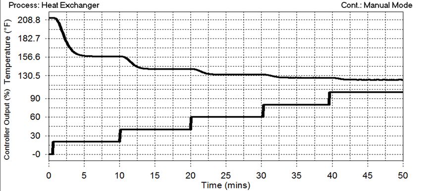
    The plot shown above depicts the nonlinear dynamics of a simple Heat
    Exchanger process. Notice how the controller output is stepped five (5)
    times in equal amounts of 20% but the response of the measured
    variables changes dramatically from the first to the last change.

The Basics of PID Control                                20

PID controllers are by far the most widely used family of
intermediate value controllers in the process industries.
As such, a fundamental understanding of the three (3)
terms – Proportional, Integral, and Derivative – that
interact and regulate control is worthwhile.

Proportional Term – The proportional term considers
―how far‖ the measured variable has moved away from
the desired set point. At a fixed interval of time, the
proportional term either adds or subtracts a calculated
value that represents error - the difference between the
process’ current position and the desired set point. As
that error value grows or shrinks, the amount added to or
subtracted from the error similarly grows or shrinks both
immediately and proportionately.

Integral Term – The integral term addresses ―how long‖
the measured variable has been away from the desired
set point. The integral term integrates or continually sums
up error over time. As a result, even a small error amount
of persistent error calculated in the process will aggregate
to a considerable amount over time.

Derivative Term – The derivative term considers ―how
fast‖ the error value changes at an instant in time. The
derivative computation yields a rate of change or slope of
the error curve. An error that is changing rapidly yields a
large derivative regardless of whether a dynamic event
has just begun or if it has been underway for some time.

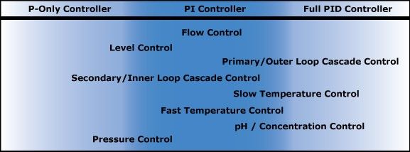
Rules of Thumb: PID Controller Configurations                            21

As a rule of thumb, no two processes behave the same.
They may produce the same product, utilize identical
instrumentation, and operate for the same period of time.
However, like identical children they will inevitably
develop unique characteristics.     Even so, production
processes do possess common attributes, and common
approaches to controlling them can be applied with great
success.

P-Only — P-Only control involves the exclusive use of the Proportional
Term. It is the simplest form of control which makes it the easiest to
tune. It also provides the most robust (i.e. stable) control. It provides an
initial and rapid kick in response to both disturbances and set point
changes, but it is subject to offset. P-Only control is suitable in highly
dynamic applications such as level control and in the inner loop of the
cascade architecture.

PI Control — PI is the most common configuration of the PID controller
in industry. It supplies the rapid initial response of a P-Only controller,
and it addresses offset that results from P-Only control. The use of two
(2) parameters makes this configuration relatively easy to tune.

PID Control — This configuration uses the full set of terms, including
the Derivative, and it allows for more aggressive Proportional and
Integral terms without introducing overshoot. It is good for use in
steady processes and/or processes that either respond slowly or have
little-to-no noise. The downfall of PID Control is its added complexity
and the increased chatter on the controller output signal. Increased
chatter typically results in excessive wear on process instrumentation
and increases maintenance costs.

The image below identifies each of the PID controller
configurations and suggests a configuration(s) for various
process types.

Using the PI Controller                                   22

Most industrial processes are effectively controlled using
just two of the PID controller’s terms – Proportional and
Integral. Although a detailed explanation is worthwhile, for
purposes of this guide it is hopefully sufficient to note that
the Derivative term reacts poorly in the face of noise. The
Derivative term may provide incremental smoothness to a
controller’s responsiveness, but it does so at the expense of
the final control element. Since most production processes
are inherently noisy, the Derivative term is frequently not
used.
PI controllers present challenges too. One such challenge
of the PI controller is that there are two tuning parameters
that can be adjusted. These parameters interact – even
fight – with each other. The graphic on the right shows how
a typical set point response might vary as the two tuning
parameters change.
The tuning map below shows how differences in Gain and
Reset Time can affect a PI controller’s responsiveness. The
center of the map is labeled as the base case.       As the
terms are adjusted – either doubled or halved – the process
can be seen to respond quite differently from one example
to the next.
The plot in the upper left of the grid shows that when gain
is doubled and reset time is halved, the controller produces
large, slowly damping oscillations. Conversely, the plot in
the lower right of the grid shows that when controller gain
is halved and reset time is doubled, the response becomes
sluggish.

                              PI Controller Tuning Map
           Increasing PGain

                                    Increasing RESET

Calculating the PI Controller Tuning Parameters               23

Control Station recommends use of the Internal Model
Control (IMC) tuning correlations for PID controllers.
These are an extension of the popular lambda tuning
correlations and include the added sophistication of
directly accounting for dead-time in the tuning
computations. The IMC method allows practitioners to
adjust a single value – the closed loop time constant –
and customize control for the associated application
requirements.

The first step in using the IMC tuning correlations is to
compute the closed loop time constant. All time constants
describe the speed or quickness of a response. The closed
loop time constant describes the desired speed or
quickness of a controller in responding to a set point
change. Hence, a small closed loop time constant value
(i.e. a short response time) implies an aggressive
controller or one characterized by a rapid response.
Values for the closed loop time constant are computed as
follows:

  Aggressive Tuning:   C is the larger of 0.1·P or 0.8·P
  Moderate Tuning:     C is the larger of 1.0·P or 8.0·P
  Conservative Tuning: C is the larger of 10·P or 80.0·P

With the closed loop time constant and model parameters
from the previous section computed, non-integrating (i.e.
self-regulating) tuning parameters for the D/3 PID or PRF
Processing Block can be determined using the following
equation:

                 1       P                    1
    PGain                        and RESET 
                 K P  P   C              P
Final tuning is verified on-line and may require
adjustment. If the process responds sluggishly to
disturbances and/or changes to the set point, the
controller gain is most likely too small and/or the reset
time is too large. Conversely, if the process responds
quickly and is oscillating to a degree that is undesirable,
the controller gain is most likely too large and/or the
reset time is too small.

Notes on NovaTech D/3 PID Algorithms                    24

The NovaTech D/3 System has two options for PID
Control:

        PID Processing Block
        PRF (PID Reset Feedback) Processing Block

The PID Processing Block provides Proportional, Integral,
and Derivative control of a process. The PID block receives
a Set-Point (SP) and a Measurement (ME) and computes
an Output (OT) based on the tuning parameters PGAIN,
RESET, and RATE.

The PRF or PID RESET FEEDBACK Processing Block is
similar to the standard PID Block performing traditional
Proportional, Integral, and Derivative control. The feedback
term — not found in the standard PID Processing Block —
tracks a downstream value that is used for performing
integral action and it protects against reset windup. The
PID and PRF blocks are equivalent if the PRF feedback
signal is the output of its own block.

In generic terms, the D/3 PID Algorithms follow an ―Ideal
PID with Reset Rate‖ PID Form.

MV = Manipulated Variable (i.e. Controller Output)

E(t) = Error (Set Point—Process Variable)

PGAIN = Controller Gain [%/%]

RESET = Reset Time, Seconds [1/seconds]

RATE = Derivative Time, Seconds [seconds]

Notes on NovaTech D/3 PID Algorithms                                                                          25

The PID Processing Block allows you to adjust the value
that is used to calculate the proportional and derivative
portions of the PID Equation. The calculation method can
be changed by adjusting the settings for both PE/M and DE/
M.     These are changed through a utility called
WinMod. They both can be set to either a value of ERROR
or MEAS. PE/M adjusts the proportional calculation term
and has a default value of ERROR. In contrast, DE/M
adjusts the derivative calculation term and has a default
value of MEAS.

The difference in the set point and disturbance rejection
response of the different calculation methods are depicted
below. As you can see, the default PID (i.e. PE/M=ERROR,
DE/M=MEAS) provides the harshest response to a set point
change while the PID (i.e. PE/M=MEAS, DE/M=MEAS)
provides the smoothest response. It should be noted that
each of these responses was generated with identical
tuning parameters. Even though the PID Response is the
slowest, it has the same stability factor as the other
algorithm types and will become unstable at the same
point.

                                      PE/M=ERROR, DE/M=ERROR   PE/M=ERROR, DE/M=MEAS   PE/M=MEAS, DE/M=MEAS
                Set Point Response
   Disturbance Rejection
                           Response

Introducing D/3 Loop Optimizer                                    26

Last year Control Station and NovaTech Process Solutions
announced the release of D/3 Loop Optimizer Powered by
Control Station. D/3 Loop Optimizer is based on award-
winning technology that simplifies the optimization of PID
controllers. It is an optional online PID diagnostic and
optimization solution that integrates seamlessly with
NovaTech’s D/3 DCS solutions. D/3 Loop Optimizer is
configurable to support access to either real-time process
data or process data that is stored in a database (i.e. data
historian). Analysis performed by D/3 Loop Optimizer can
be used to better understand business-critical process
dynamics and to improve overall production performance.

D/3 Loop Optimizer empowers users to quickly and
consistently model the dynamics of a given production
process and to tune it for improved performance. Tuning
parameters produced by D/3 Loop Optimizer can be
customized to meet the user’s unique control objective
and assure more optimal performance. Key attributes of
D/3 Loop Optimizer include the following:

NSS Modeling Innovation

Equipped with Control Station’s patent-pending NSS
Modeling Innovation, D/3 Loop Optimizer is uniquely
suited to analyze non-steady state process data collected
directly from the D/3 DCS and to provide superior PID
controller tuning parameters by:

 Windowing in on segments of process data that are associated with
    any/all experiments performed (i.e. bump tests).

 Centering the process model over the entire range of process data
    under review.

Introducing D/3 Loop Optimizer                                         27

Customizable Controller Performance

The adjustable Closed-Loop Time Constant allows users to
tailor a controller’s performance. By choosing from among
a wide range of possible settings, users can achieve control
spanning from Aggressive to Conservative.

Comparative Statistics and Stability Analysis

D/3 Loop Optimizer assists users with tuning by providing
access to valuable and dynamic analysis. Numeric statistics
and performance graphics reveal the relative improvement
to or deterioration of control with:

 Values for widely accepted performance statistics such as Settling
    Time, Percent Overshoot, Decay Ratio and Controller Output Travel.

 Advanced robustness analysis used in calculating process stability and
    maintaining safe operations.

Simulated Controller Response

Dynamic simulation of the PID controller’s response curve
permits users to evaluate proposed tuning parameters
before implementing them in the NovaTech D/3 DCS. In
particular, users benefit from seeing:

 Side-by-side comparison of existing vs. proposed tuning parameters.

 Optional controller settings, including P-Only, PI, and PID

Documentation and Reporting

D/3 Loop Optimizer provides useful documentation of the
decision-making process and presents appropriate
information in an easy-to-follow report, including:

 Process data used and the associated model fit and simulated PID
    response graphics.

 Performance statistics and related stability analysis.

 Model parameters and both the related data properties and controller
    scaling values such as ME Min/Max and OT Min/Max.

28

For more information about D/3 Loop Optimizer or other
process automation and optimization solutions, contact
NovaTech Process Solutions at 1-800-253-3842 or via
email at info@novatechps.com.