Analyzing Trajectory Gaps for Possible Rendezvous: A Summary of Results - DROPS
←
→
Page content transcription
If your browser does not render page correctly, please read the page content below
Analyzing Trajectory Gaps for Possible
Rendezvous: A Summary of Results
Arun Sharma1
Department of Computer Science & Engineering, University of Minnesota, Minneapolis, MN, USA
sharm485@umn.edu
Xun Tang
Department of Computer Science & Engineering, University of Minnesota, Minneapolis, MN, USA
tangx456@umn.edu
Jayant Gupta
Department of Computer Science & Engineering, University of Minnesota, Minneapolis, MN, USA
gupta423@umn.edu
Majid Farhadloo
Department of Computer Science & Engineering, University of Minnesota, Minneapolis, MN, USA
farha043@umn.edu
Shashi Shekhar
Department of Computer Science & Engineering, University of Minnesota, Minneapolis, MN, USA
shekhar@umn.edu

        Abstract
Given trajectory data with gaps, we investigate methods to identify possible rendezvous regions.
Societal applications include improving maritime safety and regulations. The challenges come
from two aspects. If trajectory data are not available around the rendezvous then either linear or
shortest-path interpolation may fail to detect the possible rendezvous. Furthermore, the problem is
computationally expensive due to the large number of gaps and associated trajectories. In this paper,
we first use the plane sweep algorithm as a baseline. Then we propose a new filtering framework
using the concept of a space-time grid. Experimental results and case study on real-world maritime
trajectory data show that the proposed approach substantially improves the Area Pruning Efficiency
over the baseline technique.

2012 ACM Subject Classification Information systems → Data mining; Computing methodologies
→ Spatial and physical reasoning

Keywords and phrases Spatial data mining, trajectory mining, time geography

Digital Object Identifier 10.4230/LIPIcs.GIScience.2021.I.13

Funding This material is based upon work supported by the US Department Of Defense Grant No.
HM04762010009 and National Science Foundation under Grants No. 1737633.

Acknowledgements We would also like to thank Kim Koffolt and spatial computing research group
for their helpful comments and refinements.

    1    Introduction
Given multiple trajectories which have gaps due to weak signals, instrument malfunction or
malicious interference we find possible times and places where moving objects (e.g. ships)
rendezvous or meetup. Figure 1 shows an example of the input and output. For simplicity,
we are using one-dimensional geographical space along with the dimension of time. Object 1

1
    Corresponding author
            © Arun Sharma, Xun Tang, Jayant Gupta, Majid Farhadloo, and Shashi Shekhar;
            licensed under Creative Commons License CC-BY
11th International Conference on Geographic Information Science (GIScience 2021) – Part I.
Editors: Krzysztof Janowicz and Judith A. Verstegen; Article No. 13; pp. 13:1–13:16
                   Leibniz International Proceedings in Informatics
                   Schloss Dagstuhl – Leibniz-Zentrum für Informatik, Dagstuhl Publishing, Germany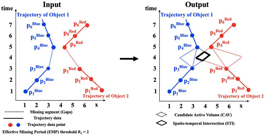
13:2   Analyzing Trajectory Gaps for Possible Rendezvous

       is shown in blue and Object 2 is shown in red. The gaps are shown in a dotted form and lie
       between P3, P4 for blue and P4, P5 for red. Object 1 has a maximum speed of 1 and Object
       2 has a maximum speed of 2. The output shows the candidate active volume (CAV) for each
       object. A CAV is the region in a gap that represents all the possible locations of the object
       during a missing time interval. The intersection of the two CAVs is the possible rendezvous
       region termed as a spatio-temporal intersection (STI).

          Figure 1 An illustration of rendezvous region detection (Best in color).

           Analysis of gaps in trajectories has many societal applications related to maritime safety,
       homeland security, epidemiology, and public safety. For example, maritime safety and
       regulation enforcement are important for global security for concerns such as illegal oil
       transfer and trans-shipments. Such activities can be restricted and managed by identifying
       frequent missing signals from GPS trajectories of oil vessels with gaps. However, the
       trajectories can be spread over a large geographical space and manual inspection for gaps
       to detect rendezvous can be time intensive. Computational methods that detect possible
       rendezvous regions can substantially reduce the preliminary work for human analysts.
           The problem is computationally challenging because the gaps may cause traditional
       trajectory mining approaches [27] to underperform or fail where they assume the availability
       and preciseness of trajectories. A second challenge is that the data has a large volume
       and is spread over considerable geographical space. For example, MarineCadastre [15] is
       an automatic identification system (AIS) dataset that contains records for more than 30
       attributes (e.g., location, draught) for 150,000 ships taken every minute during the years
       2009 to 2017. Its total size is about 600 GB and covers all the waters around the US.
           The literature on movement pattern analysis [2] and trajectory mining [27, 3] interpolates
       gaps in trajectories without considering the full range of an object’s movement possibilities.
       The approach provides an approximate solution and may miss possible rendezvous points.
       Areal interpolation of the gaps has been done through various prism models (e.g., space-time
       prism [16], kinetic prism [9]). Overlapping space-time prism for two or more objects can
       be thought of as a potential rendezvous region, or meeting place for moving objects. It
       may be computationally modeled as a spatio-temporal intersection of trajectories and can
       alternatively be called a spatio-temporal co-occurence.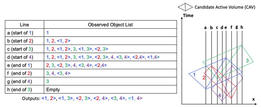
A. Sharma, X. Tang, J. Gupta, M. Farhadloo, and S. Shekhar                                        13:3

    In this paper, we study the computational cost of determining potential rendezvous
regions. The baseline method uses a plane sweep [18] technique to identify the potential
rendezvous regions. To improve the efficiency of plane sweep, we propose partitioning the
space into space-time grids. The grids are used to cover all the possible paths the object
can take. The grid overlapping two or more objects is a rendezvous region. The proposed
framework ensures completeness by finding all the possible rendezvous regions, and ensures
correctness because the rendezvous point is bound within the region. We further reduce
the geographical search space through time slicing techniques. We use plane-sweep as the
baseline to compare our results. Experimental results show that the proposed approach gives
tighter bounds. Further, results from time-slicing techniques improve as we increase the
time-slicing factor or use a finer time scale.

Contributions.
  We formally define the problem of rendezvous region detection for spatio-temporal
  trajectories with gaps.
  We propose a space-time partitioning approach to detect rendezvous regions. The approach
  is further refined to give more accurate approximation using time-slicing techniques.
  We propose and use a new evaluation metric, area pruning effectiveness (APE), to compare
  the methodologies.
  We compare the proposed approach with the plane sweep based baseline on various
  relevant evaluation parameters (e.g., study area) and metrics. Results (Section 4.2 show
  that the proposed approach has better APE values.
  We provide a case-study on ship trajectories from the Bering Sea to show the effectiveness
  of the proposed approach on a real-world dataset. We find that the proposed approach
  gives better results on the study area.

Scope. In this work, we do not study kinetic prisms [9]. Further, the proposed framework
has multiple phases and we limit this work to the filter phase. The refinement phase requires
input from a human analyst and is not addressed in this work. Furthermore, the calibration
of cost model parameters is outside the scope of this work. In addition, we do not model
rendezvous areas of trajectories without gaps which are involved in intersection. Finally, we
do not address the issue of positional accuracy while modeling the trajectories.

Organization. The paper is organized as follows: Section 2 introduces basic concepts and
the problem statement. Section 3 describes the proposed framework and approach used in
our work. Experiment design, results, and a brief discussion on the computation cost of
our approach are reported in Section 4. Section 5 reviews the related work (in more detail).
Finally, Section 6 concludes this work and briefly lists future work.

 2    Basic Concepts and Problem Statement

2.1    Basic Concepts
This section reviews several key concepts in the rendezvous detection problem and presents
a formal problem formulation.

I Definition 1. A study area is a two-dimensional rectangular area where the input data
are located. It usually complies with the (latitude, longitude) coordinate system.

                                                                                                GIScience 2021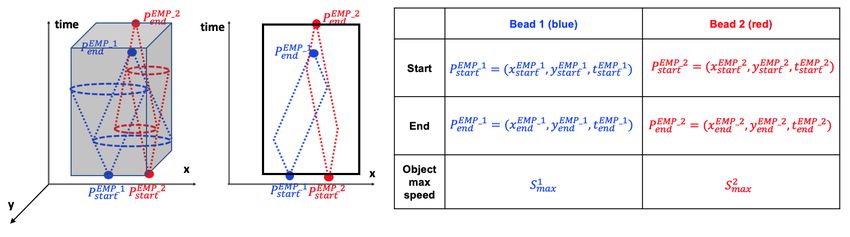
13:4   Analyzing Trajectory Gaps for Possible Rendezvous

       I Definition 2. A spatial trajectory is a trace generated by a moving object in a geographic
       space, that is usually interpreted as a series of chronologically sorted points, for instance,
       p1 → p2 → ··· → pn , where each point (pi ) is associated with a geospatial coordinate set
       (x, y) and a time stamp (t).

       I Definition 3. An object maximum speed (Smax) is the maximum speed of an object
       based on the domain knowledge.

       For maritime data, Smax can be identified from publicly available vessel databases [15]. For
       vehicles, humans, or animals, we can use the maximum physically allowed speed.

       I Definition 4. An effective missing period (EMP) is a time period when the signal is
       missing for longer than a user-specified EMP threshold (θe ) .

       As shown in Figure 1 the EMPs for Object 1 and Object 2 is between timestamps 3 and 4,
       Here, we assume θe = 2.

       I Definition 5. A candidate active volume (CAV) is the spatio-temporal volume where
       an object is possibly located during an EMP [4, 8, 11, 16, 17]. A CAV is based on a space
       time prism using conical shape and is derived from an EMP.

       2.2     Problem Formulation
       The problem to identify optimized rendezvous patterns in a spatio-temporal domain is
       formulated as follows:
          Input:
       1. A study area S,
       2. A set of |N | trajectories T = t1 . . . t|N | , each associated with an object,
       3. An object maximum speed (Smax ) for each object,
       4. An effective missing period threshold (θe ).

          Output: Approximate geometry intersection of two gaps.
          Constraints: Minimal Filter Storage Cost.
          Objective: Improve area pruning effectiveness (APE)
          For example, Figure 1 illustrates the one-dimensional representation of two gaps involving
       a spatiotemporal intersection given the study area (one-dimensional), two trajectories, two
       object maximum speeds, and θe = 2. The output is the STI represented by the triangle
       shown in the figure.
          Area pruning effectiveness (APE) is the ratio of the total study area and minimum
       bounded area inside the filtered region (i.e. approximate CAV).
                                                           total study area
            area pruning ef f ectiveness (AP E) =                                                (1)
                                                    area bounded inside the region
       If the value of AP E is higher, the solution quality is better since the minimum bounded area
       enclosed within a CAV will be lower.

        3      Approach
       We begin with an overview of our framework. Then we describe the baseline algorithm (plane
       sweep), a naive Spatio-temporal Grid Traversal (SGT), and the proposed Spatio-temporal
       Grid Traversal algorithm with time slicing (SGT-TS) in detail with their corresponding
       execution trace.
A. Sharma, X. Tang, J. Gupta, M. Farhadloo, and S. Shekhar 13:5
3.1 Framework
Our aim is to identify possible rendezvous regions on a given set of trajectories through
a two-phase Filter and Refine approach. Figure 2 shows a representation of the proposed
framework. The framework includes three algorithms: a baseline plane sweep algorithm
[18], a naive spatio-temporal grid (SGT) algorithm, and a spatio-temporal grid algorithm
with time slicing (SGT-TS). Plane sweep [18] is a basic computational geometry concept for
finding intersections (e.g., line segments, polygons). We used the plane sweep algorithm to
extract a minimum orthogonal bounding region (MOBR). SGT partition the study area into
3-dimensional (3D) grid cells (x,y, and time), where we approximate two endpoints based on
the maximum speed for each trajectory, and in total four endpoints including the starting,
and ending points of a gap segment that illustrates a possible rendezvous region. SGT-TS
adds a time-slicing technique for selecting a more accurate region that helps reduce data
redundancy and storage cost. The output from the filter phase is given to the refinement
phase where we can find the exact geometry of the cone intersect using accurate modeling
of the space-time prism of each object. The exact geometry can then be used by human
analysts for ground truth verification via satellite imagery.
Figure 2 Framework for detecting possible rendezvous regions to reduce manual inspection by
analyst.
3.2 Baseline Algorithm
Gaps in a trajectory can be analyzed by computing the minimum orthogonal bounding region
(MOBR) over the set of gaps for an individual trajectory. We use the plane sweep algorithm
[18] for extracting MOBRs. It is a filter and refine approach [5] where the given study area is
projected into a lower-dimensional space. In the filtering phase, all gaps are sorted based on
x or y coordinates. Ordering on one dimension reduces the storage and I/O cost, and further
allows the computation of intersections in a single pass. In the refinement phase, the gaps
are extracted based on the start and end times of their respective effective missing periods
(EMPs). The segments are further approximated using MOBRs over each candidate active
volume (CAV). The following text describes the algorithm in detail.
Step 1: Sort the endpoints of all the effective missing periods (EMPs). First, we sort
the endpoints of all EMPs based on one of the coordinates. An endpoint is represented by
three coordinates, namely x, y, and time, and either x or y can be the sorting coordinate.
For consistency, we use x throughout this paper.
GIScience 202113:6 Analyzing Trajectory Gaps for Possible Rendezvous
Step 2: A plane orthogonal to the x-axis sweeps along the sorted EMPs. The second
step conducts the sweeping. Imagine there is a plane parallel to the y-t plane and orthogonal
to the x-axis sweeping from the low to the high end along x-axis. The sweeping plane stops
at both start and end points of each EMP. Note that “start” and “end” refer to the order
of sweeping, which is irrelevant to the temporal dimension. An Observed Object List is
maintained to store CAVs being currently crossed by the sweeping plane.
When stopping at the start of an EMP, the algorithm first determines if the gap is larger
than the given EMP threshold (θe ). If it is, a new CAV is constructed for that object along
with an approximate MOBR around the new CAV as discussed later in Section 3.3. The
CAV along with its MOBR is then saved inside the observed list and a check is done to see if
any other CAV inside the list is intersecting with the given CAV. If it is, a common MOBR
around the pair of intersecting CAVs is added to the observed list as well as the output.
The sufficient and necessary condition for the spatiotemporal intersection of two CAVs is
explained in 3.3. On the other hand, when stopping at the end of an EMP, the algorithm
removes all the STIs that involve the EMP from the list. Note that each of these CAVs has
different corresponding time periods indicating when the possible rendezvous may happen.
We introduce how to compute the time period in the following Section 3.3.
Figure 3 Plane sweep execution trace with a test case.
An execution trace of Plane Sweep. Figure 3 shows a dataset containing EMPs and their
corresponding CAVs from four objects. For illustration, we simplify the study area into
one-dimensional geographical space. A vertical line sweeps from left to right and stops at
the endpoints (from a to h) of each EMP. The table on the left shows the elements in the
observed object list after each stop. For example, when stopping at Line d (start of 4), the
algorithm determines whether the incoming EMP < 4 > intersects with any element in the
observed object list, namely < 1 >, < 2 >, and < 3 >. Hence, < 1, 4 >, < 2, 4 > and
< 3, 4 > are added to the observed list and the output list. When stopping at Line e (end of
1), the algorithm removes all the elements in the list involving EMP < 1 > which includes
< 1, 2 >, < 1, 3 >, and < 1, 4 >. The last stop is at Line h (end of 3). The Observed Object
List becomes empty and the final output STIs include: < 1, 2 >, < 1, 3 >, < 2, 3 >, < 2, 4 >,
< 3, 4 >, and < 1, 4 >.A. Sharma, X. Tang, J. Gupta, M. Farhadloo, and S. Shekhar 13:7
3.3 Constructing a Minimum Orthogonal Bounding Region and
Spatiotemporal Intersection
In section 3.2, we explained the intuition behind the baseline algorithm along with its
corresponding execution trace. Now we explain in more detail the creation of candidate
active volumes(CAVs) and new minimum orthogonal bounding regions (MOBRs). A loop
goes over all the EMPs with gaps and checks if the given EMP is greater than the missing
threshold. If it is, then a new CAV is constructed bounded by the coordinates attained
through maximum speed and a check is done to see if any other CAV in the observed list
intersects with the new given CAV. If it does, a new common MOBR is constructed around
the intersection of the two CAVs using their maximum and minimum coordinates. The
sufficient and necessary condition of whether two CAVs intersect is discussed later in this
section.
Figure 4 Cone Intersection of Effective Missing Period (EMPs).
As defined in Section 3.2, an effective missing period (EMP) is the intersection of two
cones (i.e., a bead) vertexed at the endpoints of a CAV [26]. Therefore, in order to construct
a new CAV during each iteration of this loop, we first need to determine the coordinates of
the end points attained via maximum speed along with their respective radius. As shown
in Figure 4, we first construct a CAV using maximum speed and radius where the radius
of each cone at time t is the product of the object max speed Smax and the time difference
EM P1
from the start point of the EMP. For example, the radius of the cone vertexed at PEnd at
P1 P2 1
time t: rend = (tend − t) × Smax . Then, we find the end points by calculating the distance
covered at maximum speed from each start point to its respective end point. This operation
is done for both CAVs and creates a common MOBR using the extreme coordinates bounded
by each CAV.
To compute the intersection between two EMPs during each iteration of this loop, we
need to determine the intersections between four cones (i.e. two beads). We first check
whether two beads have an overlapping time range. If not, then the beads are guaranteed
to be not intersecting. Otherwise, the following geometric property is used to determine
the intersection. Figure 4 shows two beads generated from two EMPs. EM P1 starts at
EM P1 EM P1 EM P2 EM P2
Pstart and ends at Pend , while EM P2 starts at Pstart and ends at Pend . Each point is
EM P1 EM P1 EM P1 EM P1
represented by three coordinates. For example, start point Pstart = (xstart , ystart , tstart )
EM P1 EM P1
is presented by two spatial coordinates xstart and ystart as well as the temporal coordinate
tEM P1
start . The radius of each cone at time t is the product of the object max speed Smax and
the time difference from the start point of the EMP. For example, the radius of the cone
EM P1 EM P1
vertexed at Pend at time t: rend = (tEM
end
P1 1
− t) × Smax . Now, we formulate the sufficient
and necessary condition for two beads intersect as follows:
rstart + rend ≤ dis(start, end), (2)
GIScience 202113:8 Analyzing Trajectory Gaps for Possible Rendezvous
where index start = {startEM P1 , startEM P2 }, index end = {endEM P1 , endEM P2 }, and
disstart,end is the Euclidean distance between points Pstart and Pend . Appendex A includes
a detailed proof for Equation 2.
3.4 Spatio-temporal Grid Traversal Algorithm
Computing possible rendezvous regions is challenging due to the high computational cost
over a large set of trajectories as discussed in Section 1. The plane sweep algorithm provides
an axis parallel MOBR which reduces the search space for finding the possible rendezvous
regions for the refinement phase. However, this baseline approach proves to be inefficient
when pruning a set of gap pairs both having higher positional displacement and EMPs. This
may result in the construction of a common MOBR with size similar to the entire study area
even if the actual rendezvous region between the gap pairs is relatively small compared to
their respective MOBRs. Thus, we propose a spatio-temporal grid traversal algorithm (SGT)
that aims to identify possible rendezvous regions using location, time and maximum speed.
Spatio-temporal grid traversal (SGT) is based on the idea of a 3D filtering technique
by leveraging spatiotemporal properties and additional attributes of the space-time prism
model to get a better geometric approximation of a bounded region. SGT starts by creating
a spatiotemporal grid and applying the baseline approach for constructing CAVs of incoming
gaps followed by the a common minimum object bounded rectangle (MOBR). However, inside
each MOBR, we compute the linear bounds of the cones generated from the start and end
point of the individual gaps and determine which grid cells reside inside the linear bounds
of each CAV by checking each of the cell’s corner points. Then we check the common cells
residing in both CAVs. This operation is performed for every slice in the third dimension.
Algorithm 1 shows the pseudo-code for SGT.
Step 1: Create common minimum orthogonal bounding rectangles (MOBRs). First, we
create a spatio-temporal grid having the size of the given study area and a specified spatial
and temporal resolution. Then, we apply the plane sweep algorithm to get common MOBR
around gap pairs as described in Section 3.3 and save them in a common MOBR list.
Step 2: Create linear bounds within each common MOBR. For each common MOBR
inside the common MOBR list, we index its endpoints inside the spatio-temporal grid along
with the start and end points of the individual gaps to their respective nearest cell. Next
we derive CAV linear bounds from the start point and end point of each gap based on the
object’s maximum speed. The linear bounds can be defined as the geometric interpretation
of the slant height of the cone derived from the object’s maximum speed. The maximum
speed provides the slope i.e. the angle between the slant height and the time axis.
Step 3: Filter remaining grid cells qualified within CAVs. The filtering step linearly checks
whether each cell inside the MOBR resides in the given CAV linear bounds. The linear
bounds can be further divided into lower bounds and the upper bounds which can be derived
from the start and end points of the gap respectively using object’s maximum speed. In order
to satisfy this condition, at least one of the corner points should be positioned higher than
the lower bound but lower than the upper bound for each individual CAV. During filtering,
we further refine the intersection by concurrently checking if any of those cells reside in both
the CAVs. If they do, we filter out the remaining cells into the output list.A. Sharma, X. Tang, J. Gupta, M. Farhadloo, and S. Shekhar 13:9
Algorithm 1 Spatio-temporal Grid Traversal (SGT).
1: Spatial Resolution ← M
2: T emporal Resolution ← T
3: Create Spatiotemporal Grid
4: CM OBR list ← ∅
5: Output ← ∅
6: Apply Plane Sweep Algorithm for Commom MOBRs
7: CM OBR list ← Common M OBRs
8: for each: CM OBRi in CM OBR list do
9: Index CM OBRi over Spatial T emporal Grid
10: Calculate Linear Bounds of CAV s
11: for each: Celli inside Common M OBR do
12: if Celli resides in
both CAV s then
13: Celli → Output
14: end if
15: end for
16: end for
Time Slicing. Time slicing is an intermediate filtering phase which bounds each cone slice
by a rectangle which is tighter than the corresponding slice of the space-time grid, thereby
achieving higher efficiency. Hence, increasing the number of slices greater than the spatial
resolution extent results in finer pruning that filters out any extra space between the CAV
bounds and MOBR. Algorithm 2 provides a modification of step 2 in Algorithm 1 where we
increase the temporal resolution greater than its respective spatial resolution.
Algorithm 2 Spatio-temporal Grid Traversal with Time Slicing (SGT-TS).
1: Spatial Resolution ← M
2: T emporalResolution ← t > T
3: Run Algorithm 1 (line: 3 to 16)
Execution trace of SGT and SGT-TS. Figure 5 shows the execution trace of Algorithms
1 and 2 over a 2D grid with 64 cells taking the x-axis as longitude (or latitude) and the y
axis as time. For a given pair of CAVs, we first create a common MOBR and approximate
its end points to their respective nearest cells. Figure 5(a) shows a 16x4 example grid with a
CAV surrounded by its MOBR approximated by a grid where each grid cell is marked in
yellow. During the filtering phase, SGT checks whether the corners of each cell qualify to be
included in the given CAV. Figure 5 (b) shows the resulting grid after filtering where cells
marked in red do not qualify and yellow cells represent the cells residing in the CAV. After
getting all the cells inside the MOBRs, we check whether each remaining cell (yellow) resides
in both the CAV pairs and output them as the final output. Figure 5 (c) shows the blue
cells which take part in the intersection of two CAVs. For SGT with time slicing, we increase
in temporal resolution providing a better filter as compared to the original SGT. Figure 5
(d) shows the final grid cells remaining in yellow and discarded cells in red. As compared to
SGT, SGT-TS gives more refined results since more extra space has been discarded. Figure 5
(e) shows a greater number of intersecting cells, represented in blue, and indicating a better
approximation of the intersection area.
GIScience 202113:10 Analyzing Trajectory Gaps for Possible Rendezvous
Figure 5 Execution Trace of SGT and SGT-ST.
4 Validation
In this section, we validated our approach using real world data in a case study as well as
experimentally by varying different parameters such as study area and number of objects.
4.1 Experiment Design
Dataset. The dataset used in the experiments was MarineCadastre [15] which contains
records of more than 30 attributes (e.g., Maritime Mobile Service Identity (MMSI), longitude,
latitude, speed over ground (SOG), course over ground (COG) etc.) for 150,000 objects
(i.e. ships) taken every minute from 2009 to 2017. The dataset is based on the WGS 1984
coordinates system with a geographical extent of 180W to 66W degrees in longitude and 90S
to 90N degrees in latitude covering waters around the US.
Experimental goal. The goal was to evaluate the performance of the proposed baseline,
SGT and SGT-TS under different parameters. Our research questions are as follows:
(1) How does the size of the study area affect the APE ? and (2) How does an increase in
the number of objects affect the APE on a given study area ?
Our evaluation metric was area pruning effectiveness (APE) which is the ratio of the total
study area and minimum bounded area inside the filtered region (i.e. approximate CAV) as
discussed in Section 2.2.
Computing Resources. All the experiments were conducted using Python and performed
on an Intel Core i5 2.5GHz CPU and 16GB memory.
4.2 Experimental Results
Effect of the size of study area. In this experiment, we tested three study area sizes:
2000km2 , 4000km2 and 8000km2 . The number of GPS points varied for each study area as
1.5×10⁵ , 3×10⁵ , and 6×10⁵ . The density of GPS points remained consistent for the different
areas. The results in Figure 6a show that SGT and SGT-TS are always more accurate than
the baseline, especially as the study area increases. Figure 6b shows the APE values for
SGT-TS with increasing time-slicing factor. Again, the SGT-TS algorithm outperforms the
baseline with the APE improving as the time-slicing factor is increased.
Effect of the number of objects. In this experiment, we set the study area size to 8000km2
and varied the number of object pairs (i.e. ships) from 500 to 2, 000. We also varied the
number of GPS points respectively from 2.5 × 10⁴ to 4.5 × 10⁴ . This was realized by pickingA. Sharma, X. Tang, J. Gupta, M. Farhadloo, and S. Shekhar 13:11
(a) Comparison based on Study Area.
(b) Change in Time Slicing (8000 km2 ).
(c) Comparison based on Object number. (d) Change in Time Slicing (300 obj.).
Figure 6 Effects on area pruning effectiveness (APE).
same study area from the original dataset for each varied number of object pairs resulting in
different density of GPS points. The results in Figure 6c show that the increase in average
pruning effectiveness (AP E) is significantly greater in SGT and SGT-TS as compared to
plane sweep for different number of objects. Figure 6d shows the further improvement of the
AP E as we increase the time-slicing factor.
4.3 Interpretation of Experimental Results
Scanning an entire study area can be exponentially expensive in terms of computational cost
and human effort. The filter phase provides approximate regions within a trajectory gap for
filtering possible rendezvous regions. However, the refinement phase can be expensive due to
uncertainty in modeling the exact geometry of cones. Exact geometry involves inclusion of
many real world physics based parameters (e.g. speed, acceleration) [9] which add complexity
due to the need to solve quadratic equations. Hence, our main intuition is to reduce the total
refinement cost in terms of computation of each cell per unit area by providing a tighter and
GIScience 202113:12 Analyzing Trajectory Gaps for Possible Rendezvous
more accurate filter in the filtering phase. Equation 3 shows the relationship of filter and
refinement in terms of computational cost.
Cf + Cr = Ct , (3)
where Cf is the cost of filtering, Cr is the cost of refinement and Ct is the total cost to
prune the given study area. The cost of refinement Cr decreases as we increase the filtering
efficiency which often requires high computational cost in terms of prepossessing, model
refinement, etc. However, if we are not considering any filtering then Cr will be equal to Ct .
4.4 Case Study on Real Automatic Identification System (AIS) data
We conducted a case study on data from MarineCadastre, a popular real world AIS dataset [15]
to find possible rendezvous regions using the algorithms proposed in the paper. The
approaches were applied on a study area ranging from 179.9W to 171W degrees in longitude
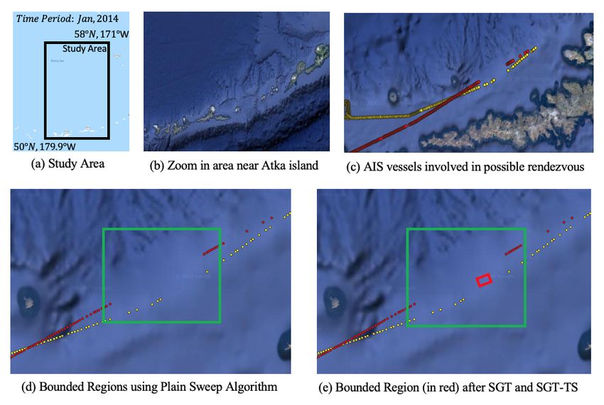
and from 50N to 58N degrees in latitude in the Bering Sea, shown in Figure 7 (a). The
dataset contained ~1.4 × 10⁶ GPS readings from 72 ships that traveled during January, 2014.
The EMP threshold (θe ) was set to 30 minutes by which only the top 0.5% longest missing
periods were considered as EMPs. We focused on various different trajectories that formed
two STI clusters, one near Idak, and Atka Islands. These clusters accord with reports by the
Marine Traffic Agency [24] that near an island, AIS systems tend to switch back and forth
between terrestrial-AIS and satellite-AIS. Ships moving across the boundary of the effective
zone may put out weak and unstable signals. The STI clusters we identified, which are near
islands, likely represent such areas of weak signaling. Figure 7 (b) shows the zoomed in
region near Atka Island where we selected to study our case. Figure 7 (c) shows the voyage
of two vessels in that region categorized by a unique identifier (MMSI) each represented
by a unique color indicating the start and end points of the EMPs. Figure 7(d) shows the
output of the plane sweep algorithm, which construct a common MOBR around the CAV’s
(in green). Figure 7 (e) shows the common region (shown in red) after applying SGT and
SGT-TS inside the MOBR where both the CAVs intersect, providing a significantly smaller
region and better area effective pruning (APE) than the baseline approach.
5 Related Work and Limitations
Due to recent advancements in location-acquisition services, and mobile computing research,
an extensive amount of trajectory data is available which serve different research purposes such
as pattern recognition, anomaly detection, etc. The work in [27] provides a comprehensive
survey of trajectory data mining and also explores the connection between different research
topics and existing methodologies. Reconstruction techniques in [27] illustrate a variety of
frameworks for modeling uncertainty and noise in trajectory data. However, all the techniques
are based on assumptions related to linear interpolation or shortest path discovery. These
approaches are not designed to detect patterns when the trajectories of the moving objects
are missing (e.g., due to weak signaling) in which case the objects possibly move far from
the shortest path. Trajectory data mining has also motivated interdisciplinary research in
other fields such as geography and ecology. In [2], the authors provide a unified taxonomy
of moving objects concerning their movement patterns by classifying them into generic and
behavioral patterns, which encompass patterns such as co-locations, co-occurrence, etc.
Movement behavior patterns such as evasive patterns are used to detect potential anom-
alies. Analyzing maritime trajectory data with gaps is a particular case of an evasive pattern.
A recent survey, [21] provides a panorama of existing techniques to identify anomalousA. Sharma, X. Tang, J. Gupta, M. Farhadloo, and S. Shekhar 13:13
Figure 7 Spatio-temporal intersections detected in Bering Sea (best in color). The background
imagery is not taken at the same time when the vessels were traveling in January 2014.
patterns in maritime trajectories by classifying them as data-driven, signature-based, and
hybrid methods. Many frameworks [12, 1, 23, 13] have been proposed for analyzing evasive
patterns in maritime trajectories. For instance, the authors in [13] proposed a method for
determining if the vessel is anomalous by considering longitude, latitude, speed, and direction
for each trajectory point and providing a three-division distance that can detect anomalous
navigational behaviors. Stop and move [25] is an another conceptual model which analyzes
anomalous behavior based on DBSCAN [19], and speed and direction [22], when it comes
to ship trajectories data. These techniques do not apply to our work, which is focused on
interpreting gaps in trajectory data, rather than detecting anomalous behaviour.
More realistic solutions for modeling gaps in trajectory data are contextual models
such as space-time prisms [16, 6] that construct an areal interpolation of the gaps using
coordinates and maximum speed of the objects. More recently, the kinetic prism model [9]
provides a better estimation by considering other physical parameters such as uncertainty
and acceleration. However, applying these models can be computationally expensive. One
way to address the cost is through spatial indexing. Many spatial indexing techniques such
as 3D R-Trees [28] or many others as described in [28], [20], [14] could be used to index
trajectories efficiently. Other spatial indexing techniques, such as Hilbert Curve [20] have
also been used to provide a computational speedup. The literature related to space-time
prisms addresses computational speedup by using an alibi query for checking whether two
space-time prisms intersect theoretically [10] which have also been applied in road networks
[7]. In this work, we introduce the use of space-time prisms with grid-based indexing for
detecting possible rendezvous patterns over maritime trajectories.
GIScience 202113:14 Analyzing Trajectory Gaps for Possible Rendezvous
6 Conclusion and Future Work
In this paper, we introduced the problem of rendezvous detection in trajectory data with gaps.
We proposed a baseline algorithm based on a plane sweep approach which first sorts and does
a linear scan over a set of gaps and then provides a minimum orthogonal bounding region
around the gaps. We proposed a spatio-temporal grid traversal (SGT) that provides tighter
MOBRs, which in turn provides a more approximate shape of the candidate active volumes
(CAVs). We further add efficient pruning based on time-slicing (SGT-TS) by adding a finer
temporal resolution that gives a more accurate approximation bounded by the intersection
of two cones. The results show relatively better area density ratio in SGT with time slicing
(SGT-TS) as compared to SGT with significantly better AP E when compared to the baseline.
Future Work. We plan to further implement the refinement phase where we refine the
process of finding the exact geometry of spatiotemporal intersection since it is hard to find
the exact geometry of the cone intersect due to its complexity. Computing approximate
regions is very expensive in terms of time complexity and modeling them in regional space
is challenging. Hence, we plan to further address the computational cost for extracting
gaps and extend the proposed work in regional space as described in [10] [7]. We will also
study if there an empirical threshold or ratio beyond which the gap may be too large to be
meaningfully estimated via space-time prism. In addition, we will create synthetic dataset
and then remove data points to make the data coarse for evaluating precision and recall with
known rendezvous regions. Finally, we will analyze more interesting rendezvous patterns
which involve more than two objects where the intersection of multiple space-time prisms
takes place.
References
1 Elena Camossi, Paola Villa, and Luca Mazzola. Semantic-based anomalous pattern discovery
in moving object trajectories. arXiv preprint arXiv:1305.1946, 2013.
2 Somayeh Dodge, Robert Weibel, and Anna-Katharina Lautenschütz. Towards a taxonomy of
movement patterns. Information visualization, 7(3-4):240–252, 2008.
3 Emre Eftelioglu, Xun Tang, and Shashi Shekhar. Avoidance region discovery: A summary of
results. In Proceedings of the 2018 SIAM International Conference on Data Mining, pages
585–593. SIAM, 2018.
4 Kathleen Hornsby and Max J Egenhofer. Modeling moving objects over multiple granularities.
Annals of Mathematics and Artificial Intelligence, 36(1-2):177–194, 2002.
5 Edwin H Jacox and Hanan Samet. Spatial join techniques. ACM Transactions on Database
Systems (TODS), 32(1):7–es, 2007.
6 Hyun-Mi Kim and Mei-Po Kwan. Space-time accessibility measures: A geocomputational
algorithm with a focus on the feasible opportunity set and possible activity duration. Journal
of geographical Systems, 5(1):71–91, 2003.
7 Bart Kuijpers, Rafael Grimson, and Walied Othman. An analytic solution to the alibi query
in the space–time prisms model for moving object data. International Journal of Geographical
Information Science, 25(2):293–322, 2011.
8 Bart Kuijpers, Harvey J Miller, Tijs Neutens, and Walied Othman. Anchor uncertainty
and space-time prisms on road networks. International Journal of Geographical Information
Science, 24(8):1223–1248, 2010.
9 Bart Kuijpers, Harvey J Miller, and Walied Othman. Kinetic prisms: incorporating acceleration
limits into space–time prisms. International Journal of Geographical Information Science,
31(11):2164–2194, 2017.A. Sharma, X. Tang, J. Gupta, M. Farhadloo, and S. Shekhar 13:15
10 Bart Kuijpers and Walied Othman. Modeling uncertainty of moving objects on road networks
via space–time prisms. International Journal of Geographical Information Science, 23(9):1095–
1117, 2009.
11 Mei-Po Kwan. Gis methods in time-geographic research: Geocomputation and geovisualization
of human activity patterns. Geografiska Annaler: Series B, Human Geography, 86(4):267–280,
2004.
12 Po-Ruey Lei. A framework for anomaly detection in maritime trajectory behavior. Knowledge
and Information Systems, 47(1):189–214, 2016.
13 Bo Liu, Erico N de Souza, Cassey Hilliard, and Stan Matwin. Ship movement anomaly
detection using specialized distance measures. In 2015 18th International Conference on
Information Fusion (Fusion), pages 1113–1120. IEEE, 2015.
14 Ahmed R Mahmood, Walid G Aref, Ahmed M Aly, and Saleh Basalamah. Indexing recent
trajectories of moving objects. In Proceedings of the 22nd ACM SIGSPATIAL International
Conference on Advances in Geographic Information Systems, pages 393–396, 2014.
15 Marinecadastre.gov. URL: https://marinecadastre.gov/ais/.
16 Harvey J Miller. Modelling accessibility using space-time prism concepts within geographical
information systems. International Journal of Geographical Information System, 5(3):287–301,
1991.
17 Tijs Neutens, Tim Schwanen, and Frank Witlox. The prism of everyday life: Towards a new
research agenda for time geography. Transport reviews, 31(1):25–47, 2011.
18 Jürg Nievergelt and Franco P. Preparata. Plane-sweep algorithms for intersecting geometric
figures. Communications of the ACM, 25(10):739–747, 1982.
19 Andrey Tietbohl Palma, Vania Bogorny, Bart Kuijpers, and Luis Otavio Alvares. A clustering-
based approach for discovering interesting places in trajectories. In Proceedings of the 2008
ACM symposium on Applied computing, pages 863–868, 2008.
20 Dieter Pfoser, Christian S Jensen, Yannis Theodoridis, et al. Novel approaches to the indexing
of moving object trajectories. In VLDB, pages 395–406, 2000.
21 Maria Riveiro, Giuliana Pallotta, and Michele Vespe. Maritime anomaly detection: A review.
Wiley Interdisciplinary Reviews: Data Mining and Knowledge Discovery, 8(5):e1266, 2018.
22 Jose Antonio MR Rocha, Valéria C Times, Gabriel Oliveira, Luis O Alvares, and Vania
Bogorny. Db-smot: A direction-based spatio-temporal clustering method. In 2010 5th IEEE
international conference intelligent systems, pages 114–119. IEEE, 2010.
23 Hamed Yaghoubi Shahir, Uwe Glässer, Narek Nalbandyan, and Hans Wehn. Maritime situation
analysis: A multi-vessel interaction and anomaly detection framework. In 2014 IEEE Joint
Intelligence and Security Informatics Conference, pages 192–199. IEEE, 2014.
24 Katerina Sofrona. Why cannot i see a vessel on the live map?, October 2017. URL: https:
//help.marinetraffic.com/hc/en-us/articles/203990958.
25 Stefano Spaccapietra, Christine Parent, Maria Luisa Damiani, Jose Antonio de Macedo,
Fabio Porto, and Christelle Vangenot. A conceptual view on trajectories. Data & knowledge
engineering, 65(1):126–146, 2008.
26 Goce Trajcevski, Alok Choudhary, Ouri Wolfson, Li Ye, and Gang Li. Uncertain range queries
for necklaces. In 2010 Eleventh International Conference on Mobile Data Management, pages
199–208. IEEE, 2010.
27 Yu Zheng. Trajectory data mining: an overview. ACM Transactions on Intelligent Systems
and Technology (TIST), 6(3):1–41, 2015.
28 Qing Zhu, Jun Gong, and Yeting Zhang. An efficient 3d r-tree spatial index method for
virtual geographic environments. ISPRS Journal of Photogrammetry and Remote Sensing,
62(3):217–224, 2007.
GIScience 202113:16 Analyzing Trajectory Gaps for Possible Rendezvous
A Necessary and Sufficient Condition of Spatiotemporal Intersection
Lemma. Two beads must be intersected if and only if
rstart + rend ≤ dis(start, end) (4)
where index start = {startEM P1 , startEM P2 }, index end = {endEM P1 , endEM P2 }, and
disstart, end is the Euclidean distance between points Pstart and Pend .
Proof. For the necessary condition there must be at least one timestamp when the sections
of these two beads intersect i.e. if two beads have an overlapping time range, at least one-time
stamp (start-point or the end point) of one of the gap segments must be between the time
range of the other. To prove this, we take two data gaps, EM P1 and EM P2 having time
range (t1start , t1end ) and (t2start , t2end ) respectively and check if the difference between (t1start ,
t2end ) or (t1end , t2start ) ≥ 0. If true, then the two EMPs satisfy the necessary condition of a
two EMP intersect.
For the sufficient condition, if there is one timestamp that is between the overlap of the
time gaps, the two beads must intersect. In order to satisfy this condition, we use the radius
information of two cones from a different gap and check whether their respective radii will
overlap with each other. According to the condition whether two circles overlap, the sum of
their radii must be smaller than the distance between their respective centers. As stated
1
in Equation 4, the sum of the radius of the cone from start point rstart of EM P1 and end
2
point rend of EM P2 must be less than the distance between their respective radii centers
1 2
dist(s, e). Using known t and Smax , when Smax ≥ Smax , Equation 4 is further derived into:
1 2
ds,e + ts × Smax + te × Smax
t≥ 1 2
→ where s = startEM P1 , e = startEM P2 (5)
Smax + Smax
1 2
ds,e + ts × Smax − te × Smax
t≥ 1 2
→ where s = startEM P1 , e = endEM P2 (6)
Smax − Smax
2 1
ds,e + ts × Smax − te × Smax
t≤ 2 1
→ where s = endEM P1 , e = startEM P2 (7)
Smax − Smax
1 2
ds,e + ts × Smax − te × Smax
t≤ 1 2
→ where s = endEM P1 , e = endEM P2 (8)
−Smax − Smax
1 2
In the case that Smax < Smax , the conditions are derived by swapping the variables.
If the conditions are all satisfied, we know these two EMPs intersect. In contrast, if any of
the conditions is not satisfied, the two EMPs do not intersect.You can also read