Connectivity domain analysis: characterization of connectivity frequency profile using filter banks - bioRxiv
←
→
Page content transcription
If your browser does not render page correctly, please read the page content below

bioRxiv preprint first posted online Jul. 18, 2019; doi: http://dx.doi.org/10.1101/706838. The copyright holder for this preprint (which
 was not peer-reviewed) is the author/funder, who has granted bioRxiv a license to display the preprint in perpetuity.
 All rights reserved. No reuse allowed without permission.

 Connectivity domain analysis: characterization of connectivity
 frequency profile using filter banks
 Ashkan Faghiria,b, Armin Irajia, Eswar Damarajua, Jessica Turnerc, Vince D.
 Calhouna,b,c
 a
 The Tri-institutional Center for Translational Research in Neuroimaging and Data Science, [Georgia State University Georgia Institute of
 Technology, Emory], Atlanta, GA, USA
 b
 School of Electrical and Computer Engineering, Georgia Institute of Technology, Atlanta, GA 30302, USA
 c
 Department of Psychology, Georgia State University, GA, USA
 Abstract
 Studying functional network connectivity using different imaging modalities has been the focus of many
 studies in recent years. One category of methods assumes that the connectivity is constant throughout
 the whole scanning period (e.g. using Pearson correlation to estimate linear correlation between two time
 series each belonging to a specific region in brain) while others relax this assumption by estimating
 connectivity at different time scales. The most common way to estimate dynamic functional network
 connectivity (dFNC) uses sliding window in combination with a connectivity estimator such as Pearson
 correlation (SWPC). The estimated values resulting from this method are effectively subjected to a low-
 pass filter (due to the sliding window) which can result in loss of connectivity information for high
 frequencies.

 Here, we propose a new approach to estimate connectivity while preserving its full frequency range using
 filter banks for frequency tiling in the connectivity domain directly. This is in contrast with many other
 methods where frequency tiling is performed in the activity domain and indirect inferences are made
 about the connectivity frequency profile. Using our approach, we can estimate the full connectivity
 spectrum and subsequently examine both static and dynamic connectivity changes in one unified
 approach. In addition, the filter length (i.e. window length in SWPC) has minimal effect on the results of
 our approach as we are able to design our filters to have any desired band-pass range regardless of the
 length of filter. This method is called filter banked connectivity (FBC).

 After demonstrating the approach on a simulated dataset, we use the FBC approach to estimate dFNC in
 a resting fMRI data set including schizophrenia patients (SZ, n=151) and healthy controls (HC, n=163). To
 summarize the results, we used k-means to cluster the FBC values into different clusters and calculate the
 total amount of time each subject spends in each cluster. These values are then compared between HC
 and SZ across different frequency bands. Using FBC we observed two states with very low frequency
 profiles where SZ patients tend to stay more in one of these states while HCs tend to stay more in the
 other states. In addition to common states found using SWPC, we were able to find some additional states
 not previously identified. These states showed very weak low frequency strength and as such SWPC was
 not well suited to capture them. In summary, the proposed approach offers a more comprehensive way
 to analyze connectivity (including both static and dynamic values).

 Introduction
bioRxiv preprint first posted online Jul. 18, 2019; doi: http://dx.doi.org/10.1101/706838. The copyright holder for this preprint (which
 was not peer-reviewed) is the author/funder, who has granted bioRxiv a license to display the preprint in perpetuity.
 All rights reserved. No reuse allowed without permission.

 Functional network connectivity (FNC; which estimated dependence between coherent networks typically
 estimated with independent component analysis) have been the focus of many neuroimaging studies over
 the past few decades. We can group these methods into two major categories: those that assume
 connectivity among different networks of the brains is constant through time (static FNC; sFNC) and those
 that assume temporal variation in connectivity (dynamic FNC; dFNC). Both sFNC and dFNC have proven to
 be extremely informative about both healthy and diseased brain function and can be used to study
 different neuroimaging modalities, including functional magnetic resonance imaging (fMRI).

 dFNC estimation approaches

 While sFNC has resulted in many interesting findings (Di Martino et al., 2008; van den Heuvel and Hulshoff
 Pol, 2010), this view of FNC is limited to the average connectivity patterns over the entire experiment.
 Approaches designed based on the dFNC idea relax the assumption of static connectivity. The most
 common way to estimate dFNC uses a sliding window to estimate time-varying connectivity. Typically
 sliding window is paired with Pearson correlation (SWPC) (Allen et al., 2014; Faghiri et al., 2018; Hutchison
 et al., 2013b; Kucyi and Davis, 2014). Using a sliding window to estimate dFNC has the benefit of being
 straightforward but it has two major shortcomings. First to use a sliding window we need to choose a
 window size. We want to choose a window size that is large enough so that the standard error is as small
 as possible while it should be small enough to allow us to detect faster changes in dFNC (Hutchison et al.,
 2013a). The second shortcoming of the sliding window approach is its low-pass nature (Leonardi and Van
 De Ville, 2015; Sakoglu et al., 2010; Thompson and Fransson, 2015). Regardless of which window size is
 chosen, the estimated dFNC is subjected to a low-pass filter and therefore we do not capture the full
 frequency range of dFNC.

 Another category of methods that aim to explore the frequency profile of connectivities use time-
 frequency analysis ideas. The most well-known methods in this category use wavelet (Mallat, 1999). While
 these methods have resulted in many interesting findings in fMRI (Chang and Glover, 2010; Yaesoubi et
 al., 2015; Yaesoubi et al., 2017), these studies have several limitations. Firstly, the interpretation of the
 results in these studies can be challenging. The Chang and Glover implementation of wavelet resulted in
 a huge amount of information without ways to succinctly summarize the results (Chang and Glover, 2010).
 To remedy this, Yaesoubi et al. proposed an approach using wavelets that can be used to study group
 differences, but their results are all in the wavelet domain (Yaesoubi et al., 2015). This presents a difficulty
 in connecting the reported results to other studies on dFNC as most dFNC studies work in the time domain
 (the time domain results are typically considered easier to interpret).

 In addition, both wavelet approaches perform frequency tiling in the activity domain instead of the
 connectivity domain. We believe that to discuss the frequency properties of dFNC it is important to
 implement all time-frequency tiling steps directly in the connectivity domain, as the relationship between
 activity and connectivity domain is a unknown (possibly non-linear) and therefore the frequency
 information is distorted when transforming from activity to connectivity domain.

 Apart from the two categories of approaches mentioned above, other methods have been proposed to
 estimate dFNC in past years. Some of these methods are hidden Markov models (Ou et al., 2013),

bioRxiv preprint first posted online Jul. 18, 2019; doi: http://dx.doi.org/10.1101/706838. The copyright holder for this preprint (which
 was not peer-reviewed) is the author/funder, who has granted bioRxiv a license to display the preprint in perpetuity.
 All rights reserved. No reuse allowed without permission.

 coactivation patterns using clustering approaches (Liu and Duyn, 2013) and window-less dictionary
 learning approaches (Yaesoubi et al., 2018).

 Schizophrenia-related findings

 There have been a number of studies of functional connectivity in schizophrenia using resting fMRI. For
 example, Camchong et.al. reported hyperconnectivity between default mode network (DMN) and the rest
 of the brain (Camchong et al., 2011). In another work, (Jafri et al., 2008) used a whole brain approach to
 study the differences between healthy controls (HC) and individuals with schizophrenia (SZ). They
 reported that SZ showed increase connectivity between DMN and visual and frontal functional domains
 compared to HC. Damaraju et al., reported that SZ compared to HC show increased connectivity between
 thalamus and sensory functional domains (Damaraju et al., 2014). Damaraju et al., also reported
 decreased static connectivity in sensory domains when comparing SZ to HC. Decrease connectivity in SZ
 compared to HC has been reported in other studies too (Erdeniz et al., 2017; Skudlarski et al., 2010). A
 few studies have evaluated the dynamic aspect of connectivity in SZ population. Using sliding window
 approach, Damaraju et al., found that SZ compared to HC tend to stay less in states which shows strong
 overall connectivity while they tend to spend more time in states showing weak connectivity between
 different domains (Damaraju et al., 2014). Other studies also reported transient reductions in both
 functional connectivity and networks activities (Iraji et al., 2019a; Iraji et al., 2019b). Miller et al., reported
 less dynamism (i.e. less change in connectivity pattern) in SZ compared to HC. For a recent review on
 connectivity related findings (both static and dynamic findings) in SZ population please see (Mennigen et
 al., 2019).

 Frequency tiling in connectivity domain

 In this work we aim to emphasis the idea that the connectivity domain frequency profile should be
 differentiated from the activity domain frequency profile. As mentioned previously, some studies have
 implemented frequency tiling in the activity domain and used theses tiles to make inferences about the
 connectivity frequency profile (which we believe is inaccurate). Here we proposed a new method to
 estimate connectivity which aims to implement frequency tiling directly in connectivity domain. As a
 central part to the approach, we use filter banks for frequency tiling in the connectivity domain (unlike
 wavelet methods where frequency tiling is implemented in the activity domain). We do this without
 making an assumption about the frequency profile of connectivity (unlike SWPC where only low-pass
 connectivity values can be estimated). Using filter banks, we are able to estimate the entire connectivity
 frequency spectrum, effectively removing the need for choosing a window size (we use a window to
 estimate mean and standard deviation in our approach, but this window does not impact connectivity
 directly as is the case for SWPC where connectivity is filtered using the window). Our proposed approach
 enables us to examine specific frequency bands of connectivity which includes both static connectivity
 (connectivity at zero frequency) and dynamic connectivity (connectivity at non-zero frequencies) in one
 unifying approach. In addition, the final results are in the time domain (unlike wavelet approaches where
 the final results are in the wavelet domain) allowing us to compare our results with other studies more
 easily. To summarize the results, we implemented a clustering approach as the final step of the analysis.
 To explain the benefits of our proposed approach we designed a limited number of simulations. In
bioRxiv preprint first posted online Jul. 18, 2019; doi: http://dx.doi.org/10.1101/706838. The copyright holder for this preprint (which
 was not peer-reviewed) is the author/funder, who has granted bioRxiv a license to display the preprint in perpetuity.
 All rights reserved. No reuse allowed without permission.

 addition, to showcase the utilization of the proposed approach, we implemented it on a dataset used by
 our group to study sFNC and dFNC previously (Damaraju et al., 2014; Yaesoubi et al., 2017).

 In the method section, we first introduce the proposed approach and its formulation. Next, all the
 simulations designed to evaluate the methods are explained and the dataset used in the paper is
 introduced briefly. All the findings are brought in the result section while in the discussion section we look
 at these findings more in depth. In the end, we discuss limitations and end the paper with some concluding
 remarks.

 Materials and Methods
 Filter banked connectivity

 Assume we have two time series ( ) and ( ) where t is time. Centered SWPC at each time point ( , ( ))
 can be estimated as follows:
 +∆
 [ ( ) − ( )][ ( ) − ( )]
 , ( ) = � Eq. 1
 ( ) ( )
 = −∆
 Where 2∆ + 1 is window size and ( ) and ( ) are windowed sample mean and windowed standard
 deviation respectively (for time series x) respectively. Their definitions are as follows:
 +∆
 1
 ( ) = � ( ) Eq. 2
 2∆ + 1
 = −∆
 +∆

 ( ) = � � ( ( ) − ( ))2 Eq. 3
 = −∆

 The same formulation can be used to estimate ( ) and ( ).

 Now if we define two times series ℎ( ) and ( ) such that:

 1 − ∆< < ∆
 ℎ( ) = � Eq. 4
 0 ℎ
 [ ( ) − ( )][ ( ) − ( )]
 ( ) = Eq. 5
 ( ) ( )
 The convolution between these two time series can be written as:

bioRxiv preprint first posted online Jul. 18, 2019; doi: http://dx.doi.org/10.1101/706838. The copyright holder for this preprint (which
 was not peer-reviewed) is the author/funder, who has granted bioRxiv a license to display the preprint in perpetuity.
 All rights reserved. No reuse allowed without permission.

 +∞

 , ( ) = ℎ( ) ∗ ( ) = � ℎ( − ) ( )
 =−∞
 −∆ +∆ +∞

 = � ℎ( − ) ( ) + � ℎ( − ) ( ) + � ℎ( − ) ( )
 =−∞ = −∆ = +∆
 −∆ +∆ +∞ +∆ Eq. 6
 = � 0 × ( ) + � 1 × ( ) + � 0 × ( ) = � ( )
 =−∞ = −∆ = +∆ = −∆
 +∆
 [ ( ) − ( )][ ( ) − ( )]
 = � = , ( )
 ( ) ( )
 = −∆

 From the , ( ) equation we can see that it is quite similar to the equation for , ( ) (i.e. SWPC at time
 t). Therefore, we can interpret the convolution between ℎ( ) and ( ) as an approximation for SWPC.
 Based on the system and signal theorem (Oppenheim, 1999), we know that the output of a system with
 an impulse response function ℎ( ) and input of ( )is ℎ( ) ∗ ( ). So , ( ) (which can be
 approximated to SWPC at time t) is the output of a system with impulse response ℎ( ) where the input is
 ( ) (Figure 1.a). The defined ℎ for SWPC system is a rectangular window which can be viewed as a low-
 pass filter. In other words, the output of the system (SWPC estimation) is a low-pass signal and we lose
 the high-frequency information of the connectivity.

 Filter bank is an idea that is used frequently in the electrical engineering field (Boashash, 2015). The basic
 idea behind filter bank is to design an array of systems to filter one time series into its different frequency
 sub-bands (usually non-overlapping bands that cover the whole frequency spectrum). All the filters used
 in this paper are Infinite impulse response (IIR) filters that have better frequency features compared to
 finite impulse response (FIR) filters (Rabiner et al., 1974). The issue with IIR filtering is that it has nonlinear
 phase (compared to linear phase for FIR filters), but because of the offline nature of fMRI data analysis
 we can use forward-backward filtering to achieve zero phase filtering in all our analysis (Mitra and Kuo,
 2006; Oppenheim, 1999).

 In our proposed approach, we replace ℎ( ) of SWPC (Figure 1.a) with a filter bank (See Figure 1.b). Each
 filter in the designed filter bank has its own response function ℎ ( ) where n represents filter index. This
 method is called Filter banked connectivity (FBC). In FBC instead of one low-passed correlation time series
 (i.e. , ( ) as in SWPC), we have N time series each an estimate of connectivity in the sub frequency
 bands defined by ℎ ( ). In other words:

 , , ( ) = ℎ ( ) ∗ ( ) = 1, … , eq 7
bioRxiv preprint first posted online Jul. 18, 2019; doi: http://dx.doi.org/10.1101/706838. The copyright holder for this preprint (which
 was not peer-reviewed) is the author/funder, who has granted bioRxiv a license to display the preprint in perpetuity.
 All rights reserved. No reuse allowed without permission.

 Figure 1. SWPC and FBC systems. A) SWPC system. B) FBC system. The subsystem 1 is shared between both SWPC and FBC.
 This subsystem uses a pair of time series and transforms activity space to connectivity space ( belongs to this space and
 has connectivity information). The difference between SWPC and FBC is in their subsystem 2 .SWPC uses a low-pass filter
 to calculate a low pass version of while in FBC instead of a low-pass filter, an array of filters are used. These filters,
 include (but are not limited) to the low-pass band examined in SWPC. FBC is more flexible in the sense that it does not make
 any assumption about the connectivity frequency and effectively spans a range of window sizes.
 Simulations

 For the simulations in this paper, we use a multivariate normal distribution to simulate 6 time series:

 ( )~Ν( ( ), Σ( )) Eq. 8
 For simplicity, we put equal to 0 and each time series variance equal to 1. Therefore, the covariance
 matrix can be written as:

 1 ⋯ 1,6 ( )
 Σ( ) = � ⋮ ⋱ ⋮ � Eq. 9
 6,1 ( ) ⋯ 1
 Where , ( ) is the correlation (i.e. connectivity) between time series and at time . , ( ) has the
 form , ( ) = , (t)cos(2 ). , (t) forms the 6×6 matrix ( ). For all simulations, we simulated
 time series using two connectivity states each with a length of 10,000 time points. Each state has a unique
 ( ) and where determines the frequency of connectivity. Figure 2 shows the ( ) of the two
bioRxiv preprint first posted online Jul. 18, 2019; doi: http://dx.doi.org/10.1101/706838. The copyright holder for this preprint (which
 was not peer-reviewed) is the author/funder, who has granted bioRxiv a license to display the preprint in perpetuity.
 All rights reserved. No reuse allowed without permission.

 states used in all scenarios. The time series starts with state 1 and end with state 2 in all simulations,
 therefore, the total length of the simulated data is 20,000.

 Figure 2. Correlation amplitude matrix for the two states
 ,Two scenarios with different values for their and analysis parameters were implemented. In both
 scenarios, we use two filter banks (one low-pass filter and one band-pass filter). In the first scenario, we
 chose SWPC window size such that it covers the same frequency band as the 2 designed filters. In the
 second scenario, the SWPC only covered the first filter bank. The first scenario represents a situation
 where the window size is chosen correctly (it covers all the connectivity frequencies where the
 information resides). On the other hand, in the second scenario, the window size is chosen larger than
 what should be used (i.e. it does not include some of the relevant connectivity frequencies).

 To compare FBC with SWPC method, we analyzed the simulated data using both methods. To provide a
 more direct comparison between FBC and SWPC, the filters designed for simulation did not cover the
 whole spectrum of the simulation (we cannot have a window that filters the whole frequency and reach
 a good estimation of correlation). In addition, for simplicity purposes, we used the same window size for
 both FBC (window used to estimate sample mean and standard deviation) and SWPC. The value for
 each state and the designed filters frequency response will be shown when discussing the results.

 The results of both FBC and SWPC were then clustered into 4 clusters using k-means approach. The reason
 for choosing 4 as the number of clusters was because we had 2 original states, each state has two extreme
 cases (+ and − ) so we essentially have two pairs of states.

 Real dataset and preprocessing

 To demonstrate the utilization of FBC, we used it to analyses a resting state fMRI dataset including SZ and
 HC individuals. The data was obtained as a part of the Functional Imaging Biomedical Informatics Research
 Network (fBIRN) project (Potkin and Ford, 2009). The dataset used in this paper includes 163 HC and 151
 SZ. The data acquisition and preprocessing steps are explained in our previous work (Damaraju et al.,
bioRxiv preprint first posted online Jul. 18, 2019; doi: http://dx.doi.org/10.1101/706838. The copyright holder for this preprint (which
 was not peer-reviewed) is the author/funder, who has granted bioRxiv a license to display the preprint in perpetuity.
 All rights reserved. No reuse allowed without permission.

 2014). In short echo planar imaging was used to acquire 162 volumes of bold data using seven 3T MRI
 scanners. All scans were acquired using 2 sec as TR.

 Preprocessing was started with motion correction, slice-timing correction, and despiking. Next, data were
 registered to a common Montreal Neurological institute (MNI) template, and a Gaussian kernel with a
 6mm full width at half-maximum was used to smooth the data. For the last step of preprocessing, each
 voxel time series was variance normalized.

 To decompose the data into 100 spatially independent time series and their associated spatial maps the
 pipeline proposed by Allen et al., was used (Allen et al., 2014). In the proposed approach group spatial
 independent component analysis (GICA) implemented in the GIFT (http://mialab.mrn.org/software/gift)
 software was used (Calhoun et al., 2001; Erhardt et al., 2011). First, the 162 time points for each subject
 were reduced into 100 dimensions using principal component analysis (PCA). All subjects’ data were then
 concatenated and another PCA was used to reduce the dimension to 100. Finally, ICA was used to obtain
 100 maximally independent components. The spatial maps of these 100 components were visually
 inspected and 47 components were chosen as components of interest and were grouped into 7 functional
 domains. The data used for the current project are exactly the same 47 components used by Damaraju et
 al. (Damaraju et al., 2014). The 7 functional domains are: auditory (AUD), attention/cognitive control (CC),
 sub-cortical (SC), Cerebellar (CB), default mode (DM), sensorimotor (SM) and visual (VIS). The spatial maps
 of all the components included in each functional domain can be viewed in Figure S1.

 FBC and SWPC analysis (real data)

 To analyze the fBIRN dataset using FBC pipeline, each component pair (pairs were selected from the pool
 of 47 components) was used to calculate a specific (Eq. 5) for that pair. For calculating different
 window size values were used to explore the effect of window size on the final results. This step resulted
 in 1,081 time series (47 × (47 − 1)/2). All were then passed through our designed filter banks. For
 this paper, 10 IIR filters were used to filter all the values. To make sure the phase of is not affected
 by the filters, we used a forward-backward filtering approach (Mitra and Kuo, 2006).

 The filtered values resulted from all filter banks were then clustered using k-means approach. Next, we
 calculated how many time points each subject has spent in each state (total dwell time). This value can be
 calculated for all 10 frequency sub-bands separately as we have used all the sub-bands for clustering. In
 summary, for each state, we produce a plot that is quite similar conceptually to the frequency response
 of the corresponding state. In addition, we have compared the total dwell time between HC and SZ for
 each state.

 Within this pipeline there are two analysis parameters to choose. First, we have to choose a window size
 which will be used to calculate (i.e. calculate mean and std of component pairs). Here we have chosen
 a window size of 11 time points (22s) for this step. Results from other window sizes are provided in
 supplementary material, Figures S2 through S10. Secondly, the number of clusters (k) should be selected
 for k-means. We chose k = 8 as the desired number of clusters in all our analysis explained in this
 manuscript. Our selection was based on a metric calculated from clustering results (for more details refer
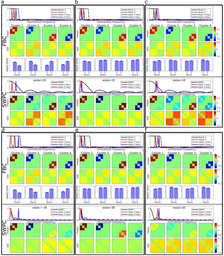
bioRxiv preprint first posted online Jul. 18, 2019; doi: http://dx.doi.org/10.1101/706838. The copyright holder for this preprint (which
 was not peer-reviewed) is the author/funder, who has granted bioRxiv a license to display the preprint in perpetuity.
 All rights reserved. No reuse allowed without permission.

 to the supplementary material). In addition, we have performed our analysis using different cluster
 numbers and provide this information in the supplementary material (Figures S2 through S10).

 Results
 As mentioned in the methods section, we designed several simulation scenarios using a multivariate
 Gaussian pdf to demonstrate the benefits of FBC compared to SWPC. In addition, we show the utilization
 of FBC on real data in a comparison of SZ with HC.

 Simulation Results

 All the simulation results are summarized in Figure 3. Each sub figure has 7 rows. The first and fifth rows
 demonstrate the normalized frequency response of covariance matrix for FBC (first row) and SWPC (fifth
 row). The second and third rows, demonstrate the mean and standard deviation (std) of simulations’ (each
 simulation was repeated 1000 times) centroids for FBC while the sixth and seventh rows demonstrate the
 same measures for SPWC results. Conceptually speaking, mean shows how the estimated values are close
 to the true values on average while std represent standard error of the estimators. The fourth row shows
 the total dwell time of each state in relation to the two filters. This information is exclusive to FBC and is
 absent in SWPC (SWPC is essentially one filter). Cluster 1 and 2 are the maximum and minimum values for
 state 1 (connectivity in state 1 oscillate between these values). Cluster 3 and 4 are the maximum and
 minimum values for state 2.

 In the first scenario (Figure 3 a through c), the SWPC window size (10 time points) covers the same
 frequency band as the two filters used in FBC. This scenario includes three specific situations. In the first
 situation, each state is located in one separate filter (Figure 3a) while in the second and third
 situations s are either in the first filter (Figure 3b) or in the second filter (figure 3c). Looking at the
 top three rows of Figure 3, we can make several observations. The means of estimated clusters are
 estimated very distinctly using FBC. i.e., cluster 1 and 2 only show state 1 while cluster 3 and 4 only
 shows state 2 . In contrast, if we look at SWPC results, mean of estimated clusters are only estimated
 distinctly when both states have low frequencies (Figure 3b). When the frequencies of the states are
 higher (Figure 3a and c) mean cluster are not distinct. For example, cluster means of Figure 3c for SWPC
 shows both state 1 and 2 in all clusters. Another interesting observation here is that for the case where
 the two states frequencies are located in separate filter bank frequency bands (Figure 3a), the dwell time
 figure for FBC clearly shows that cluster 1 and 2 happen more in first filter bank while the cluster 3 and 4
 happen more in the second filter. This shows that FBC can provide correct frequency specificity in the case
 where connectivity frequencies are distributed in different filter frequency bands. This point will be
 explored more in the discussion section.

 In the second scenario for the simulations, the window size is longer compared to the first scenario (30
 time point) and only covers the frequency band of the first filter (Figure 3 d through f). This scenario
 represents the case where SWPC window size is not chosen correctly (either because of technical
 limitations or user choice). i.e., the frequency pass band of the SWPC window does not cover all
 frequencies where state connectivity frequencies are located. This is clearly shown in Figure 3d and 3f
bioRxiv preprint first posted online Jul. 18, 2019; doi: http://dx.doi.org/10.1101/706838. The copyright holder for this preprint (which
 was not peer-reviewed) is the author/funder, who has granted bioRxiv a license to display the preprint in perpetuity.
 All rights reserved. No reuse allowed without permission.

 where at least one of the states has connectivity frequency outside the passband of the SWPC window.
 Looking at SWPC results in Figure 3d we can see that cluster 3 and 4 show very weak versions of state 2
 . In a more severe case where all states connectivity frequencies are outside the passband of SWPC
 (Figure 3f), all SWPC cluster mean values are very weak. Contrary to SWPC results, FBC mean values for
 cluster centroids are quite strong and similar to state 1 and 2 (Figure 2).

 A few other observations can be made regarding the std values. Based on the Figures 3 a through c we
 can see that SWPC has resulted in higher std values compared to FBC std values for null connectivity
 elements (matrix entries where connectivity is zero in each state). In contrast, looking at the second
 scenario results, we can see that using longer window sizes has resulted in lower std values when the
 actual connectivity frequency is very low. This is the case for Figure 3d first state and Figure 3e both states.
 But when the specific state has a higher frequency than the SWPC frequency band, the std values are
 noticeably higher for all matrices’ entries. This can be seen for the second state in Figure 3d and both state
 results in Figure 3f.
bioRxiv preprint first posted online Jul. 18, 2019; doi: http://dx.doi.org/10.1101/706838. The copyright holder for this preprint (which
 was not peer-reviewed) is the author/funder, who has granted bioRxiv a license to display the preprint in perpetuity.
 All rights reserved. No reuse allowed without permission.

 Figure 3. simulation results. Each figure (a through f) show the results from both FBC and SWPC analysis. The first four rows
 illustrate FBC related results while the last three rows illustrate SWPC results. The first and fifth row shows the connectivity
 frequency of each specific scenario in addition to the frequency response of filter banks (first row) and sliding window (the
 fifth row) used for the analysis. The second and sixth rows show the mean of estimated cluster centroids (i.e. connectivity
 states) from all simulations for FBC (second row) and SWPC (sixth row) approaches. The third and seventh rows show the
 std of the estimated cluster centroids for FBC (third row) and SWPC (seventh row) approaches. The fourth row shows the
 frequency profile of the estimated cluster centroids for FBC (this information is exclusive to the FBC approach and is one of
 this method strengths). Figures a through c is the scenario where the SWPC sliding window is chosen correctly (connectivity
 frequencies are included in the main lobe of the sliding window for all three cases). In these cases, SWPC has managed to
 estimate states correctly in the three cases but when at least one of the states has higher frequencies where SWPC main
 lobe has lower value (figure a and c), SWPC is not able to distinguish between different states well (the mean matrices show
 both state patterns). In contrast, FBC has managed to estimate the 2 states very distinctly (e.g. the state 2 pattern does not
 appear in both cluster 1 and 2 in figure c unlike SWPC results). In addition, FBC is showing superior std (i.e. lower) in these
 cases. Figures d through f illustrate the results from the second scenario where SWPC window size is not chosen correctly
 (either because of investigator mistake or Pearson correlation technical limitations). Apart from the case where both state
 connectivity frequency is in the passband of SWPC (figure e), SWPC is not able to estimate the two states well (i.e. low
bioRxiv preprint first posted online Jul. 18, 2019; doi: http://dx.doi.org/10.1101/706838. The copyright holder for this preprint (which
 was not peer-reviewed) is the author/funder, who has granted bioRxiv a license to display the preprint in perpetuity.
 All rights reserved. No reuse allowed without permission.

 values for means). In contrast, FBC does well in all three cases (high mean values). Apart from case e, where connectivity
 frequencies are very low and SWPC has an advantage over FBC, in the other 2 cases, std of FBC is superior too. One final
 note is that in the cases where the connectivity frequencies are in two separate bands (figures a and d) the connectivity
 frequency profiles resulted from FBC show that clusters 1 and 2 have lower frequency while clusters 3 and 4 have higher
 frequencies.

 Figure 4 shows the correlation between the estimated clusters and the true centroids (both positive and
 negative matrices shown in figure 2). Based on this figure we can see that in most cases FBC performs
 better (has a higher correlation) with the except of the case where the connectivity frequencies are well
 inside the SWPC frequency window (cases b and e). Thus, if even one of the states has a higher frequency
 than what is covered by the SWPC window, FBC perform better. In addition, compared to SWPC, FBC
 shows more robust performance (i.e. FBC performance is similar between different scenarios). Finally,
 FBC results seem to have less variation (spread of correlation values) compared with SWPC which has only
 low variation in cases b and d (essentially best case scenarios for SWPC).

 Figure 4 Correlation of estimated cluster centroids with ground truth for all simulations. The left figures show the results
 for the cases when the window size is 10 time points (cases a through c) while the right image is for the cases where the
 window size is 30 time points (cases d through f). As can be seen here FBC performs better for most of the cases, with the
 exception where the connectivity frequency is well in the band pass of SWPC sliding window (cases b and e; See Figure 3).
 In the cases where even one of the connectivity frequencies spread outside the SWPC window size (cases a, c, d and f) FBC
 performs better than SWPC. Note also that the FBC mean Correlation values remain mostly the same for all 6 cases. This
 observation combined with the fact that we are not able to know the correct window size, suggest FBC as a more robust
 solution.

 fBIRN results
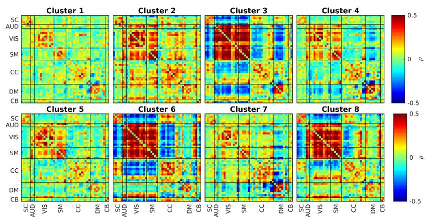
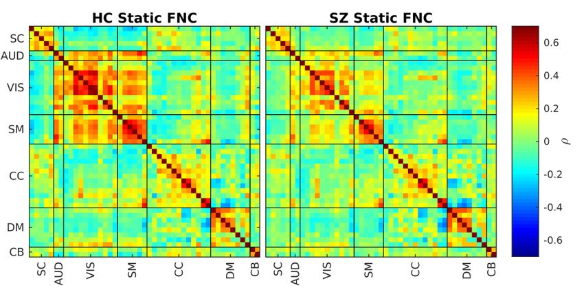
bioRxiv preprint first posted online Jul. 18, 2019; doi: http://dx.doi.org/10.1101/706838. The copyright holder for this preprint (which
 was not peer-reviewed) is the author/funder, who has granted bioRxiv a license to display the preprint in perpetuity.
 All rights reserved. No reuse allowed without permission.

 As mentioned in the method section, FBC is utilized to analyze the fBIRN data set. After calculating FBC
 values for all component pairs, these values are clustered into 8 clusters using the k-means method. The
 results can be seen in Figure 5. This figure first row shows the 8 cluster centroids. The second row shows
 the total dwell time for each cluster centroid for all filter banks. The third row shows the same total dwell
 time but overall filter banks with the aim of using these values to compare HC with SZ.

 Figure 5. fBIRN FBC results. The first row shows the cluster centroids of the 8 estimated clusters where the title shows the
 ratio of each state occurrence and range of each state centroid (e.g. for C1 -5.6e-01 is blue where 5.6e-01 is red). The second
 row shows each cluster frequency profile (dwell time of each cluster for each band) for HC and SZ separately. The third row
 compares the dwell time across all bands between HC and SZ (the title of each figure contains the comparison p-value where
 the significant ones are in bold font). The first observation we can make is that FBC has resulted in 3 states (states 2, 4 and
 8) which show opposite patterns to some other states (states 7,6 and 5 respectively). These opposite patterns are not visible
 within the SWPC results and all of them show a more high-pass frequency profile (possibly the reason these are not visible
 in the SWPC results). These opposite patterns might point to the presence of connectivity oscillation as designed in our
 simulations. Another observation we can make is that states 1 and 3 show very strong low-pass frequency profile where HC
 tend to spend more in state 1 while SZ spend more time in state 3. Interestingly, these two sates are very similar to the
 static connectivity calculated from HC and SZ separately (see Figure 6). Based on the total dwell time across all bands, we
 see that HCs tend to spend more time in state pairs 2 and 7 while SZ tend to stay more in states 5 and 8. States 8 is a finding
 exclusive to FBC and show negative connectivity between SM and SC/AUD/VIS domains. This state is quite similar to the
 state reported by (Yaesoubi et al., 2017) for SZ.
 Based on the total dwell time per filter bank figures (Figure 5 second row), we see that we essentially have
 3 types of clusters. The first clusters happen dominantly in the first filter bank (they have very low-pass
 nature). Cluster 1 and 3 belong to this category. The second category of clusters happen in middle
 frequencies (they have band-pass nature). Clusters 2, 4, 5, 6 and 7 belong to this category. Cluster 8 belong
 to the last category which happens dominantly in very high frequency (it has high pass-nature).

 Figure 6 shows the static FNC (FNC calculated over the whole time series using Pearson correlation) of HC
 and SZ groups separately. Looking at Figure 6, we can see that the HC group has a stronger positive
 connectivity block in AUD, VIS and SM functional domains compared to SZ static FNC. Comparing these
 results to the 2 low-pass clusters in Figure 5 (Cluster 1 and 3), we can see a resemblance between cluster
 1 and static FNC of HC (both have strong the strong connectivity block in AUD, VIS and SM domains) and
 cluster 3 and FNC of HC. This can also be verified using Figure 8. Based on this figure, HC static FNC highest
 correlation is with FBC cluster 1 while SZ static FNC has a higher correlation with FBC cluster 3. Another
bioRxiv preprint first posted online Jul. 18, 2019; doi: http://dx.doi.org/10.1101/706838. The copyright holder for this preprint (which
 was not peer-reviewed) is the author/funder, who has granted bioRxiv a license to display the preprint in perpetuity.
 All rights reserved. No reuse allowed without permission.

 observation that can enhance this comparison is that HC tends to spend significantly more time in Cluster
 1 compared to SZ (Figure 5 last row). SZ tend to stay more in cluster 4 compared to HC but this difference
 is not significant.

 Figure 6. sFNC for HC and SZ. Patterns are similar to these in both FBC (Figure 5) and SWPC (Figure 7) result. i.e. static
 connectivity information is present in dFNC results. In contrast to the SWPC method, FBC enable us to study the frequency
 profile of the estimated states and therefore we can identify states showing a static like nature (states 1 and 3 in the current
 work; Figure 5)
 Figure 7 shows the 8 clusters resulted from SWPC. Comparing Figure 7 with Figure 5, we can see that all
 the clusters resulting from SWPC are repeated in FBC results. This statement can be verified using Figure
 8. As seen in the aforementioned figure, all SWPC clusters have a high correlation with at least one of the
 FBC clusters. In contrast, 3 of FBC clusters are not visible in SWPC results, namely, clusters 2, 4 and 7. From
 These 3 clusters, clusters 2 and 4 have low dwell time in the first filter bank (where SWPC window in the
 frequency domain has the strongest value) and cluster 8 has very high dwell time in the last filter bank
 (where SWPC window has very low values in frequency domains). An additional observation we can make
 on these 3 clusters is that they are quite opposite of 3 other FBC clusters. Namely cluster 2 is opposite of
 cluster 1, cluster 4 is opposite of cluster 6, cluster 8 is opposite of cluster 5. This is quite similar to our
 simulation results (Figure 3).

 Looking at the comparison between HC and SZ dwell times of FBC results (Figure 5 last row), we can see
 that, from the 8 comparisons, 5 are significant after correcting for multiple comparisons. HCs tend to stay
 more in clusters 1, 2 and 7, while SZs tend to stay more in clusters 5 and 8. As mentioned previously,
 cluster 1, 2 and 7 are related while cluster 5 is related to cluster 8.
bioRxiv preprint first posted online Jul. 18, 2019; doi: http://dx.doi.org/10.1101/706838. The copyright holder for this preprint (which
 was not peer-reviewed) is the author/funder, who has granted bioRxiv a license to display the preprint in perpetuity.
 All rights reserved. No reuse allowed without permission.

 Figure 7. fBIRN SWPC results. As explained in the method section SWPC results are low-passed by nature. We can verify this
 claim by comparing these clusters with clusters resulted from FBC. SWPC clusters are highly similar to FBC clusters 1, 3, 5,
 6 and 7 (see Figure 8). Based on Figure 5, all these FBC clusters have a very low-pass frequency profile (dwell time at the
 first band is quite comparable to other bands). In contrast, FBC clusters 2, 4 and 8 have different frequency profiles. For FBC
 states 2 and 4 dwell time of the first band is low compared to other bands while for state 8, dwell time for the highest band
 is very high. Therefore, using SWPC, we are only able to investigate low-pass connectivity patterns where faster changes in
 connectivity (possibly can give us interesting information) can go undetected.
bioRxiv preprint first posted online Jul. 18, 2019; doi: http://dx.doi.org/10.1101/706838. The copyright holder for this preprint (which
 was not peer-reviewed) is the author/funder, who has granted bioRxiv a license to display the preprint in perpetuity.
 All rights reserved. No reuse allowed without permission.

 Figure 8. The similarity between sFNC and dFNC cluster centroids resulted from SWPC and those from FBC. The number in
 each matrix elements shows the order of FBC clusters similarity for each row (e.g. for SWPC C7 row, FBC C3 has the highest
 similarity with SWPC C7). We can see that sFNC calculated from HC is similar to FBC state 1 while SZ sFNC is similar to state
 3. Interestingly based on the FBC results (Figure 5), these two states show very low-pass frequency profile and HC tend to
 stay more in state 1 (p
bioRxiv preprint first posted online Jul. 18, 2019; doi: http://dx.doi.org/10.1101/706838. The copyright holder for this preprint (which
 was not peer-reviewed) is the author/funder, who has granted bioRxiv a license to display the preprint in perpetuity.
 All rights reserved. No reuse allowed without permission.

 connectivity domain is unclear at best and depends on the specific methods used. Many methods estimate
 connectivity (i.e. transform the activity domain into the connectivity domain) using highly nonlinear
 systems and therefore the frequency information is distorted in this transformation. For example, looking
 at the SWPC formula (Eq.1) we see that ( ) is subtracted from ( ) and the resulting value is divided by
 ( ). This part in itself distort the frequency profile of . In addition to calculating the correlation
 [ ( ) − ( )]⁄ ( ) is multiplied by [ ( ) − ( )]⁄ ( ) further distorting the frequency information.
 Therefore, using frequency information within the activity domain to infer frequency related information
 specific to connectivity is not straightforward. Some studies overlook this detail when studying
 connectivity frequency profile. For example, Li et. al. used frequency tiling in the activity domain to
 conclude that “oxygen correlation is band limited” (Li et al., 2015). In another study, Yaesoubi et al, used
 the wavelet transform to decompose the activity time series into different time-frequency bands and then
 calculate coherence. Several observations about connectivity frequencies are then made (Yaesoubi et al.,
 2017). In our view, these kinds of statements can be misleading as the frequency profile is not directly
 studied in the connectivity space and therefore it does not enable us to make claims about the
 connectivity frequency profile. Rather they show that connectivity is caused by signals (i.e. activity) from
 specific frequency bands.

 We believe to make claims about the connectivity frequency profile it is important to implement
 frequency tiling directly in the connectivity space and differentiate between the frequency profile of
 activity (estimated from time series themselves) and the frequency profile of the connectivity. The
 relationship between these two is not clear, so using knowledge about time series frequencies to make
 inferences regarding the connectivity frequency profile is not as straightforward as some studies suggest
 (Leonardi and Van De Ville, 2015).

 FBC performs frequency tiling in the connectivity domain

 In this work, we have proposed an approach called FBC to estimate dFNC which does not make any
 assumption about the frequency profile of connectivity. This is in contrast with SWPC, which applies a
 low-pass filter when calculating dFNC. Using k-means clustering to summarize FBC results, we found that
 in addition to states resulted from SWPC, we can estimate some other states exclusive to FBC (see Figure
 5). In addition, because of the frequency tiling nature of our method (which was implemented in
 connectivity domains) we are able to discuss the frequency profile of the estimated connectivity patterns.
 In many dFNC studies, it is reported that one state (typically from SWPC) tends to be quite similar to the
 static connectivity (Damaraju et al., 2014; Faghiri et al., 2018). In this study, we see that 2 states have
 strong low frequency profiles (states 1 and 3; see Figure 5). State 1 is quite similar to sFNC resulted from
 HC individuals while the other state, state 3, is similar to sFNC resulted from SZ (see Figure 8 for correlation
 between different states). One possible conclusion from this observation is that FBC enables us to
 distinguish between states that show more static like behavior (states that show low-pass frequency
 profile) and others which are more dynamic (states that show high or band-pass frequency profile). This
 feature of FBC can be utilized so that we have a full picture of FNC in all its frequencies. i.e, study both
 static and dynamic FNC patterns simultaneously. One possible modification of our approach is using very
 narrow passband for the first filter bank (which includes pure sFNC) so that the first filter represents lower
 frequencies of FNC (more static like FNC).
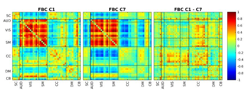
bioRxiv preprint first posted online Jul. 18, 2019; doi: http://dx.doi.org/10.1101/706838. The copyright holder for this preprint (which
 was not peer-reviewed) is the author/funder, who has granted bioRxiv a license to display the preprint in perpetuity.
 All rights reserved. No reuse allowed without permission.

 sFNC repeats in higher frequencies with lower Cognitive Control connectivity

 Similar to the states reported in our earlier work (Damaraju et al., 2014), several of the states resulted
 from SWPC approach (Figure 7) are quite similar to each other (states that show similar patterns to overall
 sFNC). We can see two states similar to these in FBC results too (namely states 1 and 7). Unlike SWPC
 results, here we can see that while state 1 shows a very strong low-pass frequency profile, state 7 shows
 a more uniform frequency distribution across bands (Second row Figure 5). Again because of the
 frequency tiling of FBC, we have some added information in regard to the frequency profile of connectivity
 patterns that we can investigate. Figure 9 illustrates these two states while showing the difference
 between their normalized versions. As seen in the rightmost of Figure 9, cluster 7 has lower CC
 connectivity in general. One possible observation we can make here is that cluster 1 (which is quite similar
 to HC sFNC and has a very low-frequency profile) occurs in higher frequencies in the form of cluster 7 with
 smaller CC connectivity values. We speculate that CC (especially intraconnectivity within CC components)
 are lower in higher frequencies. This point needs further examination in future works.

 Figure 9. A close look at FBC clusters 1 and 7. The rightmost figure shows the difference between cluster 1 (left) and cluster
 7 (middle). The positive sign in each entry for the difference matrix indicate the entries where C1 is positive. Based on this
 figure we can see that C1 is very similar to C7 but it has higher connectivity values for CC (both connectivity within CC and
 between CC and other networks). This can mean that sFNC connecitivity patterns are repeated in higher frequencies too
 but with lower connectivity in CC.

 Anticorrelation between somatomotor and subcortical/visual/auditory networks

 FBC has resulted in two unique states, 5 and 8, which are not visible in SWPC clusters (no SWPC cluster
 show the highest correlation with these states). SZ tend to significantly spend more times in these two
 states compared to HC (P
bioRxiv preprint first posted online Jul. 18, 2019; doi: http://dx.doi.org/10.1101/706838. The copyright holder for this preprint (which
 was not peer-reviewed) is the author/funder, who has granted bioRxiv a license to display the preprint in perpetuity.
 All rights reserved. No reuse allowed without permission.

 controls (D'Ausilio et al., 2009; Londei et al., 2010). A reduction in connectivity between these regions in
 SZ has been reported in the past years (Berman et al., 2016; Kaufmann et al., 2015). In our work, we do
 not find a reduction in the connectivity between SM and VIS/AUD network, rather we show that SZ spends
 more time in states showing strong anticorrelation between these networks.

 Dynamic connectivity highlights oscillations between two opposite patterns

 Another observation we can make based on the states estimated using FBC (Figure 5) is that there are
 pairs of states (undetected by SWPC) which show opposite connectivity patterns (SWPC identifies only
 one of these). In our case, states 2, 4 and 8 show opposite connectivity patterns of states 7, 6 and 5
 respectively. One interesting insight about states 2, 4 and 8 is that they exhibit a more high-pass frequency
 profile compared to the other states. This is possibly the reason that these states are not estimated using
 SWPC. It is unlikely that these opposite patterns are due to an alteration in phase caused by the analysis
 since, as mentioned in the methods section, we used forward-backward filtering. Another explanation can
 be that these states are spurious estimations caused by the high-frequency nature of the filter banks as
 discussed by (Leonardi and Van De Ville, 2015). We cannot rule out this possibility completely but because
 these states show the opposite patterns of some other low-pass states this is unlikely. To further
 investigate, we removed the low frequency information of SWPC with different high-pass filters (forward-
 backward filtering) and then performed k-means clustering. Figure 10 shows the resulting clusters using
 different high pass filters. When removing the low frequency information, we obtain these opposite
 clusters (e.g. C3, Figure 10, quite similar to FBC cluster 2). Another possible explanation for these opposite
 patterns is that, similar to how the simulation was designed, the dynamic connectivity patterns oscillate
 between two opposite patterns. Unlike the simulation, the negative patterns (states 2, 4 and 8) show a
 higher frequency profile compared to their more low-pass counterparts, but this could reflect asymmetric
 oscillatory behavior (e.g. more rapid return from the negative patterns). This is an interesting observation;
 however future work should be designed to further explore the possibility that connectivity indeed
 oscillates between two opposite connectivity patterns. In addition, the biological/clinical meaning of this
 view should be explored further.
bioRxiv preprint first posted online Jul. 18, 2019; doi: http://dx.doi.org/10.1101/706838. The copyright holder for this preprint (which
 was not peer-reviewed) is the author/funder, who has granted bioRxiv a license to display the preprint in perpetuity.
 All rights reserved. No reuse allowed without permission.

 Figure 10. high-passed SWPC results. To verify FBC results we removed low frequency information of SWPC using different
 high-pass filters and then used k-means clustering. The first row is essentially unfiltered SWPC results while the next three
 rows are SWPC results using different filters. As seen in the last three row we have clusters similar to FBC clusters in SWPC
 results too (cluster 3, 4 and 8). The only reason these clusters were not estimated using unfiltered SWPC is because SWPC
 frequency response function attenuate all frequencies above zero even in its band-pass.

 A systematic view of estimations

 We believe that any analysis steps (including statistical estimators) can be viewed as a system and benefit
 from the extensive work done in system design field (Bentley et al., 2000). In this work, we examined
 SWPC and proposed an approximate system diagram for it (Figure 1.a). This way of thinking about SWPC
 facilitated our conclusion that SWPC has a low-pass filter inherent to its formula and led to our proposed
 more comprehensive FBC solution involving the use of a filter bank instead of a low-pass filter (Figure 1).
 The use of filter banks as proposed in the current work is only one possibility, for future work we can use
 custom h(t) modules to extract specific information. For example, one possible choice is wavelet
 transform in the place of subsystem 2 (wavelet can be viewed as a system itself). Another possibility is to
 improve SWPC by replacing its h(t) with an IIR low-pass filter with very sharp transition and flat band-pass
 (in contrast with SWPC with rectangular window where the frequency response of the filter is sinc like).
 This is in line with previous works where it has been suggested that SWPC window shape can be
 modulated to achieve better results (Mokhtari et al., 2019).

 Limitations

 The first limitation of the FBC approach is the subsystem used to transform activity space to connectivity
 space (Figure 1). In this system, we have used a window to calculate the mean and standard deviation.
 the problem arises when mean and std move faster than what the window can track. In this case, our
 estimations will be sub-optimal. To remedy this, we can use more instantaneous methods suggested for
 estimating correlation in future work (Shine et al., 2015). Another limitation of this method is the
 possibility of noise contamination in the higher frequencies. This is certainly a valid issue, though our goal
 in this work was to refrain from making any strong assumption about connectivity frequencies. The reason
bioRxiv preprint first posted online Jul. 18, 2019; doi: http://dx.doi.org/10.1101/706838. The copyright holder for this preprint (which
 was not peer-reviewed) is the author/funder, who has granted bioRxiv a license to display the preprint in perpetuity.
 All rights reserved. No reuse allowed without permission.

 behind this decision was that we have no solid prior knowledge about connectivity frequency. In fact, to
 the best of our knowledge, this work is the first one that differentiates between activity and connectivity
 frequency profiles. Future investigators can utilize our proposed approach to study specific frequency
 bands.

 Conclusion

 In this work, we proposed a new approach to estimate dFNC called FBC. Our proposed approach does not
 make any strong assumption about connectivity frequency (unlike SWPC) and performs the frequency
 tiling in the connectivity domain (in contrast to previous works were frequency tiling was implemented in
 the activity domain). FBC aims to estimate connectivity in all frequencies and it enables us to investigate
 connectivity patterns frequency profiles. Using simulations, we showed that FBC is able to estimate even
 high-frequency connectivities in addition to providing information about the estimated connectivity
 frequencies. Utilizing FBC, we analyzed an fMRI dataset including HC and SZ. We found both sFNC and
 SWPC dFNC states using FBC in addition to some new connectivity states undetected by SWPC (possibly
 because of their high-pass nature). Finally, FBC points to a possible (new) view for connectivity. In this
 view, data oscillate between two opposite connectivity patterns. This view should be further explored in
 future work.

 Conflicts of interest
 Authors declare no conflict of interests.

 Acknowledgements
 Data collection was supported by the National Center for Research Resources at the National Institutes of
 Health (grant numbers: NIH 1 U24 RR021992, NIH 1 U24 RR025736-01, R01EB020407, P20GM103472,
 P30GM122734) and the National Science Foundation (1539067);
bioRxiv preprint first posted online Jul. 18, 2019; doi: http://dx.doi.org/10.1101/706838. The copyright holder for this preprint (which
 was not peer-reviewed) is the author/funder, who has granted bioRxiv a license to display the preprint in perpetuity.
 All rights reserved. No reuse allowed without permission.

 References:
 Allen, E.A., Damaraju, E., Plis, S.M., Erhardt, E.B., Eichele, T., Calhoun, V.D., 2014. Tracking whole-brain
 connectivity dynamics in the resting state. Cereb Cortex 24, 663-676.
 Bentley, L.D., Dittman, K.C., Whitten, J.L., 2000. Systems analysis and design methods. Irwin/McGraw
 Hill.
 Berman, R.A., Gotts, S.J., McAdams, H.M., Greenstein, D., Lalonde, F., Clasen, L., Watsky, R.E., Shora, L.,
 Ordonez, A.E., Raznahan, A., Martin, A., Gogtay, N., Rapoport, J., 2016. Disrupted sensorimotor and
 social-cognitive networks underlie symptoms in childhood-onset schizophrenia. Brain 139, 276-291.
 Boashash, B., 2015. Time-frequency signal analysis and processing: a comprehensive reference.
 Academic Press.
 Calhoun, V.D., Adali, T., Pearlson, G.D., Pekar, J.J., 2001. Spatial and temporal independent component
 analysis of functional MRI data containing a pair of task-related waveforms. Hum Brain Mapp 13, 43-53.
 Camchong, J., MacDonald, A.W., 3rd, Bell, C., Mueller, B.A., Lim, K.O., 2011. Altered functional and
 anatomical connectivity in schizophrenia. Schizophr Bull 37, 640-650.
 Chang, C., Glover, G.H., 2010. Time-frequency dynamics of resting-state brain connectivity measured
 with fMRI. NeuroImage 50, 81-98.
 D'Ausilio, A., Pulvermuller, F., Salmas, P., Bufalari, I., Begliomini, C., Fadiga, L., 2009. The motor
 somatotopy of speech perception. Curr Biol 19, 381-385.
 Damaraju, E., Allen, E.A., Belger, A., Ford, J.M., McEwen, S., Mathalon, D.H., Mueller, B.A., Pearlson,
 G.D., Potkin, S.G., Preda, A., Turner, J.A., Vaidya, J.G., van Erp, T.G., Calhoun, V.D., 2014. Dynamic
 functional connectivity analysis reveals transient states of dysconnectivity in schizophrenia. Neuroimage
 Clin 5, 298-308.
 Di Martino, A., Scheres, A., Margulies, D.S., Kelly, A.M., Uddin, L.Q., Shehzad, Z., Biswal, B., Walters, J.R.,
 Castellanos, F.X., Milham, M.P., 2008. Functional connectivity of human striatum: a resting state FMRI
 study. Cereb Cortex 18, 2735-2747.
 Erdeniz, B., Serin, E., Ibadi, Y., Tas, C., 2017. Decreased functional connectivity in schizophrenia: The
 relationship between social functioning, social cognition and graph theoretical network measures.
 Psychiatry Res Neuroimaging 270, 22-31.
 Erhardt, E., Allen, E., Damaraju, E., Calhoun, V., 2011. On network derivation, classification, and
 visualization: a response to Habeck and Moeller. Brain Connect.
 Faghiri, A., Stephen, J.M., Wang, Y.P., Wilson, T.W., Calhoun, V.D., 2018. Changing brain connectivity
 dynamics: From early childhood to adulthood. Hum Brain Mapp 39, 1108-1117.
 Hutchison, R.M., Womelsdorf, T., Allen, E.A., Bandettini, P.A., Calhoun, V.D., Corbetta, M., Della Penna,
 S., Duyn, J.H., Glover, G.H., Gonzalez-Castillo, J., Handwerker, D.A., Keilholz, S., Kiviniemi, V., Leopold,
 D.A., de Pasquale, F., Sporns, O., Walter, M., Chang, C., 2013a. Dynamic functional connectivity:
 promise, issues, and interpretations. Neuroimage 80, 360-378.
 Hutchison, R.M., Womelsdorf, T., Gati, J.S., Everling, S., Menon, R.S., 2013b. Resting-state networks
 show dynamic functional connectivity in awake humans and anesthetized macaques. Hum Brain Mapp
 34, 2154-2177.
 Iraji, A., Deramus, T.P., Lewis, N., Yaesoubi, M., Stephen, J.M., Erhardt, E., Belger, A., Ford, J.M.,
 McEwen, S., Mathalon, D.H., Mueller, B.A., Pearlson, G.D., Potkin, S.G., Preda, A., Turner, J.A., Vaidya,
 J.G., van Erp, T.G.M., Calhoun, V.D., 2019a. The spatial chronnectome reveals a dynamic interplay
 between functional segregation and integration. Hum Brain Mapp 40, 3058-3077.
 Iraji, A., Fu, Z., Damaraju, E., DeRamus, T.P., Lewis, N., Bustillo, J.R., Lenroot, R.K., Belger, A., Ford, J.M.,
 McEwen, S., Mathalon, D.H., Mueller, B.A., Pearlson, G.D., Potkin, S.G., Preda, A., Turner, J.A., Vaidya,
You can also read