Preliminary Impacts of Wind Power Integration in the Hydro-Quebec System
←
→
Page content transcription
If your browser does not render page correctly, please read the page content below
W IND E NGINEERING VOLUME 36, N O . 1, 2012   PP   35-52                                            35

Preliminary Impacts of Wind Power Integration in
the Hydro-Quebec System
André Robitaille1, Innocent Kamwa2, Annissa Heniche Oussedik2, Martin de Montigny2,
Nickie Menemenlis2, Maurice Huneault2, Alain Forcione2, Richard Mailhot3, Jacques
Bourret4 and Luc Bernier4
1Hydro-Québec    Production, 75 boul René Lévesque Ouest 9e étage, Montréal, Québec, Canada,
H2Z 1A4 E-mail: robitaille.andre@hydro.qc.ca
2Institut de recherche d’Hydro-Québec (IREQ), 1800 boul. Lionel-Boulet, Varennes, Québec, Canada,

J3X 1S1
3Hydro-Québec TransÉnergie, C.P. 10000, Succ. Pl. Desjardins, tour Est, étage B1,

Centre Hydro, Complexe Desjadins, Montréal, Québec, Canada, H5B 1H7
4Hydro-Québec Distribution, 75 boul René Lévesque Ouest, 22e étage, Montréal, Québec, Canada,

H2Z 1A4

   ABSTRACT
   Recent studies undertaken by Hydro-Québec evaluate three aspects of the integration of
   wind generation on their system reliability/security. In an operations setting, the impacts on
   intra-hourly operating reserves and on extra-hourly balancing reserves are examined. On
   an operations planning horizon, the wind power capacity credit is evaluated for winter peak
   loading conditions, when very cold temperatures risk disabling part of the wind generation.
   Depending on the study, various mathematical tools were used to generate the statistical
   characteristics of the load and anticipated wind generation: time-series analysis, wind
   simulation at new/future wind plant sites, power system simulation and a posteriori
   determination of forecast errors. However, in each case the measure used to quantify the
   impact of wind generation has been related to the change in the variance of the total system
   uncertainty as a result of the addition of wind power generation.

   Keywords: Wind-hydro, impacts, reliability, reserves, load-following, regulation, balancing,
   capacity credit

1. INTRODUCTION
Hydro-Québec (HQ) has taken advantage of the vast hydropower potential on its territory to
develop a green and renewable energy base. Its installed hydro capacity stands at 97% of its
total generation capacity of about 40 GW. It is now turning increasingly to wind power as a
complementary source of renewable energy. Accordingly, it has been decided that the
installed wind capacity will reach 10% of that of hydro by 2016, or about 4000 MW, and that this
ratio will most likely be maintained thereafter.
   Presently, the impacts of this rapid integration of wind power on the power system are
being evaluated. System reliability/security issues have been prioritized, while technical and
economical effects on water management and market-related issues are targeted for a
second phase of the study. Accordingly, the reliability/security-related aspects considered
and presented here are the impacts of wind power on
36                    P RELIMINARY I MPACTS   OF   W IND P OWER I NTEGRATION   IN THE   H YDRO -Q UEBEC S YSTEM

1.   Operating reserves, to mitigate the effects of sudden changes in the power system
     (contingencies) and of slower frequency deviations due to load and wind generation
     variability in the intra-hourly time frame. These reserves essentially address power
     system security.
2. Balancing reserves, to mitigate the consequences of inherent load and wind generation
     forecast errors over the time horizon of 1 to 48 hours. These reserves essentially address
     economic aspects of short-term supply adequacy.
3. System capacity adequacy, to address reliability aspects of long term supply adequacy
     taking into account coincident load and wind power series with real weather conditions,
     and further the forced outages of the wind turbines induced by very cold temperatures
     (under −30°C).

     Important variables influencing the amount of required reserves are the capacities and
geographical dispersion of the wind power plants, the magnitude and profile of the load, the
coincidence between load and wind power, and the (winter) meteorological conditions at
peak load. These impacts and underlying variables are not specific to a massively hydro-
electric system; nevertheless, a thorough analysis of each of these aspects sheds light on the
advantages that a large hydro capacity can offer in efficiently integrating wind power in the
electrical system.
     This paper summarizes three studies undertaken at HQ [1−5], each assessing one of the
above impacts. The studies are based on the addition into the power system of 3000 MW of
wind power capacity over 23 wind power plants, either presently built or under contract to be
built by 2016. Figure 1 illustrates their locations in the province.

               Figure 1: Locations of the 23 wind power plants considered in the study.
W IND E NGINEERING VOLUME 36, N O . 1, 2012   PP   35-52                                      37

2.PRELIMINARIES
2.1. Reserve types and their magnitudes at HQ
HQ maintains six types of reserves, which are grouped in two broad categories as shown in
Table 1.
   These are listed below from the most to the least fast-acting.
   The first five types taken together constitute the operating reserves. Of these, the first
three react to contingencies. Stability or spinning reserves, typically 1000 MW, serve to
stabilize power/voltage immediately following a system contingency. They are sized to cover
60% of the largest single loss of generation. The 10-minute and 30-minute reserves further aid
in the recovery of system frequency in the minutes following the contingency. The 10-minute
reserves, which consist of non-firm sales, interruptible load and a large portion of stability
reserves, typically are also set around 1000 MW. The 30-minute reserves, typically about
500 MW, cover 50% of the second most severe single loss of generation.
   The next two types of reserves act to counter the variability of system load and wind
generation. Frequency regulation reserves use the automatic generation control (AGC) to
counter slow frequency variations in a time frame of minutes; they operate over a 500 MW
(minimum) modulation range. Load-following reserves operate over a longer time frame
within the hour. They do not have a strictly defined standard, since this function can be
performed practically without any constraint on the amount of power that can be obtained.
This is because most often power is readily available in capacity and ramping rate from HQ’s
large hydro-generation base.
   The energy-balancing reserves, or simply balancing reserves, act to counter uncertainties
in load and wind generation forecasts over a time horizon of 1 to 48 hours ahead. They can
vary from 1500/1200 MW (winter/summer) in the day-ahead time frame to 500 MW in
real-time two-hours ahead. These reserves consist mostly of calls to non-firm export sales,
interruptible load, gas turbines, etc. Since HQ participates actively in neighboring electricity
markets through asynchronous links, balancing reserves aim at assuring both the short-term
supply adequacy for its customers and the honoring of commercial commitments in those
markets.

2.2. Wind power modeling
To support the realization of its integration studies, HQ simulated the important variables at
each wind power plant site under consideration. Hourly time series of wind speed, air
temperature and wind generation covering a period of 36 years (1971−2006) were
reconstituted based on historical measurements from Environment Canada weather
stations and meteorological mats, wind power plant layouts, local topography information,
and diagnostic extrapolation models. These series were validated in two ways. First, as
3 wind plants were already in operation in 2009, HQ extended the time series for 3 years and
compared them with actual measurements at those sites [6] [7]. Secondly, due to the

                                       Table 1: Reserve types

                            Operating reserves                      Balancing reserves
 For contingencies        For load and wind power          For load and wind power forecast
                            variability                      uncertainties (horizon 1–48 hours)
 Stability reserve        AGC (regulating, minutes)        Balancing Reserves
   10 minutes               Load following
   30 minutes               (intra-hour)
38 P RELIMINARY I MPACTS OF W IND P OWER I NTEGRATION IN THE H YDRO -Q UEBEC S YSTEM
importance of the quality of the time series when the wind turbines could be shutdown under
−30°C, Hydro-Quebec proceeded to cross-validate and update the reconstituted data for
14 historical peak load events using a high resolution numerical weather forecast model [8].
3. FREQUENCY REGULATION AND LOAD-FOLLOWING RESERVES
3.1. Introduction to the HQ approach
Within the one-hour time frame, a preliminary analysis rapidly identified that the
contingency-related reserve categories are not sensitive to wind energy integration. That
is essentially because the wind plants are limited in size (less than 200 MW) and are
geographically dispersed over 1000 km. The loss of a wind power plant, or more likely of
only part of a plant, would have little impact on the stability of the system. Hence in this
time frame, only the AGC and load-following reserve capacities deserve further
investigation.
Two methodologies for computing additional regulation capacity requirements due to the
presence of wind power were applied to the Quebec network: that developed by the Oak
Ridge National Laboratory (ORNL) [9] and that proposed by the Bonneville Power
Administration (BPA) for its Rate Case 2010 [10]. These require regulation signals as input. For
the generation of regulation signals, REGAGC and REGLF, two distinct approaches were
considered, one based on statistical time-series analysis and the other on simulation. These
elements are illustrated in Figure 2 below, with the signal-generating functions in the top
boxes, the capacity adjustment function in the central box, and a look at results highlighting
the impacts of wind generation in the lower box. Each of these elements is presented in the
following sections.
After reviewing the pros and cons of each, HQ’s ISO, TransÉnergie (TÉ), opted for the
simulation approach for the following reasons:
Load data
Load
time-series
Computation of Computation of
regulation signals using regulation signals Wind data
analytical methods using the simulator
Wind
time-series
REGAGC REGAGC Network data
REGLF REGLF
Computation of
additional regulation
reserves
BPA and ORNL
Impacts
Figure 2: Computational scheme for the impact of wind power generation on the AGC and LF reserve
capacity requirements.W IND E NGINEERING VOLUME 36, N O . 1, 2012 PP 35-52 39
1. Unlike in most other North-American jurisdictions, TÉ’s Area Control Error (ACE) is
dependent only on the frequency deviation and not on tie-line power imbalances. The
analytical approach does not use and thus cannot handle frequency deviation whereas
the simulation approach can.
2. Simulation provides a means to monitor many other impacts of wind power such as the
frequency of stop-starts, the efficiency degradation of AGC units and, in particular, the
AGC’s regulating range. The simulation approach is currently under development at IREQ
in a simulator called SIRE [2], further described in Section 3.2.2. It reproduces the power
system behavior in the presence of wind generation over a long time horizon with a
1-minute resolution.
With the two methodologies fed successively with input signals from the two regulation
signal generating approaches, four series of results are generated. These results are presented
and compared in a final section.
3.2. Preparation of simulation data
In preparation of the computation of reserve requirements, regulation signals were generated
based on the following two approaches.
3.2.1. Signals based on load and wind time series
Contrary to a simulation approach, this approach is not based on using a detailed modeling of
the underlying power systems. In fact, it consists in applying analytical methods to
chronological series of the demand and wind generation over a number of years [19, 20]. For
our study, hourly demand and wind generation forecasts were derived for the year 2016 as
follows. The Load Serving Entity first derived its 2016 demand forecasts based on the actual
2006 demand profile and on realistic load growth assumptions. Then, 11 years of hourly
demand data were simulated from this baseline forecast to best fit the climatologic conditions
observed from 1995 to 2006. Assuming similar meteorological conditions in 2016, the simulated
2016 hourly demand should mimic quite accurately the time-series generated in the long term
statistical analysis.
Similarly, the hourly wind generation data comes from 11-year historical reconstitutions of
the anticipated 3000-MW wind plants generation capacity [6, 7] as described in Section 2.2.
Following studies by BPA and the California Independent System Operator, real-time hour-
ahead wind forecasts are based on a simple 2 hour persistence model. However, for the
simulator-based studies, a 1 hour persistence model was deemed more realistic in the Hydro-
Québec Energy Management System (EMS) context.
The minute by minute demand and wind generation data were then interpolated
according to [1]. Table 2 summarizes some of the typical features of the minute by minute data
of the long term demand and wind generation time series. Generally speaking, wind
generation proportionally has more variability and less real-time predictability than the
load.
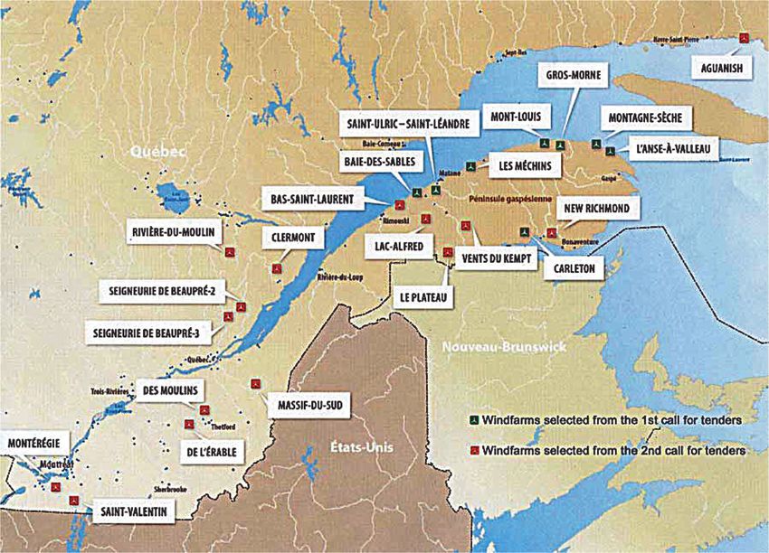
Figure 3 illustrates the overall characteristics of wind generation integrated into the HQ
network. The daily maximum (blue) and minimum (red) values of the hourly penetration
rates are shown in Figure 3 (a) (i.e. 365 values per year for each curve). Figure 3 (b) presents
the daily maximum (blue) and minimum (red) hourly ramping of the wind generation. The
overall peak load of 41,126 MW occurred on January 2004, while the absolute minimum load
of 13 998 MW was reached in June 1996. The highest penetration rate is about 18% at the
hours when the high wind generation is coincident with the low load.40 P RELIMINARY I MPACTS OF W IND P OWER I NTEGRATION IN THE H YDRO -Q UEBEC S YSTEM
Table 2: Summary statistics of minute by minute data
from November 1, 1995 to October 31, 2006
In % with respect In % with respect
Demand1 to the Mean to the max
(MW) Demand Demand
Standard deviation of variability 1 min 38.5 0.2 0.1
Standard deviation of variability 1 h 837 4 2
Absolute average real-time 522 2.5 1.2
forecasting error (1 h look-ahead time)
Standard deviation of real-time 686 3.2 1.6
forecasting errors (1 h look-ahead time)
Wind In % with respect In % with respect
generation1 to mean wind to rated wind
(MW) generation generation
Standard deviation - variability 1 min 7.5 0.7 0.3
Standard deviation - variability 1 h 171 15.6 5.7
Absolute average real-time 202 18.4 6.7
forecasting error (2 h-persistence model)
Standard deviation of real-time 227 21 7.6
forecasting errors (2 h-persistence model)
Mean Demand = 21 204 MW,
1
Max Demand = 41 774 MW;
Mean Wind = 1 099 MW, Max Wind = 2 801 MW, Rated Wind = 3000 MW.
3.2.2. Signals generated by the Hydro-Québec power grid simulator
Other power grid simulators have been developed for specific needs seemingly similar to ours.
A simulator developed by KEMA [11] is used mainly for market and storage systems modeling.
The e-terraSimulator model proposed by AREVA [12] can simulate real-time power grid
control, but it is designed for operator training. These simulation tools are ill-suited for fast
simulation of long time periods multi-scenarios.
The new simulator developed by Hydro-Québec, called SIRE, is devoted to the
quantification of the impacts of wind integration on quantities related to power grid control in
the context of the transmission service provider. It is based on a multi-agents framework, built
using a specification published by Sandia National Laboratories [13]. It was designed for fast
simulation of the planning and real-time phases, while taking into account security and
regulation rules of the transmission system provider.
This study has been made possible by the availability of comprehensive and accurate data
from three sources:
– One year duration (year 2006) of actual and forecasted global demand
(i.e. domestic load plus power exchanges with neighboring grids) obtained from the
EMS/SCADA historian.
– For each wind power plant under consideration, one year duration (year 2006) of
simulated time series of wind power generation [6, 7].
– One year of hourly topologies of the network, in the form of load flow cases, taken
from the state estimator historian.
These input feed the simulator to produce a complete simulation of the operation of the
power system. Conventional generation is allocated based on the historical commitment
ranks of the units in response to load and wind generation. Given generation and load patternsW IND E NGINEERING VOLUME 36, N O . 1, 2012 PP 35-52 41
(a) Hourly penetration rate
18
16
14
12
10
%
8
6
4
2
0
1996 1997 1998 1999 2000 2001 2002 2003 2004 2005 2006 2007
(b) Hourly wind generation ramping (wind base = 3000 MW)
30
20
10
Hour %
0
−10
−20
−30
1996 1997 1998 1999 2000 2001 2002 2003 2004 2005 2006 2007
Figure 3: (a) Daily maximum and minimum of hourly penetration; (b) Ramping rates in % of rated
wind generation.
and a description of the network, all the electrical variables in the network are computed
using an AC power flow.
This signal-generating approach has the advantage of modeling all the network variables
and the constraints imposed by regulation rules and operational limitations such as the
regulating range and up-down margins of the AGC system. In the analytical time series signal-
generating approach, these impositions would have gone unconsidered.
3.3. Reserve capacity evaluation
Independently of the approach used for generating regulation signals time series data, to date
measures to quantify the impact of wind power generation on reserve capacity requirements
have been based on statistical methods (most notably in [16]). Most often, the adopted
measure has been the difference between the variance of the variability of the net load,
defined as the load minus wind generation, versus that of the load alone. Their application and42 P RELIMINARY I MPACTS OF W IND P OWER I NTEGRATION IN THE H YDRO -Q UEBEC S YSTEM
detailed assessment on the HQ network, in the context of wind integration impact studies for
the intra-hourly time horizon, was reported in [1].
The two methodologies considered here, introduced earlier, are described below. We note
important differences between them: from a general viewpoint they pursue different
philosophies; in particular one assumes statistical independence of the input signals whereas
the other considers the covariance between the input signals.
3.3.1. The ORNL method based on standard deviation
This methodology, developed by ORNL [9], was applied to Nordic countries in [16] to assess the
impacts of wind integration on reserves. The main idea is to use the increase in the standard
deviation of the regulation signals as a measure of the impact of wind integration. More
precisely, if one assumes that the variability of load and wind are normally distributed and
uncorrelated, then the corresponding regulation signals will also be normally distributed and
uncorrelated. Then
σ 2 (REG NL ) = σ 2 (REG L ) + σ 2 (REGW ) (1)
where σ(REGNL) is the standard deviation of signal REG. REG can represent the regulation
signal associated with Automatic Generation Control (AGC) or load-following (LF), and X
represents load or wind. The NL, L and W indices refer to net-load, load and wind respectively.
The additional regulation requirement to cover the accrued net load variability brought by
the integration of wind generation, ∆REG ORNL (Wind), is then determined as
∆REG ORNL (Wind ) = n × ( (σ 2 (REG L ) + σ 2 (REGW ) − σ (REG L ) ) (2)
Here n is a suitable number selected to cover the risk associated with almost all occurrences
of wind variability. Since the faster acting reserves cannot rely on backup actions, their values
of n must be higher than those of slower reserves. Hence, typically n is chosen between 4 and
6 for AGC and between 2 and 2.5 for load-following. More specifically, in order to cover most of
the variability, Hydro-Quebec adopted n = 4 for AGC and n = 2 for load-following.
3.3.2. The BPA method based on an allocation formulation
This approach [10] was first proposed by BPA for wind generation projects in their control area
[14]. The principle is to establish the total reserve capacity requirement, and then to attribute
to the proportions that the wind and load components each contributes to the total using the
99.5%
covariance allocation concept [2] [15]. The total regulation capacity requirement REG NL ,
whether for AGC or for load-following, was computed to cover the net load variability at a
99.5% exceedance level, based on the regulation signal statistical characteristics over the
corresponding time frames, i.e.
Prob REG NL
99.5%
≥ REG NL = 0.995 (3)
where REG NL, is the net load regulation defined as a random variable. The value 0.995 of the
exceedance level would correspond to an n of 2.58 should the variability be Gaussian. The
relative contribution of each component is given by:W IND E NGINEERING VOLUME 36, N O . 1, 2012 PP 35-52 43
cov(−REGW , REG NL ) σ 2 (REGW ) + cov(−REGW , REG L )
WindShare = =
σ 2 (REG NL ) σ 2 (REG NL )
(4)
cov(REG L , REG NL ) σ 2 (REG L ) + cov(REG L , −REGW )
LoadShare = =
σ 2 (REG NL ) σ 2 (REG NL )
where
COV(X,Y) represents the covariance between the variables X and Y,
COV (–X,Y) = COV(Y, –X), confirms the equality of the covariances with commuted
arguments,
REGNL = REGL _ REGW expresses the regulation on the net load as the difference between
those on the load and the wind components.
The covariance coefficients in equation (4) account for the correlation between wind and
load regulation signals. Contrary to the ORNL method, equation (4) was applied in this study
to data collected at each hour (h) of the day, resulting in diurnal cycles of wind and load shares
of AGC and load-following. Given the hourly relative wind and load shares, the absolute
contribution of each entity (in MW) was obtained as follows:
WindShareMW (h) = WindShare (h ) × REG NL
99.5%
(h)
(5)
LoadShareMW (h ) = LoadShare (h ) × REG NL
99.5%
(h)
For year 2006, Figure 4 shows diurnal cycles of wind and load shares of the forecasted
load-following obtained from the SIRE simulator. Note that at this stage the wind and load
shares are expressed in per unit, such that their sum is exactly equal to one.
Figure 5 illustrates the diurnal contribution of each entity in MW. In this case the forecasted
load- following is obtained from the SIRE simulator with data from year 2006. The maximum
contribution from wind, equal to 726 MW, is obtained at 4:00AM whereas the maximum
contribution from load, equal to 2628 MW, is obtained at 16:00PM.
Thereafter, single optimum reserve values were allocated to wind and load contributions
by weighting the maximum reserve values throughout the diurnal cycle values as follows:
max (WindShareMW (h))
REGWBPA (opt ) = 99⋅5%
× max(REG NL %
(h))
max (WindShareMW (h)) + max ( LoadShareMW (h))
(6)
max ( LoadShareMW (h))
REG LBPA (opt ) = × max(REG N99L⋅5% (h))
max (WindShareMW (h)) + max ( LoadShareMW (h))
Wind share and load share (Forecasted load following)
1.00
0.80
0.60
Pu
0.40
0.20
0.00
0h 1h 2h 3h 4h 5h 6h 7h 8h 9h 10h 11h 12h 13h 14h 15h 16h 17h 18h 19h 20h 21h 22h 23h
Load share 0.87 0.78 0.77 0.74 0.73 0.81 0.86 0.85 0.83 0.82 0.85 0.87 0.87 0.87 0.86 0.86 0.89 0.87 0.86 0.81 0.86 0.87 0.87 0.88
Wind share 0.13 0.22 0.23 0.26 0.27 0.19 0.14 0.15 0.17 0.18 0.15 0.13 0.13 0.13 0.14 0.14 0.11 0.13 0.14 0.19 0.14 0.13 0.13 0.12
Figure 4: Relative contribution of wind and load to the load-following forecasted by SIRE (year 2006).44 P RELIMINARY I MPACTS OF W IND P OWER I NTEGRATION IN THE H YDRO -Q UEBEC S YSTEM
Wind share and load share (Forecasted load following)
3500
3000
2500
2000
MW
1500
1000
500
0 0h 1h 2h 3h 4h 5h 6h 7h 8h 9h 10h 11h 12h 13h 14h 15h 16h 17h 18h 19h 20h 21h 22h 23h
Load shareMW 2082 1940 1866 1938 1946 2054 2465 2456 1963 1691 1467 1579 1378 1495 1695 2125 2628 2403 1828 1483 1647 1301 1272 1412
Wind shareMW 305 544 561 670 726 475 404 425 394 376 258 240 209 232 287 358 321 366 302 350 267 201 190 201
REGNL(99.5%) 2386 2484 2428 2608 2672 2529 2869 2881 2357 2067 1725 1819 1586 1728 1982 2483 2949 2768 2130 1832 1915 1502 1462 1613
Figure 5: Contribution of wind and load (in MW) to the load-following forecasted by SIRE (year 2006).
where REGW (opt ) represents the added regulation requirement due to the presence of
BPA
wind generation using the BPA methodology.
3.4. Comparison of results
Recall that
– The two statistical methodologies described in Section 3.3 were applied to
regulation signals obtained using both the analytical [1] and simulation [2] time-
series-based approaches.
– The results associated with the analytical regulation time series were obtained
using eleven years duration of simulated time series data, whereas those associated
with the SIRE simulator were obtained using one year duration of simulated time
series.
– For the BPA method, the sum of wind and load reserves is exactly equal to reserves
requirements for the net load.
With this in mind, Table 3 shows the additional requirements in AGC and load-following
capacity resulting from the integration of 3000 MW of wind generation on the Hydro-Quebec
network, computed using the two methodologies each fed by the two approaches described
previously.
In the case where we select the BPA variance allocation methodology with signals
generated by the simulator, the supplementary AGC and load-following reserves required to
Table 3: Additional reserve requirements due to the addition of wind generation
Additional needs in terms of reserves
Approach for (% of wind power capacity)
Methodologies for regulation signals AGC LF Total
impacts evaluation computation MW % MW % MW %
ORNL (n × σ ) Simulator (SIRE)2 28 1 142 5 170 6
Analytical time series1 13 0.4 203 7 216 7
BPA (variance based Simulator (SIRE)2 88 3 638 21 726 24
allocation)
Analytical time series1 54 1.8 618 20.6 672 22
1 The analytical time-series for AGC and load-following were obtained using the formulas in [1] [10].
2 In the simulator, the AGC is derived using realistic real-time operation rules to manage minute to minute load
imbalances. The load-following is derived from realistic real-time operation and forecasted 10 minute operating
reserves calculated by the simulator.W IND E NGINEERING VOLUME 36, N O . 1, 2012 PP 35-52 45
accommodate 3000 MW of installed wind capacity will amount to 3 and 21% respectively on a
yearly average basis. However, selecting the n × σ criterion and the simulator as regulation
signals generator resulted in much lower incremental reserves requirements with only 1% and
5% increase of the AGC (n = 4) and load-following (n = 2) respectively.
Despite the similar additional reserve requirements produced by the simulator and
analytical approaches, the former offers one major advantage in that it is better suited for
comprehensive impact studies on transmission systems. Indeed, using realistic system
operation rules, a load flow calculation and an optimal dispatch allows obtaining more
accurate results associated with a large number of physical variables. Going through one full
year of operations simulation with detailed transmission network and generation dispatch,
the simulator calculated that 3000-MW of wind generation could increase the number of
alternators start-ups and shut-downs by approximately 1340, with a maximum daily increase
of 34 starts-stops and an average increase of 4 starts-stops per day.
In summary, the simulator appears to be the proper tool for obtaining the most accurate
analysis of the impacts of wind generation on the efficient use of equipment connected to the
transmission system, including the generators ensuring the AGC and load-following services.
By providing the regulating range and up-down margins of the AGC system as additional
output results, the simulator also allows to relate in a more direct manner the additional
reserves requirements imposed by wind generation with the current terms of agreement
covering the frequency regulation service in Quebec network.
4. BALANCING RESERVES
4.1. Introduction
In HQ, Balancing Reserves (BRs) assure short-term reliability to its power system over a time
horizon of one hour to 48 hours ahead. Recently, several studies in the literature have re-
evaluated the actual reserve levels required when incorporating wind integration into their
systems and have proposed increasing the level of these reserves. Furthermore, they
identified the need for computing these reserves dynamically [16–19].
4.2. Methodology
One methodology to compute balancing reserves, integrating several sources of
uncertainties, is power system reliability theory [21]. It is based on the criterion of loss of load
probability (LOLP), referred to here as risk in order to distinguish it from the long term
reliability. It is equivalent to the probability that the available generation, including reserves,
is not sufficient to satisfy completely the demand. Reserves are computed such as to meet at
each instant a given risk target.
The methodology adopted here borrows from the traditional reliability theory and adapts
it to the time-horizon of 1 to 48 hours ahead. In its final formulation, the balancing reserve
requirement is a function of a distribution of a net forecast error composed of load, wind
generation and generation unavailability forecast errors rather than of the forecasts
themselves [3, 4].
R0 (t ) = Prεd (t ) + εu (t ) − εw (t ) ≥ BR
(7)
= 1 − Prεd (t ) + εu (t ) − εw (t ) ≤ BR
where46 P RELIMINARY I MPACTS OF W IND P OWER I NTEGRATION IN THE H YDRO -Q UEBEC S YSTEM
εd (t ) + εu (t ) − εw (t ) represents the net forecast error and R0 (t) is the risk corresponding
to a given level of balancing reserves.
Subscripts d, u and w represent demand, conventional generator unavailability and wind
generation respectively.
The inputs to this method are the distributions of all the forecast errors over the lead times
from 1 to 48 hours. A major difference with the other two studies reported here is that these
distributions were developed a posteriori from actual past forecasts and their corresponding
measurements by subtracting one from the other. Having at hand the distributions of forecast
errors facilitates both the aggregation of the individual forecast errors into a net forecast error
and the graphical representation of results. The anticipated risk was then computed at each
forecast lead time. It is the value of a function of the net forecast error distribution
corresponding to a predetermined level of balancing reserves. Alternatively, given a target
level of risk, the associated balancing reserve requirements can be quantified. Repeating this
computation for each lead time over a given time horizon, it reveals the temporal evolution of
risk or of the balancing reserve requirements.
It is clear that the wind forecast errors are functions of the wind generation level. The
methodology captures this fact by providing wind generation forecast error statistical
characteristics as a function of wind generation levels [4]. Consequently, the risk and the
balancing reserves depend on the wind generation level, justifying the need of a dynamic
computation of the reserves.
This methodology was used to evaluate additional balancing reserves required to
integrate 3000MW of wind power capacity into the Hydro-Québec system. This was done by
comparing the balancing reserves required to maintain the same level of risk before and after
the integration of wind generation over numerous system conditions.
4.3. Results
Figure 6 illustrates a graphical representation of the methodology using actual HQ data.
Given some system characteristics at a given instant, a risk versus balancing reserves curve is
computed and is represented by the curve R d+u . The risk, R 0 , of 17%, corresponds to some
Risk and additional BRs in the presence of two wind generations
30
Risk wo wind
25 Risk w wind
Risk w wind
∆R ∆R
20 ∆BR
R0
Risk (%)
15 ∆ BR Rd + u − W
10 Rd + u − W
5 Rd + u
BR0
0
300 400 500 600 700 800 900 1000
BRs (MW)
Figure 6: Qualitative illustration of the risk and additional balancing reserves for two different
wind generation penetration levels whose forecast errors are represented by zero mean
Gaussian distributions.W IND E NGINEERING VOLUME 36, N O . 1, 2012 PP 35-52 47
nominal balancing reserves level, BRnom = 500 MW (obtained by reading on curve Rd+u ). The
additional risk incurred, ∆R, and the additional reserves ∆BRs required following the
integration of two different wind generation capacities are also shown on this figure. Similar
risk versus balancing reserve curves for these two cases are marked Rd+u+w (full-lined curve)
for the smaller and Rd+u+w (dotted curve) for the larger of the two wind generation additions,
respectively. Adding a certain amount of wind generation into the system and keeping the
same amount of balancing reserves increases the system risk by an amount of ∆R. In order to
maintain the same risk before and after the additions of wind generation, it is necessary to
provide the system with additional balancing reserves in the amount of ∆BRs.
We point out that at each instant the original risk without wind generation, R0, presented
to the system depends on the statistical characteristics of the load forecast uncertainties, on
those of unavailable generation and on the nominal balancing reserves level, BRnom.
Further, looking at the time evolution of the variables, since the forecast uncertainties may
vary over time, the hour of the day and the season, it follows that the risk R0 incurred with a
constant level of nominal balancing reserves varies over time. Alternatively, the balancing
reserves BRs required to maintain a given risk level also varies over time. The additional risk,
∆R sustained by the system when integrating wind generation, and therefore the additional
balancing reserves, ∆BRs, depend on the original risk, R0, corresponding to the given level of
reserves, BRnom , and on the statistical characteristics of the added wind generation forecast
error. The two quantities ∆R and ∆BRs also vary over time.
The overall methodology of the computation on balancing reserves as implemented
practically over the entire time 1–48 hour horizon for the HQ system is illustrated in Figure 7
below.
Figure 8 below presents a wind generation forecast and some typical corresponding
output. Figure 8(a) shows a given wind generation realization over a period of 48 hours. It
is shown to span 4 generation levels, to each of which is associated a set of forecast
error characteristics. Figure 8(b) shows the risk encountered without and with this wind
generation (top) accompanied by the required ∆BRs (bottom) beyond the predetermined
balancing reserves to maintain risk at the same level as before the integration of the
wind power. The bump in the risk curves around 16:00h (lead time of 28 hours) reflects the
particular signature of load forecast errors.
Using Hydro-Québec data, with the nominal balancing reserves, the risk levels encountered
without wind generation reach up to 5% over the day-ahead horizon. This may seem unusually
high, but contrary to the regulating reserves acting in the intra-hour time horizon, utilities have
the leisure to accept larger risk levels here because looking forward they can still call on
uncommitted yet available resources to remedy undesirable occurrences. Since the remedies
Imminent forecasts
Figure 7: Illustration of computational scheme for balancing reserves, including imminent forecasts
and input forecast uncertainties (left), the risk-BRs-lead time relation, and the output evolution of risk
or BR over time.48 P RELIMINARY I MPACTS OF W IND P OWER I NTEGRATION IN THE H YDRO -Q UEBEC S YSTEM
(a) (b)
10
1400 8 Without wind
With wind
Risk (%)
1200 6
Generation (MW)
1000 4
800 2
0
600 10 20 30 40
150
∆BR (MW)
400
100
200
50
0 0
0 10 20 30 40 10 20 30 40
Lead time (h) Lead time (h)
Figure 8: (a) : Wind generation separated into 5 levels, illustrated by different colors; (b): risk with
and without wind generation (top), and added balancing reserves ∆BRS to maintain the same risk as
before the incorporation of wind generation (bottom).
are implemented at extra cost, the choice of risk level is essentially an economic consideration
associated with the deployment of resources committed at the last minute.
The additional reserves required to maintain the same risk to the system as before the
incorporation of wind generation are dependent on the wind generation and load level
scenario presented to the system. These reserves are particularly sensitive on the wind
generation forecast level and associated forecast errors. As a function of wind generation
level, in some rare cases it was observed that additional reserves may reach as high as 13%.
This corresponds to the case of high load forecast uncertainties and high wind generation
levels.
This methodology allows us to quantify the balancing reserve requirements, with and
without wind generation, based on a risk criterion. With the same procedure we have also
determined the added reserve requirements to maintain a specified level of risk before and
after the integration of 3000 MW of wind power capacity. The methodology revealed the
importance of an accurate representation of the distribution of wind forecast errors and
justifies the need of a dynamic computation of the reserves.
The methodology developed here is general. It does not rely on the gaussianity or
independence of the parameters involved. It can be applied to any time horizon where the
input data contain inherent uncertainties.
In summary, with current HQ balancing reserves being relatively high and risk levels
relatively low, for the day ahead horizon, little additional balancing reserves are required to
integrate 3000 MW of wind power capacity most of the time. The 5% maximum risk level
revealed in our simulations was not predetermined, but rather was revealed by the present
study. It seems to be acceptable, since current practice in operations planning seems
satisfactory.
5. WIND POWER CAPACITY CREDIT
5.1. Introduction
5.1.1. Climate and load
As is the case for a few northern countries and Canadian provinces, the Quebec annual peak
electricity demand occurs during the winter, and is well correlated to actual air temperature
and wind at major load centers. The peak usually occurs during cold spells when the minimum
temperature reaches around –30°C or lower during two or more consecutive days.W IND E NGINEERING VOLUME 36, N O . 1, 2012 PP 35-52 49
5.1.2. Climate and wind generation
The winter season is also generally favorable to a good wind power generation, on average.
However, in order to protect the turbines against structural damage, the wind generation is
halted when the actual temperatures at the turbine site reach a limit set by design. The limit is
chosen by manufacturers mainly by comparing the value of expected lost energy over the life
of the turbine with the cost of lowering this limit. Based on the climates in which wind capacity
is actually deployed, today’s turbines are usually available either with a standard operational
limit of −20°C, or with a “cold package” limit of −30°C. With the Quebec climate, turbines in the
control area are of the latter type, but might still face periods of low temperature induced
forced stoppages. However, due to the geographic dispersion of wind power plants and their
varying distances from load centers, these stoppages are not necessarily or systematically
coincident with system peak load events.
5.1.3. Scenario
In such a context, an appropriate evaluation of capacity contribution is crucial to ensure
system security and reliability at minimum capacity supply cost [22]. Accordingly, the
capacity contribution of wind power in the Quebec control area as been studied in detail for
the “3000 MW in 2016” wind scenario. In depth description of the study is available [5]. A brief
summary is provided here.
5.2. Methodology
A custom-made Monte-Carlo simulation model was used. The model relied on wind and load
data series that were matched on an hourly time-step, over a 36 year period using real
weather data combined with seven different weekday load patterns. The model takes into
account forecasting errors and conventional generation outages.
The capacity contribution results from the comparison of two simulations leading to the
same reliability target with the loss of load expectation (expectation of not having enough
resources to meet the demand) equal to one day per ten years:
– A first simulation includes the 3000 MW wind power scenario.
– In the second simulation, the wind power is replaced by conventional generation
resources having a 0% outage rate.
The amount of conventional generation added in the second scenario that would provide
the same reliability as in the first scenario is then used as a benchmark for the capacity
contribution of wind power.
5.3. Results
Obviously, such simulations rely on the availability and realism of data over the full 36 year
period. Accordingly, hourly load data was provided by highly reliable demand models and
based on historical hourly weather time series. However, in absence of real historical wind
generation and with the complex spatial and temporal correlations between weather, wind
generation and load plus meteorologically triggered stoppages, care had to be given to the
evaluation of the underlying long term wind power time series. These were obtained using
historical meteorological data available from weather stations that were extrapolated at the
power plant sites using a physics-based diagnostic model [6, 7].
Thus, additional evaluations were performed in order to evaluate the sensitivity of wind
power capacity contribution estimations to wind power data. Such evaluations indicated that
the results were sensitive to wind power hourly data during a limited number of very cold50 P RELIMINARY I MPACTS OF W IND P OWER I NTEGRATION IN THE H YDRO -Q UEBEC S YSTEM
events occurring along the 36 year period. That was not surprising, due to the correlation
between extreme cold events and high risk periods of not having enough resources to meet
the demand.
Following the results of the sensitivity analysis on the preliminary wind generation series,
these were then supplemented by in depth analysis of fourteen critical extreme cold weather
events, using high resolution numerical weather “hindcasting” models and weather reanalysis
data [8].
After the inclusion of this new dataset, the capacity contribution of 3000 MW of wind
power was found to be equivalent to 900 MW of firm conventional generation. Results were
found to be very sensitive to wind data during a limited number of extreme cold events over
the 36 years period. That finding also suggests that such evaluations are improved by long
time series and by better on site weather data covering critical historical events.
6. CONCLUSIONS
6.1. AGC and load-following
It is generally accepted that the evaluation of the impacts using a statistical model to generate
system data is not as accurate as an approach based on simulation, which is founded upon far
more realistic systems operation hypotheses. By providing the regulating range and up-down
margins of the AGC system as additional output results, the simulator also allows to relate, in
a more direct manner, the additional reserve requirements imposed by wind generation with
the current terms of agreement covering the frequency regulation service in Quebec
interconnection.
6.2. Balancing reserves
The methodology developed here for the computation of balancing reserves based on risk
revealed that the additional reserves are highly dependent on the wind generation together
with load forecast error characteristics, thus justifying the use of dynamic reserves. These
reserves may reach as high as 13% of wind generation in some instances. The frequency of the
occurrence of such an event depends on the meteorological data. Further, since the reserves
come at a cost, the risk we would want to maintain with these additional reserves is an
economic decision.
6.3. Capacity credit
The capacity credit was established at 30% of total wind nameplate capacity which amounts,
for the studied 3000 MW scenario, to an equivalent of about 900 MW of firm conventional
generation capacity.
6.4. Next phase
Up to now, priority had been given to evaluate the impact of a “3000 MW of wind in 2016”
integration scenario on the reliability related aspects of the Hydro-Quebec system.
Supplemental studies will now address the impacts of wind power that are specific to the
water management and market related processes.
REFERENCES
HQ studies summarized in this paper
[1] Kamwa I., Héniche A. and de Montigny M. (2009) Assessment of AGC and Load-
Following Definitions for Wind Integration Studies in Québec, Proceedings of the 8thW IND E NGINEERING VOLUME 36, N O . 1, 2012 PP 35-52 51
International Workshop on Large-Scale Integration of Wind Power into Power Systems
as well as on Transmission Networks for Offshore Wind Farms, T. Ackermann (ed),
Energynautics GmbH, Paper no. 129, Bremen, Germany.
[2] M. de Montigny, A. Héniche, I. Kamwa, R. Sauriol, R. Maihot, D. Lefebvre, “A new
simulation approach for the assessment of wind integration impacts on system
operations,” 9th International Workshop on Large-Scale Integration of Wind Power into
Power Systems as well as on Transmission Networks for Offshore Wind Farms –
Quebec, 18–19 Oct, 2010.
[3] N. Menemenlis, M. Huneault, J. Bourret, A. Robitaille, “Calculation of Balancing
Reserves Incorporating Wind Power into the Hydro-Québec System over the Time
Horizon of 1 to 48 Hours”, 8th International Workshop on Large-Scale Integration of
Wind Power into Power Systems as well as on Transmission Networks of Offshore Wind
Farms, 14–15 October, 2009, Bremen, Germany.
[4] N. Menemenlis, M. Huneault, A. Robitaille, “Computation of Dynamic Operating
Balancing Reserve for Wind Power Integration over the Time Horizon of 1–48 Hours”,
9th International Workshop on Large-Scale Integration of Wind Power into Power
Systems as well as on Transmission Networks of Offshore Wind Farms, 18-19 October,
2010, Québec, Québec, Canada.
[5] Bernier L. and Sennoun A. (2010) Evaluating the Capacity Credit of Wind Generation
in Québec, in Proceedings of the 9 th International Workshop on Large-Scale
Integration of Wind Power into Power Systems as well as on Transmission Networks
for Offshore Wind Farms, T. Ackermann (ed), pp 198–205, Energynautics GmbH,
Quebec, Canada.
Data for Wind Generation Simulation
[6] Hélimax Énergie Inc. (2008) Reconstitution de séries historiques de production
éolienne – Parcs éoliens de la Gaspésie (990 MW), Prepared for Hydro-Québec
Distribution; 61 pages (http://www.regie-energie.qc.ca/audiences/3648-07/
RepDDRHQD3648/B-14-HQD-03-01_annexe4_3648_22fev08.pdf).
[7] Hélimax Énergie Inc. (2009) Reconstitution de séries historiques de production
éolienne – Appel d’offres pour 2000 MW, Prepared for Hydro-Québec Distribution; 74
pages (contact bernier.luc@hydro.qc.ca).
[8] Choisnard J., Roch M., Desgagné M., Charron M., Antic S. and Bourret J. (2010) High-
resolution historical wind power time series simulation using state-of-the-art NWP
model and on-site calibration, in Proceedings of the 9th International Workshop on
Large-Scale Integration of Wind Power into Power Systems as well as on Transmission
Networks for Offshore Wind Farms, T. Ackermann (ed), pp 108–115, Energynautics
GmbH, Quebec, Canada.
Additional References on AGC and Load-Following
[9] E. Hirst, B. Kirby, “Separating and Measuring the Regulation and Load-Following
Ancillary Services,” Utilities Policy, vol. 8, pp. 75–81, June 1999.
[10] BPA Wind Integration Team: “Regulation, Load Following and Generation/Load
Imbalance”, Study paper for the 2010 BPA rate Case, September 2008:
http://www.bpa.gov/corporate/ratecase/2008/2010_BPA_Rate_Case/docs/TR-10_
WIT%20Study%20Paper_091008.pdf.
[11] http://www.kema.com/services/consulting/markets/market-modeling.aspx52 P RELIMINARY I MPACTS OF W IND P OWER I NTEGRATION IN THE H YDRO -Q UEBEC S YSTEM
[12] WindLogics, Xcel Energy Northern States Power (NSP), “Renewable Energy Research
and Development Project (RD-57),” 2008. http://www.xcelenergy.com/Site
CollectionDocuments/Docs/WEFS-Final-Report.pdf
[13] D. Smathers, L. Kidd, S. Goldsmith, L. Phillips, D. Bakken, A. Bose, D. McKinnon, Software
Requirements Specification for Management for Grid Control, Sand Report: SAND2003-
1215, Sandia National Laboratories, 2003, 82p.
[14] 2010 BPA Rate Case, Presentation of Power Services & Transmission Services to the
Wind Integration Rate Customer Workshop, 23 January 2009 http://www.
bpa.gov/corporate/ratecase/2008/2010_BPA_Rate_Case/docs/TR-10%20
Workshop_Wind%20Integration%20Rates_012309.pdf.
[15] P. Albrecht, “Risk Based Capital Allocation”, in Encyclopedia of Actuarial Science,
Wiley & Sons 2004, [on line], http://www.sfb504.uni-mannheim.de/publications/dp03-
02.pdf
Additional References on Balancing Reserves
[16] H. Holttinen, M. Milligan, B. Kirby, T. Acker, V. Neimane, T. Molinski, “Using Standard
Deviation as a Measure of Increased Operational Reserve Requirement for Wind
Power,” Wind Engineering, 32(4), 2008, pp. 445–451.
[17] Eastern Wind Integration and Transmission Study, prepared for NREL by EnerNex
Corporation, NREL/SR-550-47078, January 2010.
[18] Western Wind and Solar Integration Study, prepared for NREL by GE Energy,
NREL/SR-550-47434, May 2010.
[19] 2006 Minnesota Wind Integration Study, Volume I and II, Prepared by EnerNex
Corporation, Nov. 2006.
[20] T. Ackerman, Wind Power in Power Systems, Ed. Ackermann, Wiley, 2005, pp 143–167.
[21] R. Billington, R. N. Allan, Reliability Evaluation of Power Systems, Second Ed., Plenum
Press, New York, 1996.
Additional Reference on Capacity Credit
[22] North American Electric Reliability Council (2009) Accommodating High Levels of
Variable Generation; Chapter 3.2 – Resource Adequacy Planning; pp 36–42, Princeton,
NJ, USA.You can also read