Contribution to the Economic and Optimal Planning of Multi-GED and a FACTS in a Distribution Network by Genetics Algorithms
←
→
Page content transcription
If your browser does not render page correctly, please read the page content below
American Journal of Electrical Power and Energy Systems
2020; 9(2): 26-40
http://www.sciencepublishinggroup.com/j/epes
doi: 10.11648/j.epes.20200902.11
ISSN: 2326-912X (Print); ISSN: 2326-9200 (Online)

Contribution to the Economic and Optimal Planning of
Multi-GED and a FACTS in a Distribution Network by
Genetics Algorithms
Arouna Oloulade1, *, Adolphe Moukengue Imano2, François-Xavier Fifatin3,
Mahamoud Tanimomon1, Akouèmaho Richard Dansou1, Ramanou Badarou3, Antoine Vianou4
1
    Electrotechnic, Telecommunications and Informatics Laboratory (LETIA), University of Abomey-Calavi, Abomey-Calavi, Benin
2
    Electronic, Electrotechnic, Automatic, Telecommunications Laboratory (LEEAT), University of Douala, Douala, Cameroon
3
    Polytechnic School of Abomey-Calavi (EPAC), University of Abomey-Calavi, Abomey-Calavi, Benin
4
    Laboratory of Thermophysic Characterization of Materials and Energy Mastering, University of Abomey-Calavi, Abomey-Calavi, Benin

Email address:

*
    Corresponding author

To cite this article:
Arouna Oloulade, Adolphe Moukengue Imano, François-Xavier Fifatin, Mahamoud Tanimomon, Akouèmaho Richard Dansou, Ramanou
Badarou, Antoine Vianou. Contribution to the Economic and Optimal Planning of Multi-GED and a FACTS in a Distribution Network by
Genetics Algorithms. American Journal of Electrical Power and Energy Systems. Vol. 9, No. 2, 2020, pp. 26-40.
doi: 10.11648/j.epes.20200902.11

Received: April 16, 2020; Accepted: May 3, 2020; Published: June 20, 2020

Abstract: The distribution networks are more and more heavily loaded due to economic growth, industrial development and
housing. The operation of these networks under these conditions generates voltage instabilities and excessive power losses.
The present work consisted in the optimal integration of multi-GED (Decentralized Energy Generators) (Photovoltaic (PV),
Fuel Cell (FC or PAC) and Wind Generator (WG)) and FACTS (SVC) in a Medium Voltage distribution’s departure of the
Beninese Electrical Energy Company (SBEE), with a view to improve its technical performances. The diagnostic study of the
Ouidah 122-nodes test network, before optimization, revealed that the active and reactive losses are 457.34588 kW and
625.41503 kVAr respectively. This network has high voltage instability with a minimum voltage of 0.80455 p.u. and a
minimum VSI of 0.41897 p.u. The optimization of the size and positioning of GED and FACTS was based on the Non-
dominated Sorting Genetic Algoritm II (NSGA II). After optimization with the NSGA II, a comparative study of the different
combinations between the three GEDs and the SVC, made it possible to choose that of the placement of a 121 kW Wind
Generator at node 75, a PV of 131 kW at node 51, a system of Fuel Cell (FC, PAC in french) of 700 kW at node 34, and an
SVC of 2.126 MVAr at node 94 of the network. This positioning enabled a reduction of 65.11% in active losses and 65.12% in
reactive losses. The voltage profile and the voltage stability are clearly improved, with a minimum voltage of 0.96993 p.u. and
a minimum VSI of 0.88505 p.u. The initial investment for this project is seven hundred and seven million three hundred and
fifty-two thousand three hundred and fifty-eight point seven CFA francs (707,352,358.7 CFA francs). The technical and
economic evaluation shows that the payback period is approximately 4 years 6 months and 14 days. The relevant results
obtained show that the method used is efficient and effective, and can be applied to other MV departures of the SBEE.
Keywords: GED, SVC, NSGA II, Optimun Position, Optimal Size

                                                                       hugely dependent on the availability and quality of the energy
1. Introduction                                                        supplied. Thus, the managers of the electrical network find
     The development and economic growth of any nation is              themselves in a contractual obligation to ensure the supply of
                                                                       electrical energy of sufficient quality and quantity to meet the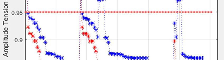
27                  Arouna Oloulade et al.: Contribution to the Economic and Optimal Planning of Multi-GED and a
                                      FACTS in a Distribution Network by Genetics Algorithms

balance of supply and demand and meet the requirements of           distribution network, that of Ouidah. It will be a question of
regulators which regulate the energy sector in several countries.   making a comparative study between the different possible
They are then subject to compliance with the most decisive          combinations of three GEDs (Wind generator (WG), PV and
performance criteria (stability, continuity of service, economy).   PAC) with the SVC, to bring out the best. This study will be
The constantly increasing charges, due to the demographic and       based not only on technical performance (reduction of energy
industrial growth of the countries, generate various                losses, improvement of the voltage profile, etc.), but also on
disturbances on the electrical network, in particular the losses    the environmental impact (reduction of gas emissions) and
of power, the drops in voltage and excessive Non Distributed        recovery of the energy saved. to ensure the profitability of the
Energies (END), recurrent triggers, dispersions of dangerous        project. For this, we will use the genetic algorithm of non-
potentials resulting from the poor flow of atmospheric              dominated sorting, the NSGA II, as an optimization tool.
discharges to the ground.
   Also, it is strong to note the incapacity of the conventional    2. Literature Review
means of voltage regulation (load regulators, capacitors,
phase shifting transformers, regulators of distribution                The optimal size and positioning are two key factors in the
transformers...) in distribution networks, to properly manage       integration of decentralized productions and FACTS into
the flows of loads, improve the bar voltage profiles and            existing electrical systems, and have become, in recent years,
increase the reliability of energy systems.                         real challenges and have been the subject of several studies.
   To remedy this, various effective approaches can be envisaged.   These studies, as diverse as they are, are generally based on
   One of these solutions is the decentralization of production     technical criteria (reduction of power or energy losses,
by Decentralized Energy Generators (GED). It makes it               improvement of the voltage profile, indices of network
possible to reduce the lengths of the lines for transporting        stability and performance, reduction of energy not distributed,
electrical energy, thereby reducing active and/or reactive          etc.), economic (reduction in investment cost, reduction in
losses on line. Among these GEDs, we can cite photovoltaic          upkeep and maintenance costs, profitability of the GED and
solar, wind generator, fuel cells, tidal power, biomass...          SVC placement project, etc.) and environmental (reduction
   However, decentralizing production is not always enough          of gas emissions, etc...) and use the multiple methods of
to effectively solve all the problems on the electrical             analysis and optimization available.
networks, especially in the event of high voltage instability.         One of the most used approaches for positioning and sizing
For example, the PVs fail to correct the voltage in the             GED is the analytical method. Thus, D. Q. Hung et al.
networks as much as the FACTS.                                      presented a methodology for the integration of distributed
   Taking advantage of the development of power electronics         (biomass) and non-dispatched (wind genrator) decentralized
which has introduced new devices called FACTS (Flexible             production units in renewable energy into electrical networks
Alternative Current Transmission System), network                   with a view to minimizing annual energy losses [2]. Analytical
managers are inserting them into the network to improve its         expressions are used to find the optimal size and power factor of
performance. FACTS enable more efficient operation of               the GED for each position in order to minimize power losses.
electrical networks by acting directly and continuously on the      These expressions are then adapted to place the GEDs for the
basic parameters of the networks, notably the phase shift,          minimization of the annual energy lost, taking into account the
voltage and impedance. Thus, they contribute to improving           temporal variation of demand and production. The method has
transit capacity, minimizing losses, improving voltage plans        been tested on the IEEE network 69 nodes for various scenarios
and increasing the operational flexibility of electrical               Besides the analytical methods, there are several other
networks. They act on the parameters both in stationary             approaches. Srinivas and Kale develop three positioning
regime and in transient regime. Among these devices, the            methods using respectively the PSO, the Modified Teaching
most used for networks with high voltage instability, are           Learning-Based Optimization algorithm (MTLBO) and the Jaya
shunt devices including the SVC (Static Var Compensator).           algorithm [3]. The goal is to reduce power losses and improve
   However, it is not enough just to place GEDs or FACTSs           voltage stability. They use the VSI. The different algorithms
[1]. Care must be taken to properly size them and find the          were tested on the IEEE 33 network and the results compared to
most optimal position possible in the distribution network.         those obtained with the conventional analytical method.
For this fact, we often use optimization methods, especially           ALO (Ant Lion Optimization) is also an optimization
meta-heuristics. The most commonly used are PSO (Particles          method used for the positioning of GEDs in the distribution
Swarm Optimization), ACO (Ant Colony Optimization) and              network. This is the approach used by Reddy P. et al. for the
GA (Genetic Algorithm). GAs are the most popular because            optimal positioning of GED types 1, 2 and 3. The approach is
of their efficiency and ease of implementation. We mainly           tested on IEEE 15, 33, 69 and 85 networks [4].
find SPEA (Strengh Pareto Evolutionary Algoritm) I and II,             Based on the PSO, Athira et al. [5] improved the technical
FastPGA (Fast Pareto Genetic Algorithm), NSGA (Non-                 performance of the distribution network by the simultaneous
dominated Sorting Genetic Algorithm) I and II.                      positioning of PAC and PV.
   Thus, in the present work, it will be a question of                 The FAMPSO (Fuzzy Adaptive Modified Particle Swarm
developing a power flow algorithm, and of optimizing the size       Optimization algorithm) was used to position a central
and the multi-GED positioning in the presence of the SVC in a       heating station in a distribution network and tested on the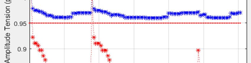
American Journal of Electrical Power and Energy Systems 2020; 9(2): 26-40                                       28

IEEE 69 network by Farjah et al. [6]. The objective function        Indonesian distribution network [14].
used involves the reduction of energy losses, the reduction of
gas emissions and the reduction of the voltage deviation.
   Minh Quan et al. used BBO (Biogeography-Based                    3. Calculation of the Electrical Condition
Optimization) to position PV in the network. Power losses,             of a Radial Distribution Network
THD (Total Harmonic Distortion) and IHD (Individual
Harmonic Distortion) are optimized technical performance               The calculation of the electrical state of an electrical
[7]. It is evaluated on the IEEE 33 and the IEEE 69. The            network involves the analysis of its power flow. Also called
comparisons made with the PSO, the ABC (Artificial Bee              “load distribution” or “load flow”, it is a basic tool and
Colony algorithm) and the GA allowed to conclude that this          necessary for any electrical system, and having for objective
approach is effective.                                              the determination of the various electrical variables (current
   The placement problem of SVC also requires the use of            in the lines, the voltage profile, power transits, line losses,
optimization methods and has been the subject of various studies.   etc.) at a given time, for a given state of consumption and
   Majid et al. used NSGA II for optimal placement of SVC           production. The general methods, namely Newton-Raphson,
and TCSC in the 30-node IEEE network [8].                           Gauss-Seidel, Scott and FDLF (Fast Decoupled Load Flow)
   Walaa et al. use probabilistic approaches for optimal            [15], converge well and are suitable for transport networks.
placement of the CVS. Several methods have been used and            However, they remain ineffective for the analysis of
compared in the context of their work. These are NSGA II,           distribution networks [16]. For these radial networks, the
MOPSO, PESA II and SPEA-2 [9]. The IEEE 33 and IEEE                 suitable methods are those based on the Backward and
69 networks are the test networks.                                  Forward Sweep (BFS) or double scanning, due to the low
   Mohamad Zamani et al. placed SVC in a network using the          X/R ratio of the distribution networks, the radial structure
Symbiotic Organism Search (SOS) algorithm [10]. The voltage         and the unbalanced load distribution [17].
deviation index was used to determine the position of the SVC.         The BFS variant used in this work is that of current and
Then, the SOS enabled the size of the SVC to be optimized.          voltage injection, based on the BIBC (Bus Injection to
   Studies have been carried out for the simultaneous               Branche Current) and BCBV (Branche Current to Bus
positioning of GED and SVC.                                         Voltage) matrix.
   Thus, Thishay and Balamurugan have developed a method            3.1. Mathematical Model of Network Elements
based on VSI for the positioning and dimensioning of SVC
and GED in a distribution network [11]. This approach has             Assuming the linear network with balanced steady-state
been tested on the IEEE network of 33 nodes                         operation [18], the study of the network can be carried out
   Rath and Ghatak addressed the problem of positioning GED         using an equivalent single-phase network presented at Figure 1.
and SVC using PSO [12]. This positioning was performed by a
combination of the PSO with the Rapid Voltage Stability Index
(FVSI) and the Line Stability Index (LQP). The contribution of
GED and or SVC was assessed by the voltage profile increase
index (VPII), the line loss reduction indices (ILP and ILQ) and          Figure 1. Single line diagram of a single power transmission line.
the net present value of the installation. This approach has been
tested on the IEEE 30 node and IEEE 12 node networks. Tests            In this model, the generators are considered as variable
have shown that GED has a considerable contribution in              voltage sources in series with an induction reactance (Figure
reducing losses compared to SVC.                                    2 (a)). In the p.u. system, this induction reactance is equal to
   Another very effective method of studying the integration        the unit, under normal conditions.
of GED into existing networks is the direct consideration of           The branches are represented by a resistor in series with an
the study of the profitability of the project in formulating the    inductive reactance (Figure 2 (b)). The line impedance is then
positioning problem. This consistent approach makes it              calculated by:
possible to satisfy both the technical performance of the
network, but also to ensure the profit margin for the network                                                  .                              (1)
manager, while respecting the environment. In this context,
                                                                      As for the loads, they are seen as consumers of active
Ali and Yang are based on the stochastic method of network
                                                                    power and reactive power (Figure 2 (c)). The apparent
planning, ADNP (Active Distribution Network Planning) for           power is then:
multi-GED positioning (Wind turbine + PV + Storage battery)
[13]. The objectives formulated are the minimization of                                                            .                          (2)
power losses, the rational exploitation of GEDs for the
satisfaction of demand, and the maximization of NPV (Net
Present Value). The approach is evaluated on the IEEE
network of 123 nodes and on a real network of 53 nodes.
   A similar approach was also used by Rodriguez-Gallegos                                 Figure 2. Single-line diagram.
et al. for the positioning of PV and Storage Batteries in an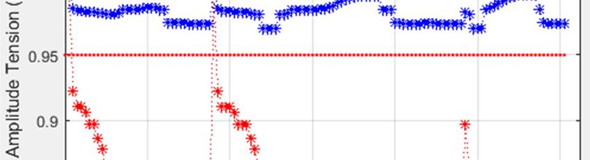
29                   Arouna Oloulade et al.: Contribution to the Economic and Optimal Planning of Multi-GED and a
                                       FACTS in a Distribution Network by Genetics Algorithms

3.2. Formation of BIBC and BCBV Matrices                                 2) Read tolerance ! (ε =0.00001).
                                                                         3) Read base voltage and power.
   The formulation of these two matrices is essentially based            Step 2:
on the topological data of the network. These are in particular          1) Formation of BIBC and BCBV matrices.
the number of nodes n, the number of branches b, the base                2) Initialization of iterations, " 1.
voltage , the base power , as well as the powers of the                  Step 3: Backward Sweep.
charges at the nodes and the characteristics of the lines.               1) Calculation of current injections at the different nodes
   The BIBC matrix:                                                         as follows:
   The BIBC matrix establishes the link between the current
                                                                                                                    $       ∗
injections of the load nodes and the currents of the different lines                                              # %'                                           (3)
   The approach allowing the construction of this matrix is                                                         &%

described by the Algorithm 1.                                            2) Calculation of branch currents by:
   Algorithm 1 Formation of the BIBC matrix
   Step 1: Create the × dimension matrix and initialize it to                                    )*+       )             +. ) +                                  (4)
zero. Each column represents a node, except the source node.
   Step 2: Set the first item to "1",      (1,1)      1.                 Step 4: Forward Sweep.
   Step 3: Either the branch , ≠ 1, between the nodes − 1                1) Calculation of the voltage drop by:
                                                                                    )∆ + = )             −        +=)                 +. )*+
and .
   a) Copy column − 1 from the BIBC matrix into column .                                             -                                                           (5)
   b) Set the     element of the line to 1.                              2) Calculation of new nodal voltages, .                          (/0 )
                                                                                                                                                  1 by:
   Step 4: Repeat the previous steps for all branches of the
network.                                                                                         ) + = ) - + − )∆ +                                              (6)

    The matrix obtained is an upper triangular matrix,                   Step 5: Assessment of the stopping criterion.
containing only 0 and 1.                                                 Calculate the maximum difference between the values of
    The BCBV matrix:                                                   nodal voltages of two consecutive iterations:

                                                                                        2345 = 6 78.                    (/0 )
                                                                                                                                 1−.      (/)
                                                                                                                                                19
    This matrix is the ratio between the branch currents and
                                                                                                                                                                 (7)
the nodal voltages. The process of its formation is described
by the Algorithm 2.                                                      1) Check if the maximum deviation is below the tolerance
    Algorithm 2 Formation of the BCBV matrix                                (2345 < !).
    Step 1: Create the matrix of dimension × and initialize              2) If yes, go to Step 6.
it to zero. Each line represents a node, except the source node.         3) If not:
    Step 2: Set the first item to " ",       (1,1)        .                 a) go to the next iteration, " = " + 1.
    Step 3: Either the branch , ≠ 1, between the nodes − 1                  b) back to Step 3.
and .                                                                    Step 6: Calculate the VSI at each node, by:
    a) Copy line − 1 from the BCBV matrix into line .
    b) Set the    element of the line to .                                         0    = | |< − 4 ∗ (                  0  .     0    − 0 .             0   )> − 4 ∗
    Step 4: Repeat the previous steps for all branches of the                            ( 0 . 0 +                       0 .      0   ) ∗ | |<                   (8)
network.
                                                                         Step 7: Perform the power balance.
  The matrix obtained is a lower triangular matrix,                      1) Total active loss:

                                                                                            = ∑DE                   = ∑DE               ∗ |* |>
containing only 0 and .
                                                                                  ?.@ABB                   @ABB,                                                 (9)
3.3. Algorithm of BIBC/BCBV Method
                                                                         2) Total reactive loss:
   The power flow method developed in this work finds its
simplicity in the exploitation of Kirchhoff's laws. It is based                         ?.@ABB   = ∑DE             @ABB,        = ∑DE          ∗ |* |>         (10)
on the structure of radial electrical distribution networks. It
                                                                         3) Powers of the source node:
uses the BIBC and BCBV matrices, while implementing the
principle of double scanning.                                                   B@4F/   =    G   +       ?.@ABB    = ∑4E              +    ?.@ABB               (11)
   The stages of power flow by the method based on the
matrices BIBC and BCBV, are described by the Algorithm 3.                       B@4F/   =    G   +       ?.@ABB    = ∑4E              +        ?.@ABB          (12)
   Algorithm 3 Power flow by the BIBC/BCBV method
                                                                         Step 8: Show power flow solutions.
   Step 1:
   1) Read network data:                                               3.4. Power Flow Results
      a) Number of nodes;
      b) Number of branches;                                           3.4.1. IEEE 69 Nodes Network
      c) Characteristics of the lines;                                   The validation of the developed power flow method is
      d) Information on the charges at each node.                      done on the IEEE 69 standard network, the structure of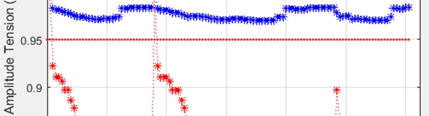
American Journal of Electrical Power and Energy Systems 2020; 9(2): 26-40                                        30

which is presented at Figure 3.
   This network has a voltage level of 12.66 kV and its data
is taken from [19].

                                                                                        Figure 4. Voltage profile of the IEEE network 69 nodes.

             Figure 3. Diagram of the 69-node IEEE network.                    The summary of the comparison is entered in the Table 1.
                                                                               Analysis of the results in Table 1 shows that the voltages
  This network is simulated with the algorithm developed in                  obtained by the method developed are almost identical to
MATLAB and the results obtained have been compared to                        those of the reference. Also, the deviations obtained are
those of Pedanna and Rama [20].                                              within the admissible ranges.
  The voltage profile is shown at Figure 4.
                                               Table 1. Comparison of test results on the IEEE 69 nodes.

 Parameters                                Sophisticated method                    Reference                     Relative deviation (%)
 Number of unstable nodes                  9                                       9                             0
 Minimum voltage                           0.90338 p.u. (64)                       0.90930 p.u. (64)             0.65
 VSI                                       0.66594 p.u. (65)                       -                             -
 Total active loss (kW)                    238.6699                                224.8799                      6.13
 Total reactive loss (kVAr)                106.9868                                102.1091                      4.77

   In view of these results, the current and voltage injection
algorithm, based on the BIBC and BCBV matrices,
developed in MATLAB, can be validated and applied to real
networks.

3.4.2. Ouidah MV Distribution Network
   The HVA departures of Ouidah are located in the
commune of Ouidah. This network originates at the 161
kV/20 kV Avakpa transformer station located in the DRA.
The Avakpa transformer station supplies two departures
(Ouidah and Allada) and takes its source on the L225-161 kV
line from Maria-Gléta and Momé Hagou. This network has
122 nodes, with a radial structure presented to The HTA
departure from Ouidah is located in the commune of Ouidah.
This network originates at the 161 kV/20 kV Avakpa
transformer station located in the DRA. The Avakpa
transformer station supplies two departures (Ouidah and
Allada) and takes its source on the L225-161 kV line from
Maria-Gléta and Momé Hagou. This network has 122 nodes,
with a radial structure presented at Figure 5.
   The simulation of this SBEE network with the elaborate
power flow method made it possible to obtain the voltage and
VSI profiles presented at the Figures 6 and 7.

                                                                                                Figure 5. Ouidah network architecture.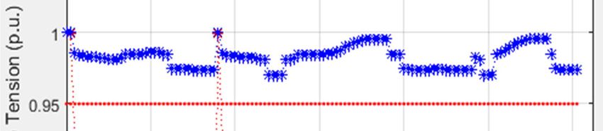
31                  Arouna Oloulade et al.: Contribution to the Economic and Optimal Planning of Multi-GED and a
                                      FACTS in a Distribution Network by Genetics Algorithms

                                                                    4. Formulation of the Problem of Size
                                                                       and Positioning of Multi-GED and
                                                                       SVC
                                                                    4.1. GED Modeling

                                                                       A Decentralized Energy Generator (GED) is any energy
                                                                    source connected to the transport, distribution or distribution
                                                                    network and which is part of unconventional (wind, solar
                                                                    photovoltaic, fuel cell, etc.) or conventional energies. small
                                                                    power, power less than 200 MW (gas micro-turbines,
                                                                    cogeneration, means of energy storage among others),
                                                                    outside large power plants. Their main advantages are: their
                                                                    short installation time (up to less than six months), their low
                                                                    investment and maintenance cost, the reduction of line losses,
                                                                    the improvement of the voltage profile, the reduction of toxic
              Figure 6. Ouidah network voltage profile.
                                                                    gas emissions and increased energy efficiency and network
                                                                    reliability.
                                                                       As part of our study, we opted for Type 1 GEDs (capable
                                                                    of providing active power only) and Type 3 (capable of
                                                                    providing active power and reactive power). For Type 1, we
                                                                    take the case of photovoltaic solar (due to the high solar
                                                                    potential available to Benin, with an average sunshine of 3.9
                                                                    kWh/m3 [22]) and that of fuel cells. Regarding Type 3, it will
                                                                    be the variable speed wind turbine, in particular that based on
                                                                    MADA (Asynchronous Dual Power Machine), because of the
                                                                    coastal edge available to Ouidah and the wind speed between
                                                                    4 and 6 m/s.
                                                                       The choice of GED type 1 is made because of their ability
                                                                    to provide active power. The latter is necessary in our study
                                                                    to influence the power transit and thereby reduce losses. As
                                                                    for GED type 3, it is not only the supply of active power but
                                                                    also its ability to provide reactive power when needed.
                                                                       GEDs are integrated into electrical networks to provide or
                Figure 7. Ouidah network VSI profile.               absorb active or reactive power or both. Thus, whatever the
                                                                    type of GED, they are considered as sources of active and/or
   From the analysis of these results, it appears that out of the   reactive power (positive or negative, depending on the type).
122 nodes of the network, only three (03) have amplitudes              A GED placed in node i is then represented as shown at
conforming to the NF 15160 and IEEE Standard 1860-2014              Fihure 8.
standards which stipulate that the nodal voltages must be in
the proportions of ± 5% of the nominal value, i.e. 0.95 pu at
1.05 p.u., so that the receivers are properly powered, so this
network has 119 unstable nodes, with a minimum voltage of
0.80455 p.u. at node 86. The minimum VSI is then 0.41897
p.u. at node 87.                                                                  Figure 8. Connection of a GED to node i.
   In terms of losses, the power losses are 457.34588 kW
(active losses) and 625.41503 kVAr (reactive losses). These           With this integration, the power injection at the node
losses represent respectively a rate of 13.45% of the total         changes. In the presence of the GED, the new active and
active power generated and 30.21% of the total reactive             reactive powers consumed at this node are then:

                                                                                                ,IJK            LMN
power generated. These rates do not comply with the
                                                                                            H
                                                                                                ,IJK             LMN
tolerance for allowed power losses. Indeed, for distribution                                                                  (13)
networks, power losses must be between 3% and 5% [21].
   From various analyzes, it appears that the network of                     ,   : PQT P U VP WT X YT VP WT Z[OTY\ [] PQT U[ X
                                                                    O PQ R   LMN , LMN PQT VP WT      X YT VP WT Z[OTY\ [] PQT ^_2
                                                                               ,IJK , ,IJK : PQT TO Z[OTY\ V[ \`6TX P PQT [XT
Ouidah is sinister, with excessive losses and a high instability
in voltage.

                                                                      Note that there is a relationship of dependence between the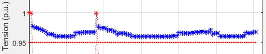
American Journal of Electrical Power and Energy Systems 2020; 9(2): 26-40                                       32

                                                                                                                y
                                                                                                                           gstu
                                                                                                                         gz{|,stu
active and reactive powers of the GED. Indeed, the reactive                                                                                         (23)
power is given by:
                                    ∗ LMN                                          a) if y : 0,05 then x 0,2716
                                                                                                          y • 0,05
                               LMN
                  a
                                                                                      x 0,9030. y „ 2,999. y < 3,6503. y …
                          b tan8 YVV[\( fLMN )9
                                                                         (14)      b) if                                               then

4.1.1. PV Modeling                                                                    2,0740. y > 0,4623. y         0,3747
   PV being a GED of Type 1, it is modeled like a source                           The annual cost of upkeep and maintenance is assessed as
(injection) of active power g& only. When it is placed in a                     follows:
node i, the power in this node becomes:
                                                                                          3,gop       i3,gop . qr O PQ i3,gop             $/Q       (24)
                                ,IJK              g&                     (15)
                                                                                ammonia oxide †‡5 and sulfur dioxide ‡> . The total gas
                                                                                  Fuel cells, during their operation, emit gases such as

modification because g& 0.
   The reactive power of the node does not undergo any
                                                                                emission is given by:
   Depending on the power of the PV to be installed, the                           _gop    qr .   gop . 8Tˆ‰|       T$‰Š 9 O PQ Tˆ‰| , T$‰Š   w/"lQ (25)
investment cost (purchase and installation) is determined as
follows:                                                                        4.2. SVC Modeling

        IB ,g&    i IB    ,g& . g&     O PQ i IB       ,g&     $/"l      (16)      The SVC (Static Var Compensator, i.e. static reactive
                                                                                power compensator), is a FACTS shunt device used in
  As for the annual cost of maintenance of the photovoltaic                     electrical networks to provide or absorb reactive power, in
power plant, it is assessed as follows:                                         order to act on network parameters, in particular the voltage
      3,g&     i3,g& .    g&   O PQ i3,g&              $/"l/mY           (17)   profile.
                                                                                   It is a group of parallel capacitors and inductors, with a
4.1.2. Wind Generator Model                                                     fairly rapid control action, thanks to the switching of the
  The Wind Generator used in this work is based on a                            thyristors or mechanically [23]. It is then generally
MADA. It is therefore a GED of Type 3. Therefore, it is                         represented by a combination of TSC-TCR (Thyristor
modeled as a source (injection) of active powers nL and                         Switched Capacitor - TCR).
reactive nL . When placed in a node i, the powers in this                          The SVC is connected to the network via a coupling
node become:                                                                    transformer ensuring the filtering of the harmonic currents

                      H
                          ,IJK                 nL
                                                                                resulting from the delay angle of the thyristors and from the
                          ,IJK                  nL
                                                                         (18)   resonance due to the presence of the capacitors.
                                                                                   It is considered as a variable parallel reactance (Figure 9),
  The cost necessary for the installation of this wind power                    which is adjusted in response to the operating conditions of
plant is given by:                                                              the electrical network in order to control its parameters,

                   i IB   ,nL . nL       O PQ i IB               $/"l (19)
                                                                                specifically the voltage.
        IB ,nL                                           ,nL                       Depending on the reactance (inductive or capacitive), the
                                                                                SVC is capable of drawing a capacitive or inductive current
    As for the annual maintenance cost of a wind power plant,
                                                                                from the network, at the point of its coupling. Perfect control
it is assessed as follows:
                                                                                of this equivalent reactance makes it possible to regulate the
        3,nL      i3,nL .       nL     O PQ i3,nL             $/"l/mY    (20)   voltage module at the SVC connection node, and therefore
                                                                                have a direct impact on the network voltage profile.
4.1.3. Fuel Cell (FC or PAC) Modeling
    PACs are active power gop sources only. Placed in a node
i, the active power injection in the latter becomes:

                               ,IJK              gop                     (21)

  The necessary investment is:

                                  i IB   ,gop . qr .
                                                       gstu
                  IB ,gop                               v
                                                                         (22)

                               i IB ,gop $/"lQ
     O PQ Rqr : PQT            ` U [ZTY P w P 6T                 Q[`Y\
                                  x: PQT m TUX
                                                                                           Figure 9. SVC variable shunt susceptance model.

                                                                                  Connected at a node , the current that the SVC absorbs is
   The efficiency is calculated according to the ratio between
                                                                                given by:
the power of the FC and the maximum power. We define: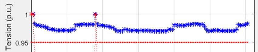
33 Arouna Oloulade et al.: Contribution to the Economic and Optimal Planning of Multi-GED and a
FACTS in a Distribution Network by Genetics Algorithms
$&p . $&p . (26) ensure that the project is economically profitable and feasible.
We will discuss here, minimizing the return on investment
Depending on this current, the power of the installed SVC period (PRI) and maximizing the net present value (NPV).
is determined, by: 1) The return on investment period:
$&p = . $&p . =− $&p .
>
(27) It is a financial indicator that measures the time between
investment and the cumulative recovery of invested capital.
Thus, the power injected into this neoud is modified as In other words, it is the time it takes for the cumulative
follows: revenue to balance the initial investment. PRI is determined
= −
with the following formula:
,IJK $&p (28)
p%Ž•.%Ž%
]< = = (35)
The investment necessary for the installation of such a •Ž‘’’‘
system is given by [24]: With:
IB ,$&p = 0,0003. >
$&p − 0,3051. $&p + 127,38 (29) Ir. I = PP U WT\P6T P = IB + J “GJ
$&p is in kVAr and IB ,$&p in dollars $. IB = \P UU P [ V[\P
The cost of annual maintenance is given by:
J “GJ = \P`Xm V[\P\ = 0,2 ∗ IB
3,$&p = 0,05 ∗ IB ,$&p (30)
IJ J = ` U TP YTWT `T = 4I − 3
= ` U6 PT VT V[\P\
4.3. The Objective Functions
3
= ` U YTWT `T = iM . _B4rJ
4.3.1. Technical Performance
The almost permanent satisfaction of the demand and the 4I
respect of the margins of security and stability of the network, iM = WTY wT V[\P [] "lℎ P __
are the determining elements in term of performance of an
electrical system. To contribute to this, the performances _B4rJ = ` U T TYwm \ WTX _B4rJ
taken into account in this work concern the minimization of = qr ∗ # ?.@ABB{•{Ž’ − ?.@ABB{”•è— '
energy losses in lines and the minimization of deviation in
expansion. 2) The net present value:
1) Lost energy: The net present value (NPV) of an investment is the
The energy lost is the energy loss induced by power losses. difference between the net present gains of the investment
Its reduction includes not only that of power losses, but also (inflows minus outflows) and the starting bet. The investment
is related, in some way, to the reduction of undistributed will be profitable if this result is positive. It is calculated as
energy. The annual active and reactive energies lost, are follows:
−
expressed by:
4I Ir
˜† =
] = U[\P VP WT T TYwm = qr . ?.@ABB (31) fF™š
]> = U[\P YT VP WT T TYwm = qr . ?.@ABB (32) ]„ = (36)
&oˆ
O ith qr = q − qF OℎTYT qF \ PℎT ` U V`P − []] P 6T
2) Voltage deviation: With:
It expresses the relative difference between the nodal X. (1 + X) ”
fF™š = YTP`Y [ WT\P6T P ] VP[Y =
(1 + X) ” − 1
tension and the specific reference tension. The reduction of
this factor will make it possible to bring back the nodal
voltages within the limits of admissible voltages fixed by X = X \V[` P Y PT
the standards in force. It is given by:
P› = ZY[ TVP U ]T X`Y P [
|&Œ |•|&% |
]… = W[UP wT XTW P [ = 6 7 # |&Œ |
' (33)
Ir = P[P U WT\P6T P V[\P
= . fF™š + 3 + ™ . fBBš (X, PF )
In our work, technical performance is brought together in
Ir Ir. I
an aggregative function. This function groups together the P™
− ™ . . fBšš 8X, P› 9
PF
active and reactive energies lost, and the voltage deviation.
We have:
= V[\P [] YTZU V w Tœ` Z6T P
f = 0,4 ∗ ] + 0,3 ∗ ]> + 0,3 ∗ ]… (34) ™
PF = U ]TP 6T [] Tœ` Z6T P
4.3.2. The Economic Criterion
Taking this criterion into account makes it possible to P™ = YT\ X` U \TYW VT U ]T [] Tœ` Z6T P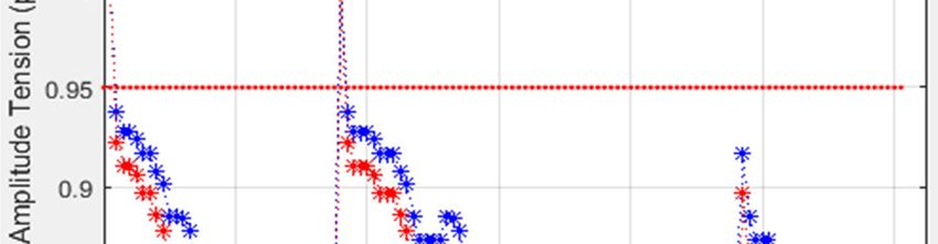
American Journal of Electrical Power and Energy Systems 2020; 9(2): 26-40 34
fBšš U[\\ ] VP[Y susceptances.
X
4) PV penetration rate:
fBBš (X, PF ) The penetration rate is the ratio of the active power of the
(1 X) • − 1 PV plant installed on the total demand of the network. This
X PV penetration rate in a distribution network must not exceed
fBBš 8X, P› 9
(1 X) −1
”
30% of total demand in order not to disturb the network
protection equipment. This constraint is formulated as
4.3.3. The Environmental Criterion follows:
≤ 0.3 ∗
This criterion consists in minimizing gas emissions. It is
g& G (44)
expressed by the function:
]ž _gop
5) Constraint related to profitability:
(37)
A project is profitable when its net present value is positive.
In this work, the economic (profitability) and So, this constraint is formulated as follows:
˜† > 0
environmental (reduction of gas emissions) aspects have
(45)
been combined into a single objective function. This function
is defined as follows: 4.5. Adaptation of the NSGA II to the Problem of Size and
0,4. ]< + 0,6 ∗ ]„ , ] ]ž = 0
Positioning Multi-GED in the Presence of the SVC
f> H
0,3 ∗ ]< + 0,4 ∗ ]„ + 0,3 ∗ ]ž , ] ]ž ≠ 0
(38)
The NSGA (Non-dominated Sorting Genetic Algorithm) II
is an elitist Pareto genetic method, ie it uses the concept of
4.4. Constraints
Pareto dominance to perform a quick sorting, an
The resolution of any optimization problem must be done overcrowding distance to ensure the divesity of the solutions
under certain constraints. For the placement of GED and in the same front and keeps Pareto-optimal solutions for
SVC, these constraints relate to the conditions of operation of reintroduction in new populations.
the network and the standards in force. The optimization method based on the NSGA II is
presented by algorithm 4.
4.4.1. Equality Constraints Algorithm 4 Multi-GED optimization in the presence of
The equality constraints concern the balance of the SVC, with NSGA II
network, in the presence of GEDs and SVCs. We have: Step 1: Read data.
I
+ ∑ EŸ = +
¡ a) Network data.
B@4F/ LMN G ?.@ABB (39)
b) Parameters of NSGA-II, SVC and GED.
B@4F/
I
+ ∑ EŸ ¡
LMN + $&p = G + ?.@ABB (40) Step 2: Generate initial population - = ¤7 , 7> , … , 7ˆ”¦” §
taking into account the information read in Step 1 then set the
4.4.2. Inequality Constraints generation counter to zero (P = 0).
1) Constraints related to voltage: With †›A› the number of individuals in the population and
This constraint makes it possible to maintain the nodal the 7 are the decision variables (positions and sizes of the
voltages in the range of admissible values. We have: various GED and SVC).
3I ≤ ≤ 345 (41) Step 3: For each individual in the population , run the
power flow using the BIBC/BCBV algorithm and evaluate
3I = 0,95 Z. `. , PℎT 6 6`6 X6 \\ UT W[UP wT
O Pℎ H the objective functions.
345 = 1,05 Z. `. , PℎT 6 7 6`6 X6 \\ UT W[UP wT Step 4: Check the constraints and add the penalty to the
objective functions of the individuals who violated the
2) Constraint related to the capacity of GEDs:
constraints.
The GEDs to be installed must have limited capacities, to Step 5: Generate the population of children from by
ensure the balance of the system. We have: applying genetic operators (crossing and mutation) to obtain
3I
≤ ≤ 345 the intermediate population = ∪ with size 2 ∗ †›A› .
LMN LMN LMN (42)
Step 6: Classify the population by fronts (using the
3I 345
With LMN et LMN , the minimum and maximum active power flow).
powers of GED . Step: Select †›A› individuals from the 2 ∗ †›A› to form
3) Constraint related to the capacity of the SVC: the population 0 .
The SVC installed must have limited capacity. We have: Step 8: Increment the generation counter (P = P + 1) and
repeat steps 3 to 7 until the total number of generations is
3I
$&p ≤ $&p ≤ 345
$&p (43) reached.
$&p = − 3 I . $&p
3I > 345 Step: Take out the optimal solutions in the sense of Pareto
With a and choose the best solution.
$&p = − 345 . $&p
345 > 3I
3I 345 The parameters used are listed in Table 2.
With $&p et $&p , SVC’s minimum and maximum shunt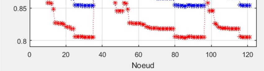
35 Arouna Oloulade et al.: Contribution to the Economic and Optimal Planning of Multi-GED and a
FACTS in a Distribution Network by Genetics Algorithms
Table 2. NSGA II simulation parameters. positioning of PV and PAC separately.
Parameters Values
5.1.2. Multi-GED Optimization: Case of PV + PAC
Population size 100
Number of generations 150
Execution of the optimization algorithm places a 100 kW
Probability of crossing 0,9
Probability of mutation 0,2 PV central at node 121 and the 578 kW PAC at node 92.
Number of function-objective 02 This integration requires 432,229,782.6 CFA francs and
Number of variables 02 to 08 ensures a reduction in active and reactive losses of 41.42%
Number of constraints 04 to 06 and 41.49% respectively. This reduction in losses is better
than those obtained with each GED separately. However, the
5. Results and Discussions impact on the stress plane is still not interesting. The
minimum value of the VSI is 0.51180 p.u. As for the tension,
As part of this work, various combinations between GED its minimum value is 0.94582 p.u. and is obtained at node 86.
(PV, PAC, Wind turbine) and SVC were studied. The number of unstable nodes is 119 (Figure 11).
5.1. Optimization of GED Alone
Here, we present the results from the optimization of sizes
and positions of GED only in the network.
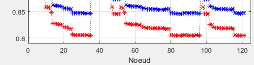
5.1.1. Mono-GED Optimization: Wind Turbine Case
After running the optimization algorithm based on the
NSGA II, we obtained a population of solutions from which
we chose the best. Thus, it will be necessary to install a 905
kW wind power plant at node 50 of the Ouidah network.
The integration of this plant reduces active and reactive
losses by 34.39% and 38.14% respectively, bringing them to
300.06341 kW and 386.83065 kVAr. However, there are still
112 unstable nodes in the network (Figure 10). This project
requires an initial investment of 1,173,174,344 CFA francs
and the return on investment will be made after 10 years,
approximately 18 days.
The minimum voltage value is 0.85339 p.u. This voltage Figure 11. Voltage profile in the presence of PV and PAC.
value is always lower than the minimum admissible value
To remedy the problem of the stress plane, it is then
(0.95 p.u.). In addition, instability is also confirmed by the
necessary to find an effective solution. The most suitable
values of the VSI, the minimum value of which is 0.53037.
solution is the installation of a FACTS shunt type device,
Figure 10 presents the voltage profile in the presence of
here the SVC.
the wind turbine.
5.2. Optimization of SVC Alone
Optimizing the size and position of the SVC leads to the
installation of a 3,523 MVAr SVC at node 72 of the Ouidah
network.
The cost of installation is 1,656,338,617 CFA francs, with
a return on investment spread over approximately 5 months
and 18 days.
With this integration, the voltage profile and the voltage
stability are significantly improved. Indeed, it is noted that all
the voltages are brought back within the range of admissible
values. Thus, the minimum voltage value goes from 0.80455
p.u. to 0.97033 p.u., an increase of 20.60%. Likewise, the
minimum value of VSI goes from 0.41897 p.u. at 0.88651
p.u., an increase of 11.59%. The tension profile is shown in
Figure 12.
Figure 10. Voltage profile in the presence of the wind turbine.
There is certainly a slight improvement in stability, given
this figure, but this improvement is not satisfactory.
The same observation was made for the single-GEDAmerican Journal of Electrical Power and Energy Systems 2020; 9(2): 26-40 36
Figure 12. Voltage profile in the presence of SVC. Figure 14. VSI profile with PV, PAC and SVC.
In addition, we note that the SVC does not really manage With these positioning, the active and reactive losses were
to influence the power transit in view of the reduction of reduced by 42.19% and 42.16%, thus passing to 264.37152
losses. It only reduces active losses by 0.89% and reactive kW and 361.73704 kVAr respectively. This reduction
losses by 2.43%. increases the availability of electrical energy at the customer
level and increases the profit margin of SBEE. This project
5.3. Multi-GED Optimization in the Presence of SVC will be installed at a cost of 439,350,784.9 CFA francs with a
In view of the previous results and analyzes, it is argued return on investment spread over 8 years 5 months and 27
that taken separately, the GEDs and the SVC fail to resolve days approximately.
both the loss and voltage stability problems, while increasing 5.3.2. Project 2: PV + Wind Turbine + SVC
the profit margin of the SBEE. Thus, the most likely solution The execution of the optimization algorithm gives a central
is the combination of GED and SVC. It will then be question, PV of 0.2 MW at node 99, a wind power plant of 0.684 MW
here, to present the results from multi-GED optimizations in at node 32 and an SVC of 1.955 MVAr at node 28. The
the presence of the SVC in the Ouidah network. results are presented in Table 3. The voltage and VSI profiles
5.3.1. Project 1: PV + PAC + SVC obtained are shown in Figures 15 and 16.
The optimization carried out allowed us to place a PV of
200 kW, a PAC system of 282 kW and a SVC of 2,438 MVAr
respectively at nodes 51, 74 and 94 of the Ouidah network.
This integration contributes to a 100% reduction in the
number of unstable nodes, with a minimum tension of
0.96017 p.u. at node 76 (Table 3). There is also a significant
improvement in terms of voltage stability, with a minimum
VSI of 0.84997 p.u. The tension profile is shown in Figure 13.
Figure 15. Voltage profile with PV, Wind turbine and SVC.
In these figures, there is a significant difference between
the profiles before and after optimization. After optimization,
all voltages are in the admissible value range. The minimum
voltage value is then 0.97002 p.u. Voltage stability has also
Figure 13. Voltage profile with PV, PAC and SVC. improved, with a minimum value of VSI increasing from37 Arouna Oloulade et al.: Contribution to the Economic and Optimal Planning of Multi-GED and a
FACTS in a Distribution Network by Genetics Algorithms
0.41897 p.u. at 0.88366 p.u. There is also a reduction of the range of admissible values. Thus, the minimum tension
61.05% in active line losses. This reduction results in a net found is 0.95993 p.u. (Figure 17). This voltage stability is
annual gain of 211,921,991.6 CFA francs. This ensures a confirmed by the values of the VSI. The lowest VSI is then
recovery of the funds invested after 5 years 7 months and 14 0.84909 p.u. (Figure 18).
days approximately.
Figure 18. VSI profile in the presence of PAC, wind turbine and SVC.
Figure 16. VSI profile with PV, Wind turbine and SVC.
5.3.4. Project 4: PV + PAC + Wind Turbine + SVC
5.3.3. Project 3: PAC + Wind Turbine + SVC With regard to the positioning of the three GEDs and the
For this combination, the solution chosen is that of the SVC, the execution of the optimization algorithm places a
placement of a 200 kW Pac system at node 51, a 318 kW central PV of 0.131 MW at node 51, a wind turbine of 121
wind turbine at node 74 and a 2,217 MVAr SVC at node 93 kW at node 75, a Pac system of 700 kW at node 34 and a
of the Ouidah network (Table 3). The installation of these SVC of 2.126 MVAr at node 93.
systems requires 505,551,789.2 CFA francs. The return on This multi-GED integration in the presence of the SVC
investment will be made after - years 2 months and 27 days ensures a reduction of 65.12% in active losses and 65.11% in
approximately. reactive losses. This reduction allows recovery of the funds
With the placement of these two GEDs and SVc, the state invested after 4 years 6 months and 4 days approximately.
of the network is improved, with a 45.44% reduction in From the voltage point of view, all the nodes are stable. The
active losses. As for reactive losses, they go from 625.41503 minimum voltage being 0.96993 p.u., or 19.3986 kV. The
kVAr to 341.40405 kVAr. minimum VSI is then 0.88505 p.u. These profiles are shown
in Figures 19 and 20.
Figure 17. Voltage profile in the presence of PAC, wind turbine and SVC.
Figure 19. Voltage profile in the presence of PV, Fuel Cell, Wind turbine and
We note the absence of unstable nodes in the network. SVC.
Indeed, after optimization, we note that all the voltages are inAmerican Journal of Electrical Power and Energy Systems 2020; 9(2): 26-40 38
Table 3. Summary of multi-GED optimizations in the presence of SVC.
Project 1 Project 2 Project 3 Project 4
Parameters Before optimization
PV + PAC + SVC PV + WG + SVC PAC + WG + SVC 3 GED + SVC
PV (kW) - 200/51 200/99 - 131/51
PAC (kW) - 282/74 - 200/51 700/34
WG (kW) - - 684/32 318/74 121/75
SVC (MVAr) - 2.438/94 1.955/28 2.217/93 2.126/94
IB (F CFA) - 439,350,784.9 1,168,039,710 505,551,789.2 693,482,704.6
3 (F CFA/yr) - 103,522,086.3 26,322,619.14 105,909,924.4 104,661,816.1
_gop (g/yr) - 92,328.209 - 65,481 229,183.5
3 I (p.u.) 0.80455/86 0.96017/76 0.97002/76 0.95993/109 0.96993/76
Unstable nodes 119 0 0 0 0
3 I (p.u.) 0.41897/87 0.84997/77 0.88536/77 0.84909/110 0.88505/77
?.@ABB (kW) 457.34588 26437152 178.12310 249.49970 159.48801
Reduction of ?.@ABB - 42.19% 61.05% 45.44% 65.12%
?.@ABB (kVAr) 625.41503 361.73704 243.41500 341.40405 218.16875
Reduction of ?.@ABB - 42.16% 61.05% 45.41% 65.11%
_B4rJ (kWh/yr) - 1 446 687.491 2 205 137.816 1 744 868.659 2 411 239.843
IJ J (F CFA /yr) - 52 779 027.8 211 921 991.6 82 606 889.27 155 850 200.4
PRI (years) - 8.491 5.622 6.242 4.539
VAN (F CFA) - 63 827 318.57 1 556 350 848 350 326 219.9 999 126 776.6
1) for active losses, the first row is reserved for the
solution giving less power losses, that is to say that
offering a good reduction in active losses;
2) for the other five criteria, the first row is reserved for
the solution with the highest value.
Then, depending on the total weight of each combination,
we assign a rank for the classification. Thus, the solution that
best adapts is the one with the lowest weight.
The results of this classification are presented in Table 4.
Table 4. Ranking of the best solutions.
Criterion Project 1 Project 2 Project 3 Project 4
IB 1 4 2 3
PRI 4 2 3 1
VAN 4 1 3 2
3I 3 1 4 2
3I 3 1 4 2
?.@ABB 4 2 3 1
Figure 20. VSI profile in the presence of PV, Fuel Cell, Wind turbine and Poids total 19 11 19 11
SVC.
At the end of this classification, we obtain two better
5.4. Choosing the Best Solution solutions instead of one. These two solutions have the same
weight (11). These are the PV + Wind turbine + SVC and PV
In view of the results presented in the previous section, we + PAC + Wind turbine + SVC combinations.
note that only multi-GED combinations in the presence of To get the best out of it, we base ourselves on the
CVS manage to meet both technical, environmental and installation cost and the active losses. On this basis, we note
economic expectations. These combinations are all effective that the last combination (PV + PAC + Wind turbine + SVC)
and profitable, a choice is necessary. In order to choose the is better, because it is less expensive and with a high
best solution among these four combinations, a selection reduction rate of active losses.
method is adopted. Thus, at the end of this work, the suitable solution for
We proceed to a classification. For this, six criteria are improving the technical performance of the Ouidah network
taken into account, namely: installation cost, return on and increasing the profit margin of the SBEE is the
investment period, NPV, minimum voltage, minimum VSI integration of three GEDs (PV, PAC and wind turbine) and an
and active losses. SVC. These are the positioning of a 121 kW wind turbine, a
This classification will be done by weighting the 131 kW photovoltaic power plant, a 700 kW PAC system and
parameters mentioned. Indeed, for each of these criteria, the a SVC of 2.126 MVAr, respectively at nodes 75, 51, 34 and
solutions are classified according to their rank. The rank 94 of the Ouidah MV network. This project requires an initial
corresponds to the weight. This classification is done as investment of 707,352,358.7 CFA francs.
follows:39 Arouna Oloulade et al.: Contribution to the Economic and Optimal Planning of Multi-GED and a
FACTS in a Distribution Network by Genetics Algorithms
This investment will be recovered after 4 years 6 months Generation Units in Radial Distribution Systems», Energies
and 14 days approximately, thanks to a net annual income of 2019, 12, 174.
155,850,200.4 CFA francs. [8] Majid Aryanezhad, Elahe Ostadaghaee, Mahmood Joorabian,
«Optimal Allocation and sizing of FACTS Devices Based
Non-dominated Sorting Genetic Algorithm II», The 1st Iran
6. Conclusion Energy Association National Conference - 2013 Tehran, No.
13-EN-EPP-1242.
In this work, the proposed power flow method was tested
on a standard 69 node network and on a real 122 node [9] Walaa Ahmed, Ali Selim, Salah Kamel, Juan Yu, Francisco
network of the SBEE. This method confirmed the state of the Jurado, «Probabilistic Load Flow Solution Considering
Optimal Allocation of SVC in Radial Distribution System»,
Ouidah distribution network, with excessive losses and high International Journal of Interactive Multimedia and Artificial
voltage insatability. To remedy this, a method for optimizing Intelligence, Vol. 5, No. 3.
sizes and multi-GED positioning in the presence of SVC,
[10] Mohamad Khairuzzaman Mohamad Zamani, Ismail Musirin,
based on the NSGA II, was proposed. With these methods,
and Saiful Izwan Suliman, «Symbiotic Organisms Search
various combinations were studied and the application of a Technique for SVC Installation in Voltage Control»,
selection by weighting made it possible to choose the optimal Indonesian Journal of Electrical Engineering and Computer
solution among the best. From the results obtained, it appears Science, 6 (2): 318, May 2017.
that the optimization of sizes and multi-GED and SVC [11] Thishya Varshitha U., Balamurugan K., «Optimal placement
positions, with direct consideration of economic profitability, of distibuted generation with SVC for power loss reduction in
in a distribution network, contributes to the significant distributed system», ARPN Journal of Engineering and
reduction of energy losses in lines, the improvement of the Applied Sciences, Vol. 1, No. 17, September 2017.
voltage profile and stability, as well as an increase in the [12] A. Rath, S Roy Ghatak, «Technical and Economic Assessment
manager's profit margin. This project has a very interesting of Power System by Incorporating Distributed Generation and
benefit-cost ratio and may well be the subject of a detailed Static VAR Compensator», Smart Grid, 3 (1): 6, 2016.
financial study to serve as decision-making tools for donors. [13] Ali Ehsan, Qiang Yang, “Coordinated Investment Planning of
Distributed Multi-Type Stochastic Generation and Battery
Storage in Active Distribution Networks”, Transactions on
References Sustainable Energy, 2018 IEEE.
[14] Carlos D. Rodríguez-Gallegos, Dazhi Yang, Oktoviano
[1] Abhilipsa Rath, Sriparna Roy Ghatak, Parag Goyal, “Optimal
Gandhi, Monika Bieri, Thomas Reindl, S. K. Panda, «A multi-
allocation of Distributed Generation (DGs) and static VAR
objective and robust optimization approach for sizing and
compensator (SVC) in a power system using Revamp Voltage
placement of PV and batteries in off-grid systems fully
Stability Indicator”, In 2016 National Power Systems
operated by diesel generators: An Indonesian case study»,
Conference (NPSC), pages 1–6, Bhubaneswar, India,
Energy 160 (2018) 410-429.
December 2016. IEEE.
[15] A. OLOULADE, A. MOUKENGUE IMANO, A. VIANOU,
[2] Duong Quoc Hung, N. Mithulananthan, Kwang Y. Lee, “Optimal R. BADAROU, «Contribution à l'étude de la répartition de
placement of dispatchable and nondispatchable renewable DG puissance et à l'évaluation des pertes dans les réseaux de
units in distribution networks for minimizing energy loss”, transport et de distribution de la communauté électrique du
Electrical Power and Energy Systems 55 (2014) 179–186. Bénin et de la société béninoise d'énergie électrique (CEB-
[3] Srinivas Nagaballi, Vijay S. Kale, «Application of SBEE)», Sciences, Technologies et Développement, Edition
Metaheuristic Algorithms for Optimal Allocation of DGs in spéciale, pp 8è-90, Juillet 2016.
Radial Distribution System», International Journal of [16] Kabir A. MA, Abubakar A. S., Abdulrahman O., Salisu S., «A
Engineering Research in Computer Science and Engineering Matlab Based Backward-forward Sweep Algoritm for Radial
(IJERCSE), Vol 5, Issue 2, February 2018. Distribution Network Power Flow Analysis», IJSEI vol. 4,
[4] P. Dinakara Prasasd Reddy, V. C. Veera Reddy, T. Gowri issue 46, November 2015.
Manohar, “Ant Lion optimization algorithm for optimal sizing [17] Nangboguina Madjissembay, Christopher M. Muriithi, C. W.
of renewable energy resources for loss reduction in Wekesa, «Load Flow Analysis for Radial Distribution
distribution systems”, Journal of Electrical Systems and Networks Using Backward/Forward Sweep Method», Open
Information Technology (2017). Access Journal, JSRE, Vol. 3 (3) 2016, 82-87.
[5] Athira Jayavarma, Tibin Joseph, Sasidharan Sreendharan,
[18] Thang VU, «Répartition des moyens complémentaires de
«Optimal Placement of Fuel Cell DG and Solar PV in
production et de stockage dans les réseaux faiblement
Distribution System using Particle Swarm Optimization»,
interconnectés ou isolés», U. Grenoble, Thèse, Février 2011
IJSER, Volume 4, Issue 9, September – 2013.
[6] Ebrahim Farjah, Mosayeb Bornapour, Taher Niknam, Bahman [19] R. RANJAN & D. DAS (2003): «Voltage Stability Analysis of
Bahmanifirouzi, «Placement of Combined Heat, Power and Radial Distribution Networks», Electric Power Components
Hydrogen Production Fuel Cell Power Plants in a Distribution and Systems, 31: 5, 501-511.
Network», Energies 2012, 5, 790-814. [20] Gundugallu Peddanna, Y. Siva Rama Kishore, «Power Loss
[7] Minh Quan Duong, Thai Dinh Pham, Thang Trung Nguyen, Allocation of Balanced Radial Distribution Systems», IJSR,
Anh Tuan Doan, Hai Van Tran, «Determination of Optimal Index Copernicus Value (2013): 6.14 | Impact Factor (2013):
Location and Sizing of Solar Photovoltaic Distribution 4.438.American Journal of Electrical Power and Energy Systems 2020; 9(2): 26-40 40
[21] Herman Amour Vidjinnangni TAMADAHO, «Optimisation [23] Barrios-Martinez E., Angeles-Camacho C., «Technical
du positionnement d’un D-STATCOM dans un réseau radial comparaison of FACTS controllers in parallel connection»,
de distribution pour l’amélioration des performances Jornal of Applied Research and Technology (2017).
techniques du réseau HTA de Togba de la commune
d’Abomey-Calavi», p. 113, UAC-EPAC, 2016-2017. [24] Reza SIRJANI, Azak MOHAMED, Hussain SHAREEF,
«Optimal placement and sizing of Static Var Compensator in
[22] Adrien BIO YATOKPA, Sakariyou MAHMAN, Koffi ABBLE, power systems using Improved Harmony Search Algorithm»,
«Identification et catographie des potentialités et sources University Kebangsaan Malaysia (UKM).
d'énergies renouvelables assorties des possibilités
d'exploitation», PNUD, Juillet 2010.You can also read