Differentiating through the Fr echet Mean - Proceedings of ...
←
→
Page content transcription
If your browser does not render page correctly, please read the page content below
Differentiating through the Fréchet Mean

    Aaron Lou * 1 Isay Katsman * 1 Qingxuan Jiang * 1 Serge Belongie 1 Ser-Nam Lim 2 Christopher De Sa 1

                          Abstract
     Recent advances in deep representation learning
     on Riemannian manifolds extend classical deep
     learning operations to better capture the geom-
     etry of the manifold. One possible extension is
     the Fréchet mean, the generalization of the Eu-
     clidean mean; however, it has been difficult to
     apply because it lacks a closed form with an eas-
     ily computable derivative. In this paper, we show
     how to differentiate through the Fréchet mean
     for arbitrary Riemannian manifolds. Then, fo-
     cusing on hyperbolic space, we derive explicit
     gradient expressions and a fast, accurate, and
     hyperparameter-free Fréchet mean solver. This
     fully integrates the Fréchet mean into the hyper-
     bolic neural network pipeline. To demonstrate
     this integration, we present two case studies. First,          Figure 1. Depicted above is the Fréchet mean, µ, of three points,
                                                                    x1 , x2 , x3 in the Lorentz model of hyperbolic space. As one
     we apply our Fréchet mean to the existing Hyper-
                                                                    can see, the Fréchet mean conforms with the geometry of the
     bolic Graph Convolutional Network, replacing its
                                                                    hyperboloid and is vastly different from the standard Euclidean
     projected aggregation to obtain state-of-the-art re-           mean.
     sults on datasets with high hyperbolicity. Second,
     to demonstrate the Fréchet mean’s capacity to gen-
     eralize Euclidean neural network operations, we                space, in which distances grow exponentially as one moves
     develop a hyperbolic batch normalization method                away from the origin. Such a geometry is naturally equipped
     that gives an improvement parallel to the one ob-              to embed trees, since if we embed the root of the tree near
     served in the Euclidean setting1 .                             the origin and layers at successive radii, the geometry of hy-
                                                                    perbolic space admits a natural hierarchical structure. More
                                                                    recent work has focused specifically on developing neu-
1. Introduction                                                     ral networks that exploit the structure of hyperbolic space
                                                                    (Ganea et al., 2018; Tifrea et al., 2019; Chami et al., 2019;
Recent advancements in geometric representation learning            Liu et al., 2019).
have utilized hyperbolic space for tree embedding tasks
(Nickel & Kiela, 2017; 2018; Yu & De Sa, 2019). This is             A useful structure that has thus far not been generalized
due to the natural non-Euclidean structure of hyperbolic            to non-Euclidean neural networks is that of the Euclidean
                                                                    mean. The (trivially differentiable) Euclidean mean is nec-
   *
     Equal contribution 1 Department of Computer Science, Cornell   essary to perform aggregation operations such as attention
University, NY, Ithaca, USA 2 Facebook AI, NY, New York, USA.
                                                                    (Vaswani et al., 2017), and stability-enhancing operations
Correspondence to:         Aaron Lou ,
Isay Katsman , Qingxuan Jiang                    such as batch normalization (Ioffe & Szegedy, 2015), in the
.                                                 context of Euclidean neural networks. The Euclidean mean
                                                                    extends naturally to the Fréchet mean in non-Euclidean ge-
Proceedings of the 37 th International Conference on Machine        ometries (Fréchet, 1948). However, unlike the Euclidean
Learning, Vienna, Austria, PMLR 119, 2020. Copyright 2020 by
                                                                    mean, the Fréchet mean does not have a closed-form solu-
the author(s).
    1
      Our PyTorch implementation of the differentiable Fréchet     tion, and its computation involves an argmin operation that
mean can be found at https://github.com/CUVL/Differentiable-        cannot be easily differentiated. This makes the important
Frechet-Mean.                                                       operations we are able to perform in Euclidean space hard to
Differentiating through the Fréchet Mean

generalize to their non-Euclidean counterparts. In this paper,   address such existing issues in the case of hyperbolic space
we extend the methods in Gould et al. (2016) to differentiate    by providing a fast, hyperparameter-free algorithm for com-
through the Fréchet mean, and we apply our methods to           puting the Fréchet mean.
downstream tasks. Concretely, our paper’s contributions are
                                                                 Some works have addressed the differentiation issue by
that:
                                                                 circumventing it, instead relying on pseudo-Fréchet means.
                                                                 In Law et al. (2019), the authors utilize a novel squared
   • We derive closed-form gradient expressions for the          Lorentzian distance (as opposed to the canonical distance
     Fréchet mean on Riemannian manifolds.                      for hyperbolic space) to derive explicit formulas for the
   • For the case of hyperbolic space, we present a novel        Fréchet mean in pseudo-hyperbolic space. In Chami et al.
     algorithm for quickly computing the Fréchet mean and       (2019), the authors use an aggregation method in the tangent
     a closed-form expression for its derivative.                space as a substitute. Our work, to the best of our knowledge,
                                                                 is the first to provide explicit derivative expressions for the
   • We use our Fréchet mean computation in place of the        Fréchet mean on Riemannian manifolds.
     neighborhood aggregation step in Hyperbolic Graph
     Convolution Networks (Chami et al., 2019) and achieve       Differentiating through the argmin. Theoretical founda-
     state-of-the-art results on graph datasets with high hy-    tions of differentiating through the argmin operator have
     perbolicity.                                                been provided in Gould et al. (2016). Similar methods
                                                                 have subsequently been used to develop differentiable opti-
   • We introduce a fully differentiable Riemannian batch        mization layers in neural networks (Amos & Kolter, 2017;
     normalization method which mimics the procedure and         Agrawal et al., 2019).
     benefit of standard Euclidean batch normalization.
                                                                 Given that the Fréchet mean is an argmin operation, one
                                                                 might consider utilizing the above differentiation techniques.
2. Related Work                                                  However, a naı̈ve application fails, as the Fréchet mean’s
Uses of Hyperbolic Space in Machine Learning. The us-            argmin domain is a manifold, and Gould et al. (2016) deals
age of hyperbolic embeddings first appeared in Kleinberg         specifically with Euclidean space. Our paper extends this
(2007), in which the author uses them in a greedy embedding      theory to the case of general Riemannian manifolds, thereby
algorithm. Later analyses by Sarkar (2011) and Sala et al.       allowing the computation of derivatives for more general
(2018) demonstrate the empirical and theoretical improve-        argmin problems, and, in particular, for computing the
ment of this approach. However, only recently in Nickel &        derivative of the Fréchet mean in hyperbolic space.
Kiela (2017; 2018) was this method extended to machine
learning. Since then, models such as those in Ganea et al.       3. Background
(2018); Chami et al. (2019); Liu et al. (2019) have leveraged
hyperbolic space operations to obtain better embeddings          In this section, we establish relevant definitions and formu-
using a hyperbolic version of deep neural networks.              las of Riemannian manifolds and hyperbolic spaces. We
                                                                 also briefly introduce neural network layers in hyperbolic
Fréchet Mean. The Fréchet mean (Fréchet, 1948), as the        space.
generalization of the classical Euclidean mean, offers a
plethora of applications in downstream tasks. As a math-         3.1. Riemannian Geometry Background
ematical construct, the Fréchet mean has been thoroughly
studied in texts such as Karcher (1977); Charlier (2013);        Here we provide some of the useful definitions from Rie-
Bacák (2014).                                                   mannian geometry. For a more in-depth introduction, we
                                                                 refer the interested reader to our Appendix C or texts such
However, the Fréchet mean is an operation not without com-      as Lee (2003) and Lee (1997).
plications; the general formulation requires an argmin oper-
ation and offers no closed-form solution. As a result, both      Manifold and tangent space: An n-dimensional manifold
computation and differentiation are problematic, although        M is a topological space that is locally homeomorphic to
previous works have attempted to resolve such difficulties.      Rn . The tangent space Tx M at x is defined as the vec-
                                                                 tor space of all tangent vectors at x and is isomorphic to
To address computation, Gu et al. (2019) show that a Rie-        Rn . We assume our manifolds are smooth, i.e. the maps
mannian gradient descent algorithm recovers the Fréchet         are diffeomorphic. The manifold admits local coordinates
mean in linear time for products of Riemannian model             (x1 , . . . , xn ) which form a basis (dx1 , . . . , dxn ) for the tan-
spaces. However, without a tuned learning rate, it is too        gent space.
hard to ensure performance. Brooks et al. (2019) instead
use the Karcher Flow Algorithm (Karcher, 1977); although         Riemannian metric and Riemannian manifold: For a
this method is manifold-agnostic, it is slow in practice. We     manifold M, a Riemannian metric ρ = (ρx )x∈M is a
Differentiating through the Fréchet Mean
Table 1. Summary of operations in the Poincaré ball model and the hyperboloid model (K < 0)
Poincaré Ball Hyperboloid
1 1
Manifold DnK = {x ∈ Rn : hx, xi2 < − K } HnK = {x ∈ Rn+1 : hx, xiL = K}
2
Metric gxDK = (λK 2 E K E
x ) g where λx = 1+Kkxk22 and g = I gxHK = η, where η is I except η0,0 = −1
2Kkx−yk22
Distance dK
D (x, y) =
√1 cosh−1 1 − (1+Kkxk 2 )(1+Kkyk2 ) dK
H (x, y) =
√1 cosh−1 (Khx, yiL )
|K| 2 2 |K|
! √
p λK
x kvk2 v
p sinh( |K|||v||L )
Exp map K
expx (v) = x ⊕K tanh |K| 2 √ expK
x (v) = cosh( |K|||v||L )x + v
√
|K|kvk2 |K|||v||L
−1
cosh (Khx,yiL )
logK tanh−1 ( |K|k − x ⊕K yk2 ) k−x⊕
−x⊕K y
logK
2
p
Log map x (y) =
√ x (y) = (y − Khx, yiL x)
|K|λK K yk2 sinh(cosh−1 (Khx,yiL ))
x
K λK K Khy,viL
Transport P Tx→y (v) = x
λK
gyr[y, −x]v P Tx→y (v) = v − 1+Khx,yiL (x + y)
y
Table 2. Summary of hyperbolic counterparts of Euclidean operations in neural networks
Operation Formula
K
Matrix-vector multiplication A ⊗ x = expK
K
0 (A log0 (x))
K K
Bias translation x ⊕ b = expx (P T0→x (b))
K2
Activation function σ K1 ,K2 (x) = expK
0 (σ(log0 (x)))
1
smooth collection of inner products ρx : Tx M×Tx M → R local geometry from x to y along the unique geodesic that
on the tangent space of every x ∈ M. The resulting preserves the metric tensors.
pair (M, ρ) is called a Riemannian manifold. Note that
ρ inducespa norm in each tangent space Tx M, given by 3.2. Hyperbolic Geometry Background
k~v kρ = ρx (~v , ~v ) for any ~v ∈ Tx M. We oftentimes as-
sociate ρ to its matrix form (ρij ) where ρij = ρ(dxi , dxj ) We now examine hyperbolic space, which has constant
when given local coordinates. curvature K < 0, and provide concrete formulas for
computation. The two equivalent models of hyperbolic
Geodesics and induced distance function: For a curve space frequently used are the Poincaré ball model and the
γ : [a, b] → M, we define the length of γ to be L(γ) = hyperboloid model. We denote DnK and HnK as the n-
Rb 0
a
γ (t) ρ dt. For x, y ∈ M, the distance d(x, y) = dimensional Poincaré ball and hyperboloid models with
inf L(γ) where γ is any curve such that γ(a) = x, γ(b) = y. curvature K < 0, respectively.
A geodesic γxy from x to y, in our context, should be
thought of as a curve that minimizes this length2 . 3.2.1. BASIC O PERATIONS
Exponential and logarithmic map: For each point x ∈ Inner products: We define hx, yi2 to be the standard Eu-
M and vector ~v ∈ Tx M, there exists a unique geodesic γ : clidean inner product and hx, yiL to be the Lorentzian inner
[0, 1] → M where γ(0) = x, γ 0 (0) = ~v . The exponential product −x0 y0 + x1 y1 + · · · + xn yn .
map expx : Tx M → M is defined as expx (~v ) = γ(1). Gyrovector operations: For x, y ∈ DnK , the Möbius addi-
Note that this is an isometry, i.e. k~v kρ = d(x, expx (~v )). tion (Ungar, 2008) is
The logarithmic map logx : M → Tx M is defined as the
2 2
inverse of expx , although this can only be defined locally3 . (1 − 2Khx, yi2 − Kkyk2 )x + (1 + Kkxk2 )y
x ⊕K y = 2 2
Parallel transport: For x, y ∈ M, the parallel transport 1 − 2Khx, yi2 + K 2 kxk2 kyk2
P Tx→y : Tx M → Ty M defines a way of transporting the (1)
2 This induces Möbius subtraction K which is defined as
Formally, geodesics are curves with 0 acceleration w.r.t. the
Levi-Civita connection. There are geodesics which are not mini-
x K y = x ⊕K −y. In the theory of gyrogroups, the notion
mizing curves, such as the larger arc between two points on a great of the gyration operator (Ungar, 2008) is given by
circle of a sphere; hence this clarification is important.
3 gyr[x, y]v = K (x ⊕K y) ⊕K (x ⊕K (y ⊕K v)) (2)
Problems in definition arise in the case of conjugate points
(Lee, 1997). However, exp is a local diffeomorphism by the inverse
function theorem. Riemannian operations on hyperbolic space: We sum-
marize computations for the Poincaré ball model and theDifferentiating through the Fréchet Mean
hyperboloid model in Table 1.
3.3. Hyperbolic Neural Networks
Introduced in Ganea et al. (2018), hyperbolic neural net-
works provide a natural generalization of standard neural
networks.
Hyperbolic linear layer: Recall that a Euclidean linear
layer is defined as f : Rm → Rn , f = σ(Ax + b) where
A ∈ Rn×m , x ∈ Rm , b ∈ Rn and σ is some activation
function.
With analogy to Euclidean layers, a hyperbolic linear layer
g : Hm → Hn is defined by g = σ K,K (A ⊗K x ⊕K b),
where A ∈ Rn×m , x ∈ Hm , b ∈ Hn , and we replace the
operations by hyperbolic counterparts outlined in Table 2.
Hyperbolic neural networks are defined as compositions of
these layers, similar to how conventional neural networks
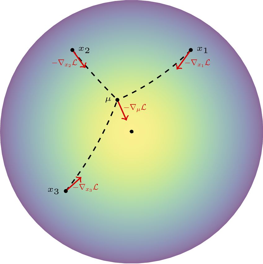
are defined as compositions of Euclidean layers. Figure 2. Depicted above is the Fréchet mean, µ, of three points,
x1 , x2 , x3 in the Poincaré ball model of hyperbolic space, D2−1 , as
well as the negative gradients (shown in red) with respect to the
4. A Differentiable Fréchet Mean Operation loss function L = kµk2 .
for General Riemannian Manifolds
In this section, we provide a few theorems that summarize
our method of differentiating through the Fréchet mean. 4.2. Differentiating Through the Fréchet Mean
4.1. Background on the Fréchet Mean All known methods for computing the Fréchet mean rely
on some sort of iterative solver (Gu et al., 2019). While
Fréchet mean and variance: On a Riemannian manifold backpropagating through such a solver is possible, it is com-
(M, ρ), the Fréchet mean µf r ∈ M and Fréchet variance putationally inefficient and suffers from numerical instabil-
σf2 r ∈ R of a set of points B = {x(1) , · · · , x(t) } with each ities akin to those found in RNNs (Pascanu et al., 2013).
x(l) ∈ M are defined as the solution and optimal values of To circumvent these issues, recent works compute gradi-
the following optimization problem (Bacák, 2014): ents at the solved value instead of differentiating directly,
allowing for full neural network integration (Chen et al.,
1X
t 2018; Pogančić et al., 2020). However, to the best of our
µf r = arg min d(x(l) , µ)2 (3) knowledge, no paper has investigated backpropagation on a
µ∈M t
l=1 manifold-based convex optimization solver. Hence, in this
t section, we construct the gradient, relying on the fact that
1X
σf2 r = min d(x(l) , µ)2 (4) the Fréchet mean is an argmin operation.
µ∈M t
l=1
4.2.1. D IFFERENTIATING THROUGH THE ARGMIN
In Appendix A, we provide proofs to illustrate that this O PERATION
definition is a natural generalization of Euclidean mean and
variance. Motivated by previous works on differentiating argmin prob-
lems (Gould et al., 2016), we propose a generalization which
The Fréchet mean can be further generalized with an ar- allows us to differentiate the argmin operation on the mani-
bitrary re-weighting. In particular, for positive weights fold. The full theory is presented in Appendix D.
{wl }l∈[t] , we can define the weighted Fréchet mean as:
4.2.2. C ONSTRUCTION OF THE F R ÉCHET MEAN
t
X
(l) 2 DERIVATIVE
µf r = arg min wl · d(x , µ) (5)
µ∈M
l=1 Since the Fréchet mean is an argmin operation, we can apply
the theorems in Appendix D to obtain gradients with respect
This generalizes the weighted Euclidean mean to Rieman- to the input points. This operation (as well the resulting
nian manifolds. gradients) are visualized in Figure 2.Differentiating through the Fréchet Mean
For the following theorems, we denote ∇ e as the total deriva- to properly integrate it in the hyperbolic setting we need to
tive (or Jacobian) for notational convenience. address two major difficulties:
Theorem 4.1. Let M be an n-dimensional Riemannian
manifold, and let {x} = (x(1) , . . . , x(t) ) ∈ (M)t be a set of
1. The lack of a fast forward computation.
data points with weights w1 , . . . , wt ∈ R+ . Let f : (M)t ×
t
wl · d(x(l) , y)2 and
P
M → M be given by f ({x} , y) =
l=1 2. The lack of an explicit derivation of a backpropagation
x = µf r ({x}) = arg miny∈M f ({x}, y) be the Fréchet formula.
mean. Then with respect to local coordinates we have
e x(i) µf r ({x}) = −fY Y ({x} , x)−1 fX (i) Y ({x} , x) (6)
∇ Resolving these difficulties will allow us to define a Fréchet
mean neural network layer for geometric, and specifically
where the functions fX (i) Y ({x} , y) = ∇
e x(i) ∇y f ({x} , y) hyperbolic, machine learning tasks.
2
and fY Y ({x} , y) = ∇yy f ({x} , x) are defined in terms of
local coordinates. 5.1. Forward Computation of the Hyperbolic Fréchet
Mean
Proof. This is a special case of Theorem D.1 in the ap- Previous forward computations fall into one of two cat-
pendix. This is because the Fréchet objective function f is egories: (1) fast, inaccurate computations which aim to
a twice differentiable real-valued function for specific x(i) approximate the true mean with a pseudo-Fréchet mean,
and y (under our geodesic formulation); thus we obtain the or (2) slow, exact computations. In this section we focus
desired formulation. The full explanation can be found in on outperforming methods in the latter category, since we
Remark D. strive to compute the exact Fréchet mean (pseudo-means
warp geometry).
While the above theorem gives a nice theoretical framework
with minimal assumptions, it is in practice too unwieldy to 5.1.1. F ORMER ATTEMPTS AT C OMPUTING THE
apply. In particular, the requirement of local coordinates F R ÉCHET M EAN
renders most computations difficult. We now present a ver-
sion of the above theorem which assumes that the manifold The two existing algorithms for Fréchet mean computation
is embedded in Euclidean space4 . are (1) Riemannian gradient-based optimization (Gu et al.,
2019) and (2) iterative averaging (Karcher, 1977). However,
Theorem 4.2. Assume the conditions and values in Theo- in practice both algorithms are slow to converge even for
rem 4.1. Furthermore, assume M is embedded (as a Rie- simple synthetic examples of points in hyperbolic space. To
mannian manifold) in Rm with m ≥ dim M, then we can overcome this difficulty, which can cripple neural networks,
write we propose the following algorithm that is much faster in
e x(i) µf r ({x}) = −f p ({x} , x)−1 f p (i) ({x} , x) (7) practice.
∇ YY X Y
Algorithm 1 Poincaré model Fréchet mean algorithm
where fYp Y ({x} , y) = ∇ e y (projT M ◦∇y f )({x} , y),
p
x
Inputs: x(1) , · · · , x(t) ∈ DnK ⊆ Rn+1 and weights
fX (i) Y ({x} , y) = ∇
e x(i) (projT M ◦∇y f )({x} , y), and
x
w 1 , . . . , w t ∈ R+ .
projTx M : Rm → Tx M ∼ = Rn is the linear subspace
Algorithm:
projection operator.
y0 = x(1)
Define g(y) = 2 arccosh(1+2y)
√ 2
Proof. Similar to the relationship between Theorem 4.1 and y +y
Theorem D.1, this is a special case of Theorem D.3 in the for k = 0, 1, · · · , T :
appendix. for l = 1, 2, · · ·, t:
kx(l) −yk k2 1
αl = wl g (1+Kkx(l) k2 )(1+Kkyk k2 ) 1+Kkx(l) k2
5. Hyperbolic Fréchet Mean t t t
αl x(l) , c = αl kx(l) k2
P P P
a= αl , b =
Although we have provided a formulation for differentiating l=1 l=1 l=1
√
through the Fréchet mean on general Riemannian manifolds, (a−cK)− (a−cK)2 +4K·kbk2
yk+1 = 2|K|·kbk2 b
4
We also present a more general way to take the derivative that return yT
drops this restriction via an exponential map-based parameteriza-
tion in Appendix D.Differentiating through the Fréchet Mean
5.1.2. A LGORITHM FOR F R ÉCHET M EAN 5.1.3. E MPIRICAL C OMPARISON TO P REVIOUS
C OMPUTATION VIA F IRST- ORDER B OUND F R ÉCHET M EAN C OMPUTATION A LGORITHMS
The core idea of our algorithm relies on the fact that the To demonstrate the efficacy of our algorithm, we com-
square of distance metric is a concave function for both the pare it to previous approaches on randomly generated data.
Poincaré ball and hyperboloid model. Intuitively, we select Namely, we compare against a naı̈ve Riemannian Gradi-
an initial “guess” and use a first-order bound to minimize ent Descent (RGD) approach (Udrişte, 1994) and against
the Fréchet mean objective. The concrete algorithm for the the Karcher Flow algorithm (Karcher, 1977). We test
Poincaré ball model is given as Algorithm 1 above. Note our Fréchet mean algorithm against these methods on syn-
that the algorithm is entirely hyperparameter-free and does thetic datasets of ten on-manifold randomly generated 16-
not require setting a step-size. Additionally we introduce dimensional points. We run all algorithms until they are
three different initializations: within = 10−12 of the true Fréchet mean in norm, and
report the number of iterations this takes in Table 3 for
1. Setting y0 = x(1) . both hyperboloid (H) and Poincaré (P) models of hyper-
bolic space. Note that we significantly outperform the other
2. Setting y0 = x(arg maxi wi ) . algorithms. We also observe that by allowing 200x more
computation, a grid search on the learning hyperparame-
3. Setting y0 to be the output of the first step of the
ter6 in RGD obtains nearly comparable or better results
Karcher flow algorithm (Karcher, 1977).
(last row of Table 3 for both models). However, we stress
that this requires much more computation, and note that
We tried these initializations for our test tasks (in which
our algorithm produces nearly the same result while being
weights were equal, tasks described in Section 6), and
hyperparameter-free.
found little difference between them in terms of perfor-
mance. Even for toy tasks with varying weights, these three
methods produced nearly the same results. However, we
give them here for completeness. Table 3. Empirical computation of the Fréchet mean; the average
number of iterations, as well as runtime, required to become ac-
Moreover, we can prove that the algorithm is guaranteed to
curate within = 10−12 of the true Fréchet mean are reported.
converge. 10 trials are conducted, and standard deviation is reported. The
Theorem 5.1. Let x(1) , · · · , x(t) ∈ DnK be t points5 in the primary baselines are the RGD (Udrişte, 1994) and Karcher Flow
Poincaré ball, w1 , . . . , wt ∈ R+ be their weights, and let (Karcher, 1977) algorithms. (H) refers to hyperboloid and (P)
their weighted Fréchet mean be the solution to the following refers to Poincaré.
optimization problem. .
Iterations Time (ms)7
µf r = arg min f (y) (8) RGD (lr = 0.01) 801.0±21.0 932.9±130.0
y∈Dn
K Karcher Flow 62.5±6.0 50.9±8.9
H
Ours 13.7±0.9 6.1±1.9
t
X
where f (y) = wl · dDnK (x(l) , y)2 RGD + Grid Search on lr 27.7±0.8 5333.5±770.7
l=1 RGD (lr = 0.01) 773.8±22.1 1157.3±74.8
t
! Karcher Flow 57.5±9.1 59.8±10.4
wl 2Kkx(l) − yk2
P
X
= arccosh2 1− Ours 13.4±0.5 9.1±1.3
|K| (1 + Kkx(l) k2 )(1 + Kkyk2 )
l=1 RGD + Grid Search on lr 10.5±0.5 6050.6±235.2
(9)
Then Algorithm 1 gives a sequence of points {yk } such that
their limit lim yk = µf r converges to the Fréchet mean
k→∞
solution. We also find that this convergence improvement translates
to real world applications. Specifically, we find that for the
graph link prediction experimental setting in Section 6.1.3,
Proof. See Theorem E.2 in the appendix.
our forward pass takes anywhere from ≈ 15 − 25 iterations,
significantly outperforming the 1000+ needed with RGD
The algorithm and proof of convergence for the hyperboloid
and ≈ 120 needed with Karcher Flow.
model are given in Appendix E.1 and are omitted here for
6
brevity. The grid search starts from lr = 0.2 and goes to lr = 0.4 in
increments of 0.01 for the Poincaré ball model, and from lr = 0.2
5 to 0.28 for the hyperboloid model (same increment).
Here we present the version for K = −1 for cleaner presen-
7
tation. The generalization to arbitrary K < 0 is easy to compute, Experiments were run with an Intel Skylake Core i7-6700HQ
but clutters presentation. 2.6 GHz Quad core CPU.Differentiating through the Fréchet Mean
5.2. Backward Computation of the Hyperbolic Fréchet Fréchet mean layer. This was the original intent10 but was
Mean not feasible without our formulation. In the second setting,
we introduce Hyperbolic Batch Normalization (HBN) as
For the backward computation, we re-apply the general Rie-
an extension of the regular Euclidean Batch Normalization
mannian theory for differentiating through the Fréchet mean
(EBN). When combined with hyperbolic neural networks
in Section 4 to hyperbolic space. Since most autodiffer-
(Ganea et al., 2018), HBN exhibits benefits similar to those
entiation packages do not support manifold-aware higher
of EBN with Euclidean networks.
order differentiation, we derive the gradients explicitly. We
begin with the Poincaré ball model by setting M = DnK
6.1. Hyperbolic Graph Convolutional Neural Networks
and applying Theorem 4.2.
(HGCNs)
Theorem 5.2. Let x(1) , · · · , x(t) ∈ DnK ⊆ Rn be t points
in the Poincaré ball and w1 , . . . , wt ∈ R+ be the weights. 6.1.1. O RIGINAL F RAMEWORK
Let their weighted Fréchet mean µf r be solution to the Introduced in Chami et al. (2019), Hyperbolic Graph Con-
following optimization problem volutional Networks (GCNs) provide generalizations of Eu-
clidean GCNs to hyperbolic space. The proposed network
µf r (x(1) , · · · , x(t) ) = arg min f ({x}, y) (10) architecture is based on three different layer types: feature
y∈Dn
K
transformation, activation, and attention-based aggregation.
t
X Feature transformation: The hyperbolic feature transfor-
where f ({x}, y) = wl · dDnK (x(l) , y)2 = mation consists of a gyrovector matrix multiplication fol-
l=1 lowed by a gyrovector addition.
t
!
X wl 2K||x(l) − y||22
arccosh2 1− hli = (W l ⊗Kl−1 xl−1
i )⊕
Kl−1 l
b (13)
|K|
l=1
(1 + K||x(l) ||22 )(1 + K||y||22 )
(11)
Attention-based aggregation: Neighborhood aggregation
Then the derivative of µf r with respect to x(i) is given by
combines local data at a node. It does so by projecting the
neighbors using the logarithmic map at the node, averaging
e x(i) µf r ({x}) = −fY Y f ({x} , x)−1 fX (i) Y ({x} , x)
∇ in the tangent space, and projecting back with the exponen-
(12) tial map at the node. Note that the weights wij are positive
where x = µf r ({x}) and fY Y , fX (i) Y are defined in Theo- and can be trained or defined by the graph adjacency matrix.
rem 4.2 8 .
X
The full concrete derivation of the above terms for the geom- AGGK (xi ) = expK xi
wij logK
xi xj
(14)
etry induced by this manifold choice is given in Appendix j∈N (i)
Theorem F.3.
Activation: The activation layer applies a hyperbolic acti-
Proof. This is a concrete application of Theorem 4.2. In vation function.
particular since our manifold is embedded in Rn (DnK ⊆ Kl−1 ,Kl
xli = σ ⊗ (yil ) (15)
Rn ). Note that this is the total derivative in the ambient
Euclidean space9 . For the full proof see Theorem F.3 in the
6.1.2. P ROPOSED C HANGES
Appendix.
The usage of tangent space aggregation in the HGCN frame-
The derivation for the hyperboloid model is given in Ap- work stemmed from the lack of a differentiable Fréchet
pendix F.2. mean operation. As a natural extension, we substitute our
Fréchet mean in place of the aggregation layer.
6. Case Studies 6.1.3. E XPERIMENTAL R ESULTS
To demonstrate the efficacy of our developed theory, we We use precisely the same architecture as in Chami et al.
investigate the following test settings. In the first setting, we (2019), except we substitute all hyperbolic aggregation lay-
directly modify the hyperbolic aggregation strategy in Hy- ers with our differentiable Fréchet mean layer. Furthermore,
perbolic GCNs (Chami et al., 2019) to use our differentiable
10
We quote directly from the paper Chami et al. (2019): “An
8
The projection operation is trivial since dim Rn = dim Dn
K. analog of mean aggregation in hyperbolic space is the Fréchet
9
To transform Euclidean gradients into Riemannian ones, sim- mean, which, however, has no closed form solution. Instead, we
ply multiply by inverse of the matrix of the metric. propose to...”Differentiating through the Fréchet Mean
we test with precisely the same hyperparameters (learning yields better final results (Santurkar et al., 2018). Generaliz-
rate, test/val split, and the like) as Chami et al. (2019) for a ing this for Riemannian manifolds is a natural extension, and
fair comparison. Our new aggregation allows us to achieve such a computation would involve a differentiable Fréchet
new state-of-the-art results on the Disease and Disease-M mean.
graph datasets (Chami et al., 2019). These datasets induce
ideal test tasks for hyperbolic learning since they have very 6.2.1. T HEORETICAL F ORMULATION AND A LGORITHM
low Gromov δ-hyperbolicity (Adcock et al., 2013), which
In this section we formulate Riemannian Batch Normal-
indicates the structure is highly tree-like. Our results and
ization as a natural extension of standard Euclidean Batch
comparison to the baseline are given in Table 4. We run
Normalization. This concept is, to the best of our knowl-
experiments for 5 trials and report the mean and standard
edge, only touched upon by Brooks et al. (2019) in the
deviation. Due to practical considerations, we only test with
specific instance of the manifold of positive semidefinite
the Poincaré model11 . For reference, the strongest base-
matrices. However, we argue in Appendix G that, unlike our
line results with the hyperboloid model are reported from
method, their formulation is incomplete and lacks sufficient
Chami et al. (2019) (note that we outperform these results as
generality to be considered a true extension.
well). On the rather non-hyperbolic CoRA (Sen et al., 2008)
dataset, our performance is comparable to that of the best
baseline. Note that this is similar to the performance exhib- Algorithm 2 Riemannian Batch Normalization
ited by the vanilla HGCN. Hence we conjecture that when (t) (t)
Training Input: Batches of data points {x1 , · · · , xm } ⊆
the underlying dataset is not hyperbolic in nature, we do M for t ∈ [1, . . . , T ], testing momentum η ∈ [0, 1]
not observe improvements over the best Euclidean baseline Learned Parameters: Target mean µ0 ∈ M, target vari-
methods. ance (σ 0 )2 ∈ R
Training Algorithm:
(1) (1)
Table 4. ROC AUC results for Link Prediction (LP) on various µtest ← FrechetMean({x1 , . . . , xm })
graph datasets, averaged over 5 trials (with standard deviations). σtest ← 0
Graph hyperbolicity values are also reported (lower δ is more for t = 1, . . . , T :
(t) (t)
hyperbolic). Results are given for models learning in Euclidean µ = FrechetMean({x1 , . . . , xm })
(E), Hyperboloid (H), and Poincaré (P) spaces. Note that the best m
1 (t)
σ2 = m d(xi , µ)2
P
Euclidean method is GAT (Veličković et al., 2018) and is shown
i=1
below for fair comparison on CoRA. We highlight the best result µtest = FrechetMean({µtest , µ}, {η, 1 − η})
only if our result gives a p-value < 0.01 after running a paired-
significance t-test.
σtest = (t−1)σttest +σ
for i = 1, · · · , m:
Disease Disease-M CoRA 0 (t)
x̃i (t) ← expµ0 σσ P Tµ→µ0 (logµ xi )
δ=0 δ=0 δ = 11
return normalized batch x˜1 (t) , · · · , x˜m (t)
MLP 72.6±0.6 55.3±0.5 83.1±0.5
E
GAT 69.8±0.3 69.5±0.4 93.7±0.1 Testing Input: Test data points {x1 , · · · , xs } ⊆ M, final
HNN 75.1±0.3 60.9±0.4 89.0±0.1 running mean µtest and running variance σtest
H
HGCN 90.8±0.3 78.1±0.4 92.9±0.1 Testing Algorithm:
µ = FrechetMean({x1 , · · · , xs })
HGCN 76.4±8.9 81.4±3.4 93.4±0.4 m
P
1
σ2 = m d(xi , µ)2
P
Ours 93.7±0.4 91.0±0.6 92.9±0.4
i=1
for i = 1, · · · , s:
x̃i ← expµtest σtest
σ P Tµ→µtest (logµ xi )
6.2. Hyperbolic Batch Normalization
return normalized batch x˜1 , · · · , x˜s
Euclidean batch normalization (Ioffe & Szegedy, 2015) is
one of the most widely used neural network operations that
Our full algorithm
√ is given in Algorithm 2. Note that in
has, in many cases, obviated the need for explicit regulariza-
practice we use σ 2 + in place of σ as in the original
tion such as dropout (Srivastava et al., 2014). In particular,
formulation to avoid division by zero.
analysis demonstrates that batch normalization induces a
smoother loss surface which facilitates convergence and
6.2.2. E XPERIMENTAL R ESULTS
11
The code for HGCN included only the Poincaré model imple-
mentation at the time this paper was submitted. Hence we use the We apply Riemannian Batch Normalization (specifically
Poincaré model for our experiments, although our contributions for hyperbolic space) to the encoding Hyperbolic Neural
include derivations for both hyperboloid and Poincaré models. Network (HNN) (Ganea et al., 2018) in the framework ofDifferentiating through the Fréchet Mean
Figure 3. The graphs above correspond to a comparison of the HNN baseline, which uses a two-layer hyperbolic neural network encoder,
and the baseline augmented with hyperbolic batch normalization after each layer. The columns correspond to the CoRA (Sen et al., 2008),
Disease (Chami et al., 2019), and Disease-M (Chami et al., 2019) datasets, respectively. The top row shows the comparison in terms of
validation loss, and the bottom row shows the comparison in terms of validation ROC AUC. The figures show that we converge faster and
attain better performance in terms of both loss and ROC. Note that although CoRA is not hyperbolic (as previously mentioned), we find it
encouraging that introducing hyperbolic batch normalization produces an improvement regardless of dataset hyperbolicity.
Chami et al. (2019). We run on the CoRA (Sen et al., 2008), tended batch normalization (a standard Euclidean operation)
Disease (Chami et al., 2019), and Disease-M (Chami et al., to the realm of hyperbolic space. On a graph link prediction
2019) datasets and present the validation loss and ROC AUC test task, we showed that hyperbolic batch normalization
diagrams in Figure 3. gives benefits similar to those experienced in the Euclidean
setting.
In terms of both loss and ROC, our method results in both
faster convergence and a better final result. These improve- We hope our work paves the way for future developments in
ments are expected as they appear when applying standard geometric representation learning. Potential future work can
batch normalization to Euclidean neural networks. So, our focus on speeding up our computation of the Fréchet mean
manifold generalization does seem to replicate the useful gradient, finding applications of our theory on manifolds
properties of standard batch normalization. Additionally, beyond hyperbolic space, and applying the Fréchet mean to
it is encouraging to see that, regardless of the hyperbolic generalize more standard neural network operations.
nature of the underlying dataset, hyperbolic batch normal-
ization produces an improvement when paired with a hyper- 8. Acknowledgements
bolic neural network.
We would like to acknowledge Horace He for his helpful
7. Conclusion and Future Work comments regarding implementation. In addition, we would
like to thank Facebook AI for funding equipment that made
We have presented a fully differentiable Fréchet mean opera- this work possible.
tion for use in any differentiable programming setting. Con-
cretely, we introduced differentiation theory for the general References
Riemannian case, and for the demonstrably useful case of
hyperbolic space, we provided a fast forward pass algorithm Adcock, A. B., Sullivan, B. D., and Mahoney, M. W. Tree-
and explicit derivative computations. We demonstrated that like structure in large social and information networks.
using the Fréchet mean in place of tangent space aggrega- 2013 IEEE 13th International Conference on Data Min-
tion yields state-of-the-art performance on link prediction ing, pp. 1–10, 2013.
tasks in graphs with tree-like structure. Additionally, we ex-
Agrawal, A., Amos, B., Barratt, S., Boyd, S., Diamond,Differentiating through the Fréchet Mean
S., and Kolter, J. Z. Differentiable convex optimization Ioffe, S. and Szegedy, C. Batch normalization: Accelerating
layers. In Advances in Neural Information Processing deep network training by reducing internal covariate shift.
Systems, pp. 9558–9570, 2019. In International Conference on Machine Learning, pp.
448–456, 2015.
Amos, B. and Kolter, J. Z. Optnet: Differentiable optimiza-
tion as a layer in neural networks. In Proceedings of Karcher, H. Riemannian center of mass and mollifier
the 34th International Conference on Machine Learning- smoothing. Communications on Pure and Applied Math-
Volume 70, pp. 136–145, 2017. ematics, 30(5):509–541, 1977.
Bacák, M. Computing medians and means in hadamard Kleinberg, R. D. Geographic routing using hyperbolic space.
spaces. SIAM Journal on Optimization, 24(3):1542–1566, IEEE INFOCOM 2007 - 26th IEEE International Con-
2014. ference on Computer Communications, pp. 1902–1909,
Brooks, D., Schwander, O., Barbaresco, F., Schneider, J.- 2007.
Y., and Cord, M. Riemannian batch normalization for
Law, M., Liao, R., Snell, J., and Zemel, R. Lorentzian dis-
spd neural networks. In Advances in Neural Information
tance learning for hyperbolic representations. In Interna-
Processing Systems, pp. 15463–15474, 2019.
tional Conference on Machine Learning, pp. 3672–3681,
Casado, M. L. Trivializations for gradient-based optimiza- 2019.
tion on manifolds. In Advances in Neural Information
Processing Systems, pp. 9154–9164, 2019. Lee, J. Riemannian Manifolds: An Introduction to Curva-
ture. Graduate Texts in Mathematics. Springer New York,
Chami, I., Ying, Z., Ré, C., and Leskovec, J. Hyperbolic 1997.
graph convolutional neural networks. In Advances in
Neural Information Processing Systems, pp. 4869–4880, Lee, J. M. Introduction to smooth manifolds. Graduate
2019. Texts in Mathematics, 218, 2003.
Charlier, B. Necessary and sufficient condition for the exis- Liu, Q., Nickel, M., and Kiela, D. Hyperbolic graph neural
tence of a fréchet mean on the circle. ESAIM: Probability networks. In Advances in Neural Information Processing
and Statistics, 17:635–649, 2013. Systems, pp. 8228–8239, 2019.
Chen, T. Q., Rubanova, Y., Bettencourt, J., and Duvenaud, Nickel, M. and Kiela, D. Poincaré embeddings for learn-
D. K. Neural ordinary differential equations. In Ad- ing hierarchical representations. In Advances in Neural
vances in Neural Information Processing Systems, pp. Information Processing Systems, pp. 6338–6347, 2017.
6571–6583, 2018.
Nickel, M. and Kiela, D. Learning continuous hierarchies
Fréchet, M. Les éléments aléatoires de nature quelconque in the Lorentz model of hyperbolic geometry. In Proceed-
dans un espace distancié. In Annales de l’institut Henri ings of the 35th International Conference on Machine
Poincaré, volume 10, pp. 215–310, 1948. Learning, pp. 3779–3788, 2018.
Ganea, O., Bécigneul, G., and Hofmann, T. Hyperbolic
Pascanu, R., Mikolov, T., and Bengio, Y. On the difficulty
neural networks. In Advances in Neural Information
of training recurrent neural networks. In International
Processing Systems, pp. 5345–5355, 2018.
Conference on Machine Learning, pp. 1310–1318, 2013.
Gould, S., Fernando, B., Cherian, A., Anderson, P., Cruz,
R. S., and Guo, E. On differentiating parameterized Pogančić, M. V., Paulus, A., Musil, V., Martius, G., and
argmin and argmax problems with application to bi-level Rolinek, M. Differentiation of blackbox combinatorial
optimization. ArXiv, abs/1607.05447, 2016. solvers. In International Conference on Learning Repre-
sentations, 2020.
Gu, A., Sala, F., Gunel, B., and Ré, C. Learning mixed-
curvature representations in product spaces. In Interna- Sala, F., Sa, C. D., Gu, A., and Ré, C. Representation
tional Conference on Learning Representations, 2019. tradeoffs for hyperbolic embeddings. Proceedings of
Machine Learning Research, 80:4460–4469, 2018.
Gulcehre, C., Denil, M., Malinowski, M., Razavi, A., Pas-
canu, R., Hermann, K. M., Battaglia, P., Bapst, V., Ra- Santurkar, S., Tsipras, D., Ilyas, A., and Madry, A. How
poso, D., Santoro, A., and de Freitas, N. Hyperbolic atten- does batch normalization help optimization? In Ad-
tion networks. In International Conference on Learning vances in Neural Information Processing Systems, pp.
Representations, 2019. 2483–2493, 2018.Differentiating through the Fréchet Mean Sarkar, R. Low distortion delaunay embedding of trees in hyperbolic plane. In Proceedings of the 19th International Conference on Graph Drawing, GD’11, pp. 355–366, Berlin, Heidelberg, 2011. Springer-Verlag. Sen, P., Namata, G., Bilgic, M., Getoor, L., Gallagher, B., and Eliassi-Rad, T. Collective classification in network data. AI Magazine, 29:93–106, 2008. Srivastava, N., Hinton, G., Krizhevsky, A., Sutskever, I., and Salakhutdinov, R. Dropout: A simple way to prevent neural networks from overfitting. Journal of Machine Learning Research, 15:1929–1958, 2014. Tifrea, A., Becigneul, G., and Ganea, O.-E. Poincaré glove: Hyperbolic word embeddings. In International Confer- ence on Learning Representations, 2019. Udrişte, C. Convex functions and optimization methods on Riemannian manifolds. Mathematics and Its Ap- plications. Springer, Dordrecht, 1994. doi: 10.1007/ 978-94-015-8390-9. Ungar, A. A. A gyrovector space approach to hyperbolic ge- ometry. Synthesis Lectures on Mathematics and Statistics, 1(1):1–194, 2008. Vaswani, A., Shazeer, N., Parmar, N., Uszkoreit, J., Jones, L., Gomez, A. N., Kaiser, L., and Polosukhin, I. Attention is all you need. ArXiv, abs/1706.03762, 2017. Veličković, P., Cucurull, G., Casanova, A., Romero, A., Liò, P., and Bengio, Y. Graph attention networks. In International Conference on Learning Representations, 2018. Wolter, F.-E. Distance function and cut loci on a complete riemannian manifold. Archiv der Mathematik, 32(1):92– 96, 1979. doi: 10.1007/BF01238473. Yu, T. and De Sa, C. M. Numerically accurate hyperbolic embeddings using tiling-based models. In Advances in Neural Information Processing Systems, pp. 2021–2031, 2019.
You can also read