Demand-Side Scheduling Based on Deep Actor-Critic Learning for Smart Grids - arXiv
←
→
Page content transcription
If your browser does not render page correctly, please read the page content below
SUBMITTED TO ARXIV - 5 MAY 2020                                                                                                         1

                                                       Demand-Side Scheduling Based on Deep
                                                        Actor-Critic Learning for Smart Grids
                                                                                    Joash Lee, Wenbo Wang, and Dusit Niyato

                                           Abstract—We consider the problem of demand-side energy                 noted in [1], residential consumers are usually risk-averse and
                                        management, where each household is equipped with a smart                 shorted-sighted; it would be very difficult for consumers to
                                        meter that is able to schedule home appliances online. The goal           schedule for long-term cost optimisation based solely on a
                                        is to minimise the overall cost under a real-time pricing scheme.
arXiv:2005.01979v1 [cs.LG] 5 May 2020

                                        While previous works have introduced centralised approaches,              dynamic price signal. Secondly, compared with the commer-
                                        we formulate the smart grid environment as a Markov game,                 cial or industry consumers, individual residential consumers
                                        where each household is a decentralised agent, and the grid               often appear to exhibit near-random consumption patterns [3].
                                        operator produces a price signal that adapts to the energy                Real-time sensing and communication of data between each
                                        demand. The main challenge addressed in our approach is partial           home’s energy-consumption manager and the utility operator
                                        observability and perceived non-stationarity of the environment
                                        from the viewpoint of each agent. We propose a multi-agent                thus becomes essential.
                                        extension of a deep actor-critic algorithm that shows success in             Under the framework of automatic price-demand schedul-
                                        learning in this environment. This algorithm learns a centralised         ing, a variety of dynamic-response problem formulations have
                                        critic that coordinates training of all agents. Our approach thus         been proposed in the literature. One major category of the
                                        uses centralised learning but decentralised execution. Simulation         existing schemes focuses on direct load control to optimise
                                        results show that our online deep reinforcement learning method
                                        can reduce both the peak-to-average ratio of total energy con-            a certain objective with (possibly) the constraints on grid
                                        sumed and the cost of electricity for all households based purely         capacity and appliance requirement. Typical objectives in this
                                        on instantaneous observations and a price signal.                         scenario can be to minimise energy consumption/costs [4]–[9],
                                           Index Terms—Reinforcement learning, smart grid, deep learn-            maximise the utility of either middlemen or end-users [10]–
                                        ing, multi-agent systems, task scheduling                                 [14], or minimise the peak load demand of the overall
                                                                                                                  system [2], [3], [9]. With such a setup, DSM is usually
                                                                                                                  assumed to be performed in a slotted manner (e.g., with
                                                                I. I NTRODUCTION                                  a time scale measured in hours [2]) within finite stages.
                                           In the past decade, Demand-Side Management (DSM) with                  The DSM problem can be formulated under a centralised
                                        price-based demand response has been widely considered to                 framework as a scheduling problem [3], or an optimisation
                                        be an efficient method of incentivising users to collectively             problem such as a linear program [9] or a stochastic pro-
                                        achieve better grid welfare [1]. In a typical DSM scenario, an            grams [10]. Alternatively, under a decentralised framework,
                                        independent utility operator plans the preferred demand vol-              the DSM problem can also be developed in the form of non-
                                        ume for a certain metering time duration within the considered            cooperative games with specifically designed game structure
                                        micro (e.g., district) grid. In order to achieve this, the operator       to guarantee desired social welfare indices [2]. Apart from
                                        adopts a time-varying pricing scheme and announces the prices             the programming/planning oriented schemes, another major
                                        to the users on a rolling basis. In general, the price may be             category of design emphasises the uncertainties in the DSM
                                        determined by factors such as the demand for the utility, the             process, e.g., due to the random arrival of appliance tasks
                                        supply of the utility, and the history of their volatility. The           or the unpredictability of the future energy prices. In such
                                        adjusted price is released in advance at some time window to              a scenario, DSM planning based on the premise of known
                                        the consumers. In response to the updated electricity prices, the         system model is typically replaced by DSM strategy-learning
                                        users voluntarily schedule or shift their appliance loads with            schemes, which usually address the uncertainty in the system
                                        the aim of minimising their individual costs, hence making it             by formulating the considered dynamics to be Markov Deci-
                                        possible to reduce the energy waste or load fluctuation of the            sion Processes (MDPs) with partially observability [15]. By
                                        considered microgrid (see the example in [2]).                            assuming infinite plays in a stationary environment, optimal
                                           In the framework of dynamic pricing (a.k.a. real-time pric-            DSM strategies are typically learned in various approaches
                                        ing), dynamic demand response on the user side (e.g., at                  of reinforcement learning without knowing the exact system
                                        residential households) relies on the premise of the availability         models [4], [6].
                                        of smart meters and automatic energy-consumption-manager                     In this paper, we propose a DSM problem formulation with
                                        modules installed in each household. This is mainly due to                dynamic prices in a microgrid of residential district, where
                                        two characteristics of residential utility demand. Firstly, as            a number of household users are powered by a single energy
                                                                                                                  aggregator. By equipping the households with energy manager-
                                          Joash Lee is on a scholarship awarded by the Energy Research Institue   enabled smart meters, we aim at distributedly minimising
                                        @ NTU (ERI@N). Wenbo Wang and Dusit Niyato are with the School
                                        of Computer Science and Engineering, Nanyang Technological University     the cost of energy in the grid, under real-time pricing, over
                                        (NTU), Singapore 639798                                                   the long term with deep reinforcement learning. The main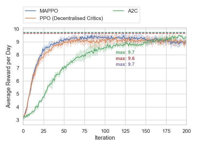
SUBMITTED TO ARXIV - 5 MAY 2020                                                                                                          2

advantage of decentrally controlled energy-managing smart           current state and action are sufficient to describe both the state
meters is that, after the training phase, each household agent      transition model and the reward function.
is able to act independently in the execution phase, without           In this paper, we propose a policy-based algorithm based on
requiring specific information about other households — each        the Proximal Policy Optimisation (PPO) algorithm [22] for a
household agent will not be able to observe the number or           multi-agent framework. We consider the partially observable
nature of devices operated by other households, the amount          Markov game framework [23], which is an extension of the
of energy they individually consume, and when they consume          Markov Decision Process (MDP) for multi-agent systems. A
this energy. Our aforementioned aim addresses at least two          Markov game for N agents can be mathematically described
key challenges. Firstly, the model of the microgrid system and      by a tuple hN , S, {An }n∈N , {On }n∈N , T , {rn }n∈N i, where
its pricing methodology is not available to each household.         N is the set of individual agents and sS describes the overall
Secondly, the limitation in the observation available to each       state of all agents in the environment.
household and the lack of visibility regarding the strategy            At each discrete time step k, each agent n is able to make
of other households creates the local impression of a non-          an observation On of its own state. Based on this observation,
stationary environment. We introduce details of the system          each agent takes an action that is chosen using a stochastic
model in Section III.                                               policy πθn : On 7→ An , where An is the set of all possible
   To overcome the first mentioned key challenge, we propose        actions for agent n. The environment then determines each
a model-free policy-based reinforcement learning method in          agent’s reward as a function of the state and each agent’s
Section IV for each household to learn their optimal DSM            action, such that rn (k) : S × A∞ × · · · × An 7→       > >       > >                 1           M >
                                                                                n , tn , ln , qn ] , where tn = [tn , . . . , tn ] denotes
the MDPs, a common theme was the presence of electricity            the vector of the length of time before the next task for appli-
producers, consumers, and service providers that brokered           ance m can commence, ln = [ln1 , . . . , lnM ]> denotes the vector
trading between them. The reward function in these studies          of task periods, and qn = [qn1 , . . . , qnM ]> denotes the number
were designed to minimise the cost to the service provider          of tasks queued for each appliance. The private observation of
and/or consumer, minimise the discrepancy between the supply        each household consists of its local state augmented with the
and demand of energy or, in the case of [14], maximise the          price of electricity at the previous time step p(k −1), such that
profit achieved by the service provider. A common limitation        on = [x>      > >       >            >
                                                                             n , tn , ln , qn , p(k − 1)] . The overall state is simply
between [7], [12], [13], [18] was the use of tabular Q-learning     the joint operational state of all the users:
limited the algorithm to processing only discretised state and
action spaces.                                                                               s = [s1 , . . . , sN ].                  (1)
   Recently, there have also been studies that have introduced        The task arrival for each appliance corresponds to the
methods utilising deep neural networks to multi-agent rein-         household’s demand to turn it on, and is based on a four-week
forcement learning, albeit to different classes of problems         period of actual household data from the Smart* dataset [24].
[19]–[21]. These newly introduced methods are extensions            We first discretise each day into a set of H time intervals
of the now-canonical deep Q-network (DQN) algorithm for             H = {0, 1, 2, ..., H − 1} of length T , where each interval
the multi-agent environment, and a common technique is to           corresponds to the wall-clock time in the simulated system.
have a central value-function approximator to share infor-          The wall-clock time interval for each time-step in the Markov
mation. However, as explained in section III, a value-based         game is determined with the following relation:
RL algorithm would not suit the problem introduced in this
paper because it requires the Markov assumption that the                                 h(k) =       mod (k, H).                     (2)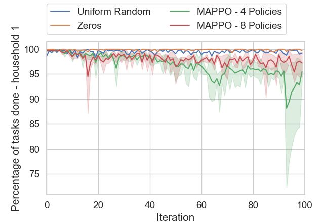
SUBMITTED TO ARXIV - 5 MAY 2020                                                                                                       3

    Next, we count the number of events in each interval               The reward signal then sent to each household is a weighted
where the above-mentioned appliances of interest were turned         sum of a cost objective and a soft constraint.
on. This is used to compute an estimate for the probability
each appliance receives a new task during each time interval,                        rn (k) = −rc,n (k) + wre,n (k)                (6)
                                                  0m
pmn (h(k)). The task arrival for each appliance q n at each time        The first component of the reward function rc,n is the
interval k is thus modelled with a Bernoulli distribution. Each      monetary cost incurred by each household at the end of each
                 m
task arrival q 0 n for a particular appliance m in household n       time step. The negative sign of the term (7) in (6) encourages
is added to a queue qnm .                                            the policy to delay energy consumption until the price is
    The duration of the next task to be executed is denoted          sufficiently low.
by lnm . Its value is updated by randomly sampling from an
exponential distribution whenever a new task is generated (i.e.                          rc,n (k) = p(k) × En (k)                  (7)
    m
q 0 n = 1). The rate parameter λm n for the distribution for each
appliance is assigned to be the reciprocal of the approximate           The second component of the reward is a soft constraint
average duration of tasks in the above-mentioned four-week           re,n tunable by weight w. The soft constraint encourages the
period selected from the Smart* dataset [24]. We choose to           policy to schedule household appliances at a rate that matches
keep the task duration constrained to l ∈ [T, ∞].                    the average rate of task arrival into the queue.
    The use of the described probabilistic models for generation                            re,n (k) = En (k)                      (8)
of task arrivals and task lengths enable us to capture the
variation in household energy demand throughout the course              We adopt a practical assumption that each household can
of an average day while preserving stochasticity in energy           only observe its own internal state along with the published
demand at each household.                                            price at the previous time step, and receive its own cost in-
    We consider that each household’s scheduler is synchronised      curred as the reward signal. For each household n, the system
to operate with the same discrete time steps of length T . At        is thus partially observed, where on (k) = [sn (k)> , p(k−1)]> .
the start of a time step, should there be a task that has newly         We note that the state transition for all households can be
arrived into an empty queue (qnm = 1), the naive strategy            considered to be Markovian because the transition to the next
of inaction would have the task start immediately such that          overall system state is dependent on the current state and the
tm
 n = 0. This corresponds with the conventional day-to-day
                                                                     actions of all household agents: T : S × A1 × · · · × An → S 0 .
scenario where a household appliance turns on immediately            In contrast, we recall from (5) and (6) that the price of energy,
when the user demands so. However, in this paper we consider         and consequently each agent’s reward, is a function of not only
a setting where each household has an intelligent scheduler          the current state and actions, but also of the history of previous
that is capable of acting by delaying each appliance’s starting      states. Our pricing-based energy demand management process
time by a continuous time period am  n ∈ [0, T ]. The joint action
                                                                     is, therefore, a generalisation of the Markov game formulation
of all users is thus:                                                [26].

                      a = [a1 , . . . , aN ]> .               (3)         IV. S EMI -D ISTRIBUTED D EEP R EINFORCEMENT
                                                                                 L EARNING FOR TASK S CHEDULING
   Once an appliance has started executing a task from its
queue, qnm is shortened accordingly. We consider that the               The DSM microgrid problem that we introduce in the
appliance is uninterruptible and operates with a constant power      previous section presents various constraints and difficulties in
consumption Pnm . If an appliance is in operation for any length     solving it: (i) each household can choose its action based only
of time during a given time step, we consider its operational        on its local observation and the last published price, (ii) the
state to be xm                     m                                 reward function is dependent on the states and actions beyond
              n = 1. Otherwise, xn = 0.
                                                                     the last timestep, (iii) the state and observation spaces are
   Let dmn (k) denote the length of time that an appliance m is
                                                                     continuous, (iv) the household agents have no communication
in operation during time step k for household n. The energy
                                                                     channels between them, and (v) a model of the environment is
consumption of a household En (k) during time step k is thus:
                                                                     not available. Constraint (iv) is related to the general problem
                               M
                               X                                     of environmental non-stationarity: concurrent training of all
                   En (k) =          dm     m
                                      n (k)Pn .               (4)    agents would cause the environmental dynamics to constantly
                              m=1                                    change from the perspective of a single agent, thus violating
                                                                     Markov assumptions.
   On the grid side, we consider a dynamic energy price p(k)            Requirements (i) and (ii) and environmental non-stationarity
that is a linear function of the Peak-Average-Ratio [9], [25]        mean that a value-based algorithm such as Q-learning is not
of the energy consumption in the previous κ time steps:              suitable, because these algorithms depend on the Markov
                                                                     assumption that the state transition and reward functions are
                                         N
                        κT     max
                                         P
                                               En (k)                dependent only on the state and action of a single agent at
                             k−κ+1≤k n=1                             the last time step. Furthermore, requirement (v) rules out
               p(k) =                                   .     (5)
                                 N
                                 P                                   model-based algorithms. Thus, in this section, we propose
                                      En (k)                         an extension of the actor-critic algorithm Proximal Policy
                                n=1
SUBMITTED TO ARXIV - 5 MAY 2020                                                                                                            4

Optimisation (PPO) [22] for the multi-agent setting which we
will refer to as Multi-Agent PPO (MAPPO).
   Let π = {π1 , π2 , ..., πN } be the set of policies, parame-
terised by θ = {θ1 , θ2 , ..., θN }, for each of the N agents
in the microgrid. The objective function that we seek to
maximise is P the expected sum of discounted reward J(θ) =
                K
Es∼pπ ,a∼πθ [ k=i γ k−i rk ], where rk is obtained based on (6).
In canonical policy gradient algorithms such as A2C, gradient
ascent is performed to improve the policy:
 ∇θn Jn (θn ) = Es∼pπ ,an ∼πn [∇θn log πn (s, an )Qπnn (s, an )] .
                                                               (9)        Fig. 1: The high-level architecture of the reinforcement learn-
   This policy gradient estimate is known to have high vari-              ing setup with a centralised critic. Each actor and the critic is
ance. It has been shown that this problem is exacerbated in               implemented as a feedforward multi-layer perceptron.
multi-agent settings [19]. For this reason, we propose the im-
plementation of PPO as it limits the size of each policy update
through the use of a surrogate objective function. Additionally,          the N decentralised critic networks to the centralised critic, on
we augment the individually trained actor networks with a                 the assumption that this would result in a similar computation
central critic network V̂ π that approximates the value function          resource requirements.
for each household Vnπ based on the overall system state, thus
receiving information for training of cooperative actions by
individual households. The objective function we propose is                                      V. E XPERIMENTS
the following:                                                              In this section, we present the settings and environmental
                                                                          parameters that we use for experimentation, evaluate our cho-
               h
 L(θn ) = Ek min ρk (θn )Âπn (k), max 1 − ,
                                                        i (10)           sen reinforcement learning method against non-learning agents
                 min(ρk (θn ), 1 + ) Âπn (k) + λH(πn ) ,                and the offline Energy Consumption Scheduler (ECS) method

                                                                          by [9], examine the effect of augmenting local observations in
                       πn (ak |ok )                                       proposed system model, and consider the effects of household
where ρk (θn ) =      πn,old(ak |ok ) ,   and both  and λ are hyperpa-
                                                                          agents learning shared policies.
rameters.  Âπn (k)
                is the estimated advantage value, which is
computed using the critic network:
                                                                          A. System Setup
 Âπn (s, an ) ≈ r(s, an ) + γ V̂ π (s(k + 1))n − V̂ π (s(k))n . (11)
                                                                             We present experiments on a simulated system of identical
   We fit the critic network, parameterised by φ, with the                households, each with 5 household appliances. As mentioned,
following loss function using gradient descent:                           their parameters relating to power consumption Pnm , task
                   XX                           2                       arrival rates pm
                                                                                         n (k) and lengths of operation per use λn are
                                                                                                                                      m
          L(φ) =            V̂ π (s(k))n − yn (k) .   (12)                chosen to be a loose match to data sampled from the Smart*
                         n    k
                                                                          2017 dataset [24], and thus resemble typical household usage
where the target value y(k) = rn (k)+γ V̂ π (s(k+1))n . As the            patterns.
notation suggests, this update is based on the assumption that               The period for each time step T is chosen to be 0.5 hours
the policies of the other agents, and hence their values, remain          to achieve sufficient resolution, while limiting the amount
the same. In theory, the target value must be re-calculated               of computation required for each step of ‘real time’ in the
every time the critic network is updated. However, in practice,           simulation. To reasonably limit the variance of trajectories
we take a few gradient steps at each iteration of the algorithm.          generated, the maximum length of each simulation episode is
   The schematic of the proposed actor-critic frame-                      limited to 240 time steps or 5 days. For each iteration of the
work is illustrated in Figure 1. The centralised critic-                  training algorithm, 5040 time steps of simulation experience
network itself utilises a branched neural network archi-                  is accumulated for each batch. Each experiment is run with a
tecture shown in Figure 2a. To compute the estimated                      number of random seeds; the extent of their effect is shown
state value of a particular household n, Vn , we pro-                     in the range of the lightly shaded regions on either side of the
vide the following input vector to the centralised critic-                lines in the graphs shown.
                                                 > >
network: [ s>    > >        > >          >
            n s1 s2 ... s1 sn−1 sn+1 ...sN ] . The critic network            For this chosen experimental setup, we run two baseline
would
P       thus provide an estimate of the quantity V π (s)n =               performance benchmarks that were non-learning: (i) Firstly, an
   k Eπθ [r(sn , an )|s1 , s2 , . . . , sn−1 , sn+1 , . . . , sN ].       agent that assigned delay actions of zero for all time steps. This
   We compare the MAPPO algorithm to a similar algorithm                  represents the default condition in current households where
that uses a decentralised critic-network instead. The architec-           the user dictates the exact time that all appliances turn on.
ture we utilise for the decentralised critic-network is shown             (ii) A second baseline agent randomly samples delay actions
in Figure 2b. The main consideration for such a design is to              from a uniform distribution with range [0, T ]. We compare
maintain a similar number of learnable parameters across all              these non-learning agents to agents trained using our proposed
SUBMITTED TO ARXIV - 5 MAY 2020 5
(a) (b)
Fig. 2: The architectures of a (a) centralised critic network and a (b) decentralised critic network respectively.
(a) Average reward obtained per day (b) Average monetary cost incurred per day
Fig. 3: Results for a 32-household microgrid system. (a) and (b) show the MAPPO agent’s progress during training, compared
against an agent that samples from a uniform random action distribution, and another that chooses no delays.
Multi-Agent PPO (MAPPO) algorithm as described in Section demand in the night time. The uniform-random-delay agent
IV. dampens these peaks in demand by shifting a number of tasks
The results of the above-mentioned agents are compared in forward into the following time steps (note the lag in energy
Figures 3a and 3b. The y-axis for both graphs shows the aver- consumption compared to the zero-delay agent). In contrast,
age reward gained and average cost incurred by all households the agent trained using reinforcement learning is able to not
for each day within each batch of samples. The x-axis shows just delay the morning peak demand, but spread it out across
the iteration index in the actor-critic training process. (Note the afternoon. The result is a lower PAR, and hence a lower
that each batch consists of 105 days of simulation.) All trained monetary cost per unit energy.
policies demonstrate a sharp improvement in reward achieved Although the morning peak in energy demand is smoothed
from the onset of training. The monetary cost decreases with out by the MAPPO trained households, the same effect is less
increasing reward, showing that the reward function is suitably pronounced for the evening peak. We hypothesise that this
chosen for the objective of minimising cost. was due to the training procedure: the batch of experience
In Figure 4, we plot the average total energy consumed gathered in each iteration of the algorithm began at 00:00
by the entire microgrid system for each half-hour time step. hrs, and terminated at the end of a 24 hour cycle, providing
Note that the x-axis shows the wall-clock in the simulated fewer opportunities for the agents to learn that the evening
environment using the 24 hour format. The blue line shows demand can be delayed to the early hours of the subsequent
the energy-time consumption history if all home appliance day. Moreover, delaying tasks on the last cycle of each batch
were to be run immediately on demand; it reveals the peaks would have led to a lower value of soft-constraint reward re,n ,
in demand in the morning and evening, presumably before but an un-materialised cost improvement (higher rc,n ) for the
and after the home occupants are out to work, and lows in subsequent morning (because of the midnight cut-off).SUBMITTED TO ARXIV - 5 MAY 2020 6
Fig. 4: Average aggregate energy consumed by 32-household Fig. 6: Average reward obtained per day in a 10-household
microgrid for each timestep of the day. microgrid - a comparison with ECS
B. Comparison with ECS
We compare our proposed MAPPO algorithm-based method
to the Energy Consumption Scheduler (ECS) method proposed
by [9], which is also a DSM-based solution. Instead of making
decisions online as with MAPPO, ECS requires the following
information in advance to schedule all energy consumption
for the next day: (i) the total planned energy consumption
for each household appliance for the entire day, and (ii)
the mathematical function used to determine the price of
electricity for a given time period. For a better comparison,
we adapted the experimental setup to match the method used
for ECS in its original paper: we considered a smart grid
system with N = 10 households, split each day into H = 24
equal time intervals, fixed the length of operation of each task
such that lnm = 1/λm n , and used a quadratic price function
as described in (13). We also consider different values of the
multiplier w for the cost constraint in the reward function (6).
Fig. 5: Average aggregate energy consumed by 10-household
pn (k) = b(h) × En (k)2 . (13)
microgrid for each timestep of the day - a comparison between
MAPPO and ECS Input (i) required by the ECS method is thus computed as
follows:
H
X H
X
Enm = (pm m m
n (h) × ln × Pn ) . (14)
The results discussed above are significant for our particular h=1 h=1
application because it shows that while each household is In Figure 5, we plot the average aggregate energy consumed
controlled by different policies, all households are able to by the microgrid for each hour-long time step. Once again,
learn a cooperative strategy that flattens energy demand and the agents trained using reinforcement learning are able to
consequently decrease the average cost for all users. The delay the peaks in demand and spread the energy demand
ability of the agents to learn in a decentralised manner is across subsequent time steps. The MAPPO agents trained with
compatible with a microgrid system where there may be a coefficient of w = 2.2 consume almost the same energy
limited bandwidth to both receive and transmit information over the entire day as the naive agents with zero delay; this
centrally. The individual user, or a small cluster of users, constitutes a shift in energy demand that results in a decrease
could improve their policy using local computing resources, in the cost of energy.
while receiving only the output signal from the centralised In comparison to the MAPPO agents, ECS produces a
critic network. Conversely, if computing resources for neural flatter energy demand profile. Because the ECS algorithm
network training are only available centrally, update gradients receives both the energy consumption requirements and the
can be transmitted to individual actor networks and result in price function before the day commences, it is able to schedule
similar performance. appliances to operate in the early hours of the day to exploitSUBMITTED TO ARXIV - 5 MAY 2020 7
lower prices. However, since the energy consumption require- as part of the observations on perceived by each agent. In an
ments received by ECS are average values, each household 8-household microgrid system, we train MAPPO agents that
experiences a mismatch between its actual energy demand for use observations without the time in one experiment, and train
the day and the schedule produced by ECS. Consequently, we agents with the time but without the previous price in another
compute a reward according to (6), where the value rc,n is experiment. The results are shown in Figure 7.
taken to be the actual energy demand that is fulfilled by the The agents trained without knowledge of the simulation
ECS-generated schedule. The results plotted in Figure 6 show clock time achieve a performance that significantly overlaps
that the MAPPO agents with w = 2.2 achieve an average with the agents trained with the full observation vector. On the
daily reward that is more than 10% higher than that achieved other hand, depriving the agents of knowledge of the price of
by ECS. energy on the previous time step shows both a marked decrease
The results reveal the MAPPO method’s key advantage, in average reward accrued and an increase in the average cost
in that it can be utilised in a fully online scenario without of electricity. The reason is that knowledge of the price at
requiring the price function or the total daily consumption in the previous time step is useful because it indirectly reveals
advance. It is able to rely on instantaneous observations of information about the strategy used by the other household
the local state and the price signal to determine how tasks agents. In making this information observable, the price-
should be scheduled by delaying them. This online approach augmented observation ameliorates the problem of perceived
and reliance on mainly locally observable information is more environmental non-stationarity. In contrast, knowledge of the
consistent with the nature of domestic electricity use. simulation clock time may be less useful because features
Another advantage of MAPPO is that, in addition to shifting within the local state, such as the appliance status xn and
the demand of energy, we are able to implement energy queue lengths qn , already provide time-related queues on how
reduction by tuning the coefficient w. Figure 5 shows that the high the current demand for energy is.
MAPPO agents trained with a smaller coefficient of w = 0.4
exhibit lower energy demand than both the MAPPO agents E. Effect of Policy Sharing
with w = 2.2 and the ECS method.
We consider a scenario where groups of household agents
C. Comparison with Methods using Decentralised Critics may share a common policy. This may be useful when
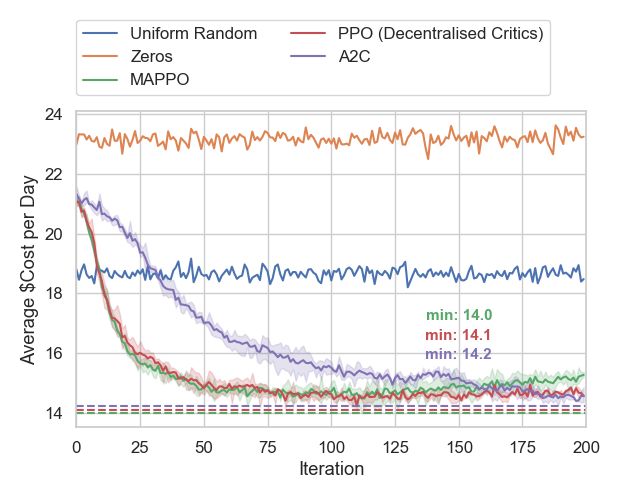
Figures 3a and 3b also compare our proposed MAPPO computing resources are unavailable in individual households,
algorithm to a similar PPO-based algorithm with decentralised but accessible from a more centralised location. Instead of
critics, and the more traditional Advantage Actor-Critic (A2C) having each household agent controlled by a single policy,
[27] algorithm. The results show that all the agents trained we conduct experiments where each policy is shared by two
with deep reinforcement learning perform better than the non- specific household agents. In these setups, each household
learning agents. always follows the same policy network.
Our proposed MAPPO algorithm achieves the most sample- The results are shown in Figure 7. While the reward
efficient learning speed and best performance, while the per- achieved is similar, the systems where agents shared poli-
formance of the decentralised PPO algorithm is close. This cies show a slightly lower resulting cost in energy. This
demonstrates that good performance can also be achieved by is consistent with the findings of [19], which reported that
learning in a completely decentralised manner. This would be sharing ”policy ensembles” resulted in better scores. However,
useful in scenarios where connectivity of the smart meters it should be noted that in the mentioned study, the policies are
outside of the household is limited, but local computing power assigned to randomly chosen agents at each episode.
can be utilised. We investigated further by counting both the number of
The canonical A2C algorithm is also able to reach the tasks generated in the household appliance queues qnm and
same level of performance, although it learns less efficiently the number of tasks done in each time step to compute the
with the same number of samples. Experiments with higher percentage of tasks done by each agent for each episode.
learning rates showed instabilities that manifested in exploding Figure 8 shows the percentage of tasks that were completed
gradients – this was in spite of policy-based algorithms such by household 1 throughout the training process. It reveals that
as A2C being generally known to be more stable than value- the shared policies are able to achieve a lower energy cost
based algorithms. The reason is that, in our proposed microgrid by strategically delaying tasks in the queue (which decreases
environment, the updates to the policies for other households energy consumption). On the other hand, single policies are
under A2C have a large effect on the overall system dynamics, unable to employ the same task-delaying strategy without
possibly worsening the non-stationarity of the environment as overly sacrificing the second component of the reward that
perceived by each household. In contrast, the nature of the encourages task completion.
actor network update in the PPO algorithm limits the change
in the actions taken by the updated policy, thus leading to VI. C ONCLUSION
stable performance increments. In this paper, we proposed and implemented a smart grid en-
vironment, as well as a multi-agent extension of a deep actor-
D. Effect of augmenting local observations critic algorithm for training decentralised household agents to
We perform experiments to determine the necessity of schedule household appliances with the aim of minimising
including the simulation clock time and the previous price the cost of energy under a real-time pricing scheme. OurSUBMITTED TO ARXIV - 5 MAY 2020 8
(a) Average reward obtained per day (b) Average monetary cost incurred per day
Fig. 7: Results for simulation in an 8-household microgrid system. (a) and (b) compare the best results obtained in our
experiments on the effectiveness of augmented observations and policy sharing.
R EFERENCES
[1] J. S. Vardakas, N. Zorba, and C. V. Verikoukis, “A survey on demand
response programs in smart grids: Pricing methods and optimization
algorithms,” IEEE Communications Surveys Tutorials, vol. 17, no. 1,
pp. 152–178, Firstquarter 2015.
[2] R. Deng, Z. Yang, M. Chow, and J. Chen, “A survey on demand
response in smart grids: Mathematical models and approaches,” IEEE
Transactions on Industrial Informatics, vol. 11, no. 3, pp. 570–582, Jun.
2015.
[3] S. Barker, A. Mishra, D. Irwin, P. Shenoy, and J. Albrecht, “Smartcap:
Flattening peak electricity demand in smart homes,” in 2012 IEEE
International Conference on Pervasive Computing and Communications,
2012, Conference Proceedings, pp. 67–75.
[4] F. Ruelens, B. J. Claessens, S. Vandael, B. D. Schutter, R. Babuka,
and R. Belmans, “Residential demand response of thermostatically
controlled loads using batch reinforcement learning,” IEEE Transactions
on Smart Grid, vol. 8, no. 5, pp. 2149–2159, Sep. 2017.
Fig. 8: Percentage of incoming tasks to the queue that were [5] Z. Chen, L. Wu, and Y. Fu, “Real-time price-based demand response
management for residential appliances via stochastic optimization and
completed - household 1. robust optimization,” IEEE Transactions on Smart Grid, vol. 3, no. 4,
pp. 1822–1831, Dec 2012.
[6] Z. Wen, D. O’Neill, and H. Maei, “Optimal demand response using
device-based reinforcement learning,” IEEE Transactions on Smart Grid,
vol. 6, no. 5, pp. 2312–2324, Sep. 2015.
approach allows for an online approach to household appliance [7] B. Kim, Y. Zhang, M. v. d. Schaar, and J. Lee, “Dynamic pricing
scheduling, requiring only the local observation and a price and energy consumption scheduling with reinforcement learning,” IEEE
Transactions on Smart Grid, vol. 7, no. 5, pp. 2187–2198, 2016.
signal from the previous time step to act. A joint critic is [8] E. Mocanu, D. C. Mocanu, P. H. Nguyen, A. Liotta, M. E. Webber,
learned to coordinate training centrally. M. Gibescu, and J. G. Slootweg, “On-line building energy optimization
using deep reinforcement learning,” IEEE Transactions on Smart Grid,
Our results show that our proposed algorithm is able to train vol. 10, no. 4, pp. 3698–3708, 2019.
agents that achieve a lower cost and flatter energy-time profile [9] A. Mohsenian-Rad, V. W. S. Wong, J. Jatskevich, R. Schober, and
A. Leon-Garcia, “Autonomous demand-side management based on
than non-learning agents. Our algorithm also achieves quicker game-theoretic energy consumption scheduling for the future smart
learning than independent agents trained using the canoni- grid,” IEEE Transactions on Smart Grid, vol. 1, no. 3, pp. 320–331,
cal Advantage Actor-Critic (A2C) algorithm. The successful Dec. 2010.
[10] X. Cao, J. Zhang, and H. V. Poor, “Joint energy procurement and demand
results show that the choice of the observed variables and response towards optimal deployment of renewables,” IEEE Journal of
reward function design in our proposed environment contained Selected Topics in Signal Processing, vol. 12, no. 4, pp. 657–672, Aug
sufficient information for learning. 2018.
[11] S. Wang, S. Bi, and Y. J. Angela Zhang, “Reinforcement learning for
Future work can involve extension of the smart grid envi- real-time pricing and scheduling control in ev charging stations,” IEEE
ronment to include more features and real-world complexities; Transactions on Industrial Informatics, pp. 1–1, 2019.
[12] P. P. Reddy and M. M. Veloso, “Strategy learning for autonomous
we identify two such possibilities. Firstly, the architecture of agents in smart grid markets,” in Proceedings of the Twenty-
the microgrid can be expanded to include more energy sources, Second International Joint Conference on Artificial Intelligence, 2011,
which may be operated by producers or households. Secondly, Conference Proceedings. [Online]. Available: https://www.aaai.org/ocs/
index.php/IJCAI/IJCAI11/paper/view/3346/3458
we may expand the overall grid to include more agents and [13] R. Lu, S. H. Hong, and X. Zhang, “A dynamic pricing demand
more types of agents, such as energy producers and brokers. response algorithm for smart grid: Reinforcement learning approach,”SUBMITTED TO ARXIV - 5 MAY 2020 9
Applied Energy, vol. 220, pp. 220–230, 2018. [Online]. Available:
https://www.sciencedirect.com/science/article/pii/S0306261918304112
[14] Y. Yang, J. Hao, M. Sun, Z. Wang, C. Fan, and G. Strbac, “Recurrent
deep multiagent q-learning for autonomous brokers in smart grid,” in
International Joint Conferences on Artificial Intelligence Organization.
International Joint Conferences on Artificial Intelligence Organization,
2018, Conference Proceedings, pp. 569–575. [Online]. Available:
https://doi.org/10.24963/ijcai.2018/79https://goo.gl/HHBYdg
[15] T. M. Hansen, E. K. P. Chong, S. Suryanarayanan, A. A. Maciejewski,
and H. J. Siegel, “A partially observable markov decision process
approach to residential home energy management,” IEEE Transactions
on Smart Grid, vol. 9, no. 2, pp. 1271–1281, March 2018.
[16] H. Zhao, J. Zhao, J. Qiu, G. Liang, and Z. Y. Dong, “Cooperative wind
farm control with deep reinforcement learning and knowledge assisted
learning,” IEEE Transactions on Industrial Informatics, pp. 1–1, 2020.
[17] J. Duan, Z. Yi, D. Shi, C. Lin, X. Lu, and Z. Wang, “Reinforcement-
learning-based optimal control of hybrid energy storage systems in
hybrid acdc microgrids,” IEEE Transactions on Industrial Informatics,
vol. 15, no. 9, pp. 5355–5364, 2019.
[18] E. C. Kara, M. Berges, B. Krogh, and S. Kar, “Using smart devices for
system-level management and control in the smart grid: A reinforcement
learning framework,” in 2012 IEEE Third International Conference
on Smart Grid Communications (SmartGridComm), 2012, Conference
Proceedings, pp. 85–90.
[19] R. Lowe, Y. I. Wu, A. Tamar, J. Harb, O. Pieter Abbeel,
and I. Mordatch, “Multi-agent actor-critic for mixed
cooperative-competitive environments,” in Advances in Neural
Information Processing Systems, 2017, Conference Proceedings,
pp. 6379–6390. [Online]. Available: http://papers.nips.cc/paper/
7217-multi-agent-actor-critic-for-mixed-cooperative-competitive-environments.
pdf
[20] J. Foerster, I. A. Assael, N. de Freitas, and
S. Whiteson, “Learning to communicate with deep multi-
agent reinforcement learning,” in Advances in Neural
Information Processing Systems, 2016, Conference Proceedings,
pp. 2137–2145. [Online]. Available: http://papers.nips.cc/paper/
6042-learning-to-communicate-with-deep-multi-agent-reinforcement-learning.
pdf
[21] T. Rashid, M. Samvelyan, C. Schroeder, G. Farquhar, J. Foerster,
and S. Whiteson, “Qmix: Monotonic value function factorisation
for deep multi-agent reinforcement learning,” in Proceedings of the
35th International Conference on Machine Learning, D. Jennifer and
K. Andreas, Eds., vol. 80. PMLR, 2018, Conference Proceedings,
pp. 4295–4304. [Online]. Available: http://proceedings.mlr.press/v80/
rashid18a.html
[22] J. Schulman, F. Wolski, P. Dhariwal, A. Radford, and O. Klimov, “Prox-
imal policy optimization algorithms,” arXiv preprint arXiv:1707.06347,
2017.
[23] M. L. Littman, Markov games as a framework for multi-agent
reinforcement learning. San Francisco (CA): Morgan Kaufmann,
1994, pp. 157–163. [Online]. Available: http://www.sciencedirect.com/
science/article/pii/B9781558603356500271
[24] S. Barker, A. Mishra, D. Irwin, E. Cecchet, P. Shenoy, and J. Albrecht,
“Smart*: An open data set and tools for enabling research in sustainable
homes,” in KDD Workshop on Data Mining Applications in Sustainabil-
ity (SustKDD 2012), 2012, Conference Proceedings.
[25] A. Mohsenian-Rad and A. Leon-Garcia, “Optimal residential load con-
trol with price prediction in real-time electricity pricing environments,”
IEEE Transactions on Smart Grid, vol. 1, no. 2, pp. 120–133, Sep. 2010.
[26] M. L. Littman, “Markov games as a framework for multi-
agent reinforcement learning,” in Machine Learning Proceedings
1994, W. W. Cohen and H. Hirsh, Eds. San Francisco (CA):
Morgan Kaufmann, 1994, pp. 157 – 163. [Online]. Available: http:
//www.sciencedirect.com/science/article/pii/B9781558603356500271
[27] V. Mnih, A. P. Badia, M. Mirza, A. Graves, T. Lillicrap, T. Harley,
D. Silver, and K. Kavukcuoglu, “Asynchronous methods for deep
reinforcement learning,” in Proceedings of The 33rd International
Conference on Machine Learning, ser. Proceedings of Machine
Learning Research, M. F. Balcan and K. Q. Weinberger, Eds., vol. 48.
New York, New York, USA: PMLR, 20–22 Jun 2016, pp. 1928–1937.
[Online]. Available: http://proceedings.mlr.press/v48/mniha16.htmlYou can also read