A novel post-processing algorithm for Halo Doppler lidars - Atmos. Meas. Tech
←
→
Page content transcription
If your browser does not render page correctly, please read the page content below
Atmos. Meas. Tech., 12, 839–852, 2019
https://doi.org/10.5194/amt-12-839-2019
© Author(s) 2019. This work is distributed under
the Creative Commons Attribution 4.0 License.

A novel post-processing algorithm for Halo Doppler lidars
Ville Vakkari1,2 , Antti J. Manninen3 , Ewan J. O’Connor1,4 , Jan H. Schween5 , Pieter G. van Zyl2 , and Eleni Marinou6,7
1 Finnish  Meteorological Institute, Helsinki, 00101, Finland
2 Unit  for Environmental Sciences and Management, North-West University, Potchefstroom, 2520, South Africa
3 Institute for Atmospheric and Earth System Research, University of Helsinki, Helsinki, 00014, Finland
4 Department of Meteorology, University of Reading, Reading, UK
5 Institute for Geophysics and Meteorology, University of Cologne, Cologne, Germany
6 IAASARS, National Observatory of Athens, Athens, 15236, Greece
7 Institute of Atmospheric Physics, German Aerospace Center (DLR), 82234 Oberpfaffenhofen, Germany

Correspondence: Ville Vakkari (ville.vakkari@fmi.fi)

Received: 21 September 2018 – Discussion started: 23 October 2018
Revised: 16 January 2019 – Accepted: 25 January 2019 – Published: 7 February 2019

Abstract. Commercially available Doppler lidars have now         that is connected with the surface on timescales of less than
been proven to be efficient tools for studying winds and tur-    1 h, is a central parameter describing PBL turbulence (e.g.
bulence in the planetary boundary layer. However, in many        Seibert et al., 2000). Continuous measurement of MLH with
cases low signal-to-noise ratio is still a limiting factor for   good temporal resolution is not trivial, though. For instance,
utilising measurements by these devices. Here, we present        aerosol backscatter profiles have been commonly used to es-
a novel post-processing algorithm for Halo Stream Line           timate MLH (Seibert et al., 2000; Pal et al., 2013). The ben-
Doppler lidars, which enables an improvement in sensitiv-        efit is that aerosol backscatter profiles can be obtained rou-
ity of a factor of 5 or more. This algorithm is based on im-     tinely with high temporal resolution (e.g. Emeis et al., 2008),
proving the accuracy of the instrumental noise floor and it      but as this method is not a direct measure of turbulent mix-
enables longer integration times or averaging of high tem-       ing, it is prone to erroneous interpretation, especially dur-
poral resolution data to be used to obtain signals down to       ing morning and evening transition periods of the convective
 − 32 dB. While this algorithm does not affect the measured      PBL (Schween et al., 2014).
radial velocity, it improves the accuracy of radial velocity        Development of fibre-optic Doppler lidar systems during
uncertainty estimates and consequently the accuracy of re-       the last 5 to 10 years has enabled direct, long-term obser-
trieved turbulent properties. Field measurements using three     vation of MLH with temporal resolutions of typically a few
different Halo Doppler lidars deployed in Finland, Greece        minutes or better (e.g. Tucker et al., 2009; O’Connor et al.,
and South Africa demonstrate how the new post-processing         2010; Pearson et al., 2010; Schween et al., 2014; Vakkari et
algorithm increases data availability for turbulent retrievals   al., 2015; Smalikho and Banakhm 2017; Bonin et al., 2017,
in the planetary boundary layer, improves detection of high-     2018). Long-range Doppler lidar systems typically have a
altitude cirrus clouds and enables the observation of elevated   blind range with a minimum usable distance of 50–100 m;
aerosol layers.                                                  hence scanning Doppler lidar is the only realistic option for
                                                                 covering the full range of MLH from close to ground level up
                                                                 to a few kilometres with good temporal resolution (Vakkari
                                                                 et al., 2015).
1   Introduction                                                    In addition to MLH, fibre-optic Doppler lidar systems have
                                                                 also enabled long-term monitoring of horizontal wind pro-
Turbulent mixing in the planetary boundary layer (PBL) is        files within the PBL (Hirsikko et al., 2014; Päschke et al.,
one of the most important processes for air quality, weather     2015; Newsom et al., 2017; Marke et al., 2018). Together
and climate (e.g. Garratt, 1994; Baklanov et al., 2011; Ryan,    with vertical profiles of higher moments of the velocity distri-
2016). Mixing layer height (MLH), i.e. the height of the layer

Published by Copernicus Publications on behalf of the European Geosciences Union.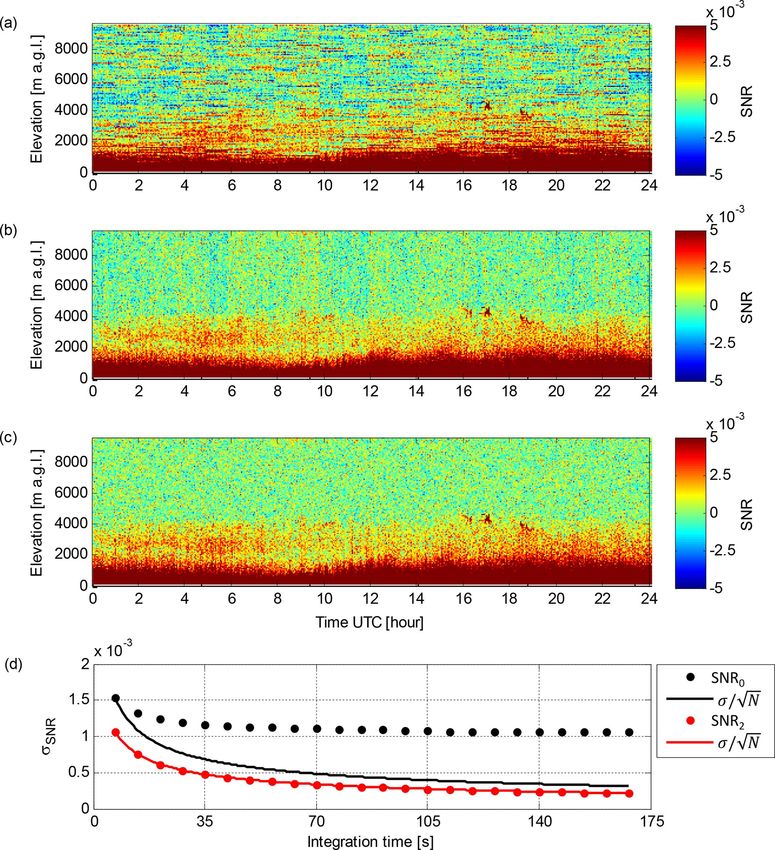
840                                             V. Vakkari et al.: A novel post-processing algorithm for Halo Doppler lidars

bution (Lothon et al., 2009), e.g vertical wind speed variance      Table 1. Specifications for Halo Doppler lidars utilised in this study.
and skewness, as well as turbulent kinetic energy dissipation
rate, Doppler lidar measurements enable the diagnosis of the            Lidar number and version      46, Stream Line
sources of turbulence within the PBL (Hogan et al., 2009;                                             53, Stream Line Pro
Harvey et al., 2013; Tuononen et al., 2017; Manninen et al.,                                          146, Stream Line XR
2018).                                                                  Wavelength                    1.5 µm
   Velocity measurements using fibre-optic Doppler lidar                Pulse repetition rate         15 kHz (46 and 53) or
                                                                                                      10 kHz (146)
systems operating at 1.5 µm wavelength depend on light scat-
                                                                        Nyquist velocity              20 m s−1
tering from aerosol particles and cloud droplets as these are
                                                                        Sampling frequency            50 MHz
small enough to behave as tracers of atmospheric motion.
                                                                        Velocity resolution           0.038 m s−1
In very clean atmospheric environments, the lack of scatter-            Points per range gate         10
ing particles becomes a limiting factor for utilising these sys-        Range resolution              30 m
tems (e.g. Manninen et al., 2016). Development of new, more             Maximum range                 9600 m (46 and 53) or
powerful yet eye-safe Doppler lidar systems has helped to                                             12 000 m (146)
overcome this limitation to a large degree (e.g. Bonin et al.,          Pulse duration                0.2 µs
2018); yet decreasing the instrumental noise level through              Lens diameter                 8 cm
post-processing of the data allows the utilisation of weaker            Lens divergence               33 µrad
signals and can lead to major improvements in data coverage             Telescope                     monostatic optic-fibre coupled
(Manninen et al., 2016). The post-processing algorithm by
Manninen et al. (2016) has the added benefit of improving
the accuracy of the signal-to-noise ratio (SNR), which leads        2    Instrumentation and measurements
to more accurate uncertainty estimates of the measured radial
velocity (Rye and Hardesty, 1993; Pearson et al., 2009). This       In this study we utilise data from three different versions
is especially important for the retrieval of turbulent properties   of Halo Photonics scanning Doppler lidars (Pearson et al.,
under weak signal conditions, as uncertainty in instrumental        2009): lidar 46 is a Stream Line system, lidar 53 is a Stream
noise level propagates into turbulent properties and wind re-       Line Pro system and lidar 146 is a Stream Line XR sys-
trievals (O’Connor et al., 2010; Vakkari et al., 2015; Newsom       tem. All Halo Photonics Stream Line versions are 1.5 µm
et al., 2017). Naturally, post-processing methods can be ap-        pulsed Doppler lidars with a heterodyne detector that can
plied to historical data sets as well.                              switch between co- and cross-polar channels (Pearson et al.,
   Here we present an improved post-processing algorithm            2009). The Stream Line and the more powerful Stream Line
for Halo Photonics Stream Line Doppler lidars, which are            XR lidars are capable of full hemispheric scanning, and the
currently widely used for PBL research (O’Connor et al.,            scanning patterns are user-configurable. The Stream Line
2010; Pearson et al., 2010; Harvey et al., 2013; Hirsikko et        Pro version is designed for harsher environmental conditions
al., 2014; Schween et al., 2014; Päschke et al., 2015; Vakkari      with no exterior moving parts, which limits the scanning to
et al., 2015; Banakh and Smalikho, 2016; Tuononen et al.,           within a cone of 20◦ from the vertical. In this study, however,
2017; Bonin et al., 2018). Building on the work by Manni-           we only utilise vertically pointing measurements in co-polar
nen et al. (2016), we show that, by changing the way instru-        mode, and thus there is no practical difference between the
mental noise level is determined during periodic background         limited and fully scanning versions.
checks, the sensitivity can be improved by as much as a fac-           The minimum range for all instruments is 90 m, and stan-
tor of 5; by averaging high time resolution data, signals with      dard operating specifications for the different versions are
an SNR as low as −32 dB can be utilised. Case studies from          given in Table 1. The telescope focus of the Stream Line and
different environments in Finland, Greece and South Africa          Stream Line Pro lidars is user-configurable between 300 m
are presented to demonstrate how the new post-processing            and infinity, whereas the Stream Line XR focus cannot be
algorithm increases data availability for turbulent retrievals      changed. Integration time per ray is user-adjustable and can
in the PBL, improves detection of high-altitude cirrus clouds       be optimised between high sensitivity (long integration time)
and enables observation of elevated aerosol layers 2 to 4 km        and high temporal resolution (short integration time) depend-
above ground level.                                                 ing on the environmental conditions and research questions.
   Next, in Sect. 2 we introduce the Halo Photonics Stream          In the measurements utilised in this study, 7 s integration time
Line, Stream Line Pro and Stream Line XR lidars used in this        is used for lidars 46 and 53, while lidar 146 is operated with
study. Section 3 describes the improved SNR post-processing         10 s integration time.
algorithm, and in Sect. 4 the three case studies are presented,        In measurement mode the Halo Doppler lidars provide
followed by concluding remarks.                                     three parameters along the beam direction: radial Doppler
                                                                    velocity (vr), SNR and attenuated backscatter (β), which is
                                                                    calculated from SNR taking into account the telescope focus.
                                                                    As part of post-processing, we calculate the measurement

Atmos. Meas. Tech., 12, 839–852, 2019                                                     www.atmos-meas-tech.net/12/839/2019/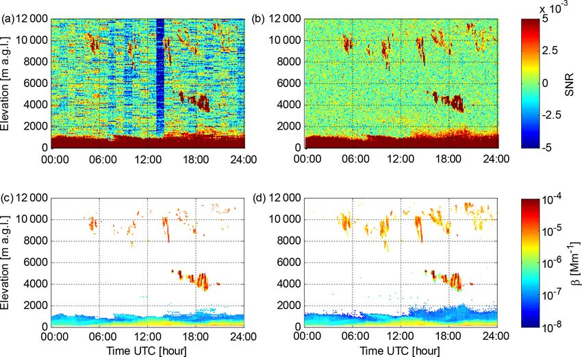
V. Vakkari et al.: A novel post-processing algorithm for Halo Doppler lidars                                                   841

uncertainty in vr (σ vr) from SNR according to O’Connor
et al. (2010). As discussed earlier, in calculating turbulent
parameters from Doppler lidar observations, accurate σ vr is
needed to differentiate turbulence from instrumental noise
(e.g. O’Connor et al., 2010; Vakkari et al., 2015; Newsom
et al., 2017).
   We present case studies of Halo Doppler lidar measure-
ments at three different locations with three different instru-
ments. Lidar 53 was deployed at Finokalia, Crete, Greece
(35.34◦ N, 25.67◦ E), on 8 July 2014. Lidar 46 was de-
ployed at Welgegund, South Africa (26.57◦ S, 26.94◦ E), on
6 September 2016 and lidar 146 was deployed at Helsinki,
Finland (60.20◦ N, 24.96◦ E), on 1 and 6 May 2018.
   Additionally, we utilise collocated Raman lidar measure-
ments at Finokalia. These measurements were carried out
using the OCEANET PollyXT multiwavelength Raman and
polarization lidar system of the Leibniz Institute for Tropo-
spheric Research (TROPOS). A detailed description of the
instrument and its measurements is provided in Engelmann et
al. (2016) and Baars et al. (2016), respectively. In brief, Pol-
lyXT operates using a Nd:YAG laser that emits light pulses
at 1064 nm with a repetition frequency of 20 Hz. The radi-
ation frequency is doubled and tripled, resulting in the si-
multaneous emission of 355, 532 and 1064 nm in the atmo-
sphere. The receiver features 12 channels that enable mea-
surements of elastically (three channels) and Raman scat-
tered light (387 and 607 channels for aerosols, 407 for water
vapour) as well as depolarisation state of the incoming light
(355 and 532 nm) and near-range measurements (two elastic
and two aerosol Raman channels). In this study, the mea-
surements at 1064 nm are used. The lidar measurements at
Finokalia were collected during the 2014 CHARacterization
of Aerosol mixtures of Dust and Marine origin experiment
(CHARADMExp) on the northern coast of Crete, Greece.               Figure 1. (a) Pbkg measured by lidar 46 on 6 September 2016 at
                                                                   23:00 UTC and Pbkg measured by lidar 146 on 1 May 2018 at
                                                                   10:00 UTC. Pfit is also indicated for both systems. (b) 2-D his-
3     Improved background check handling algorithm                 togram of mean Pbkg vs. T for lidar 46. (c) 2-D histogram of mean
                                                                   Pbkg vs. T for lidar 146.
3.1    Signal-to-noise ratio in Halo Doppler lidars

Halo Doppler lidars measure the noise level during periodic        a small linear increase with increasing distance z from the
background checks, typically once an hour, in which the            lidar (Fig. 1a); Pbkg (z) following a second-order polynomial
scanner is set to point to an internal (limited scan) or ex-       can also occur (Manninen et al., 2016). For Stream Line XR
ternal target mounted on the instrument itself (hemispheric        instruments, Pbkg (z) can vary between a linear and an inverse
scan) so that no atmospheric signal is recorded. The raw sig-      exponential shape (Fig. 1a), for which the inverse exponen-
nal from the amplifier during the background check (Pbkg )         tial Pbkg (z) can be represented as
is saved as a profile in ASCII files (“Background_ddmmyy-                           b1
HHMMSS.txt”) with the range resolution configured for              Pbkg (z) =                  ,                                (1)
                                                                                exp(b2 · zb3 )
the normal measurement mode. For most Stream Line and
Stream Line Pro firmware versions, Pbkg is written on one          where b1 , b2 and b3 are scalars and can be determined from
line with a fixed precision of six decimals but a varying field    a least-squares fit.
width for each range gate. In Stream Line XR firmware, the            In Stream Line and Stream Line Pro lidars, the magnitude
Pbkg value at each range gate is written on its own line.          of Pbkg increases non-linearly with instrument internal tem-
   In most Stream Line and Stream Line Pro instruments,            perature (T ) (Fig. 1b). For Stream Line XR lidars, which
the profile Pbkg (z) is flat (constant with range) or presents     use a different amplifier, the mean Pbkg does not depend

www.atmos-meas-tech.net/12/839/2019/                                                      Atmos. Meas. Tech., 12, 839–852, 2019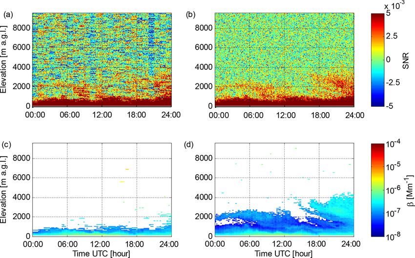
842                                               V. Vakkari et al.: A novel post-processing algorithm for Halo Doppler lidars

on T ; however, the amplifier alternates randomly between              to Pbkg (z). Furthermore, knowing the typical noise level of a
a high mode (Pbkg ≈ 3.6×10⁸ for lidar 146) and a low mode              certain instrument, a rms threshold can be applied to discard
(Pbkg ≈ 3.2 × 10⁸ for lidar 146) as seen in Fig. 1c. Further-          bad fits and to flag periods of increased uncertainty.
more, it appears that the inverse exponential Pbkg shape only             Denoting the selected fit to Pbkg (z) as Pfit (z), the residual
occurs in the low mode, but not all low-mode Pbkg profiles             is
follow Eq. (1).
   The Halo Doppler lidar firmware accounts for changes in             Pbkg,res (z) = Pbkg (z) − Pfit (z).                           (3)
Pbkg level by calculating SNR as
                                                                       Averaging Pbkg,res (z) over a large number of Pbkg (z) pro-
        A0 · P0 (z)                                                    files reveals a persistent structure in the residual (Fig. 2a).
SNR0 =                 − 1,                                     (2)
       Abkg · Pbkg (z)                                                 This part of Pbkg,res (z) originates in the amplifier response
                                                                       to the transmitted pulse, denoted here as Pamp (z), and it is
where P0 (z) is the raw signal from the amplifier during each          the main reason for using the gate-by-gate defined Pbkg (z)
measurement, Pbkg (z) has been obtained during the previous            profile in SNR calculation by the manufacturer. However,
background check and scalar scaling factors A0 and Abkg are            Pamp (z) stays reasonably constant over time and can be ob-
determined online for each P0 andPbkg profile. Here, we de-            tained from a long enough data set of Pbkg (z). Here, we used
note the unprocessed SNR output by the instrument as SNR0 .            a discrete wavelet transform with a Symmlet order 8 wavelet
Note that A0 and Abkg are not saved by the firmware, which             as a low-pass filter to de-noise the averaged Pbkg,res (z). As
means that the high and low mode in Stream Line XR lidars              shown in Fig. 2a, Pamp (z) is instrument-specific and needs to
cannot be identified in the SNR0 time series.                          be determined individually for each device.
   Equation (2) is straightforward to determine online as                 In Stream Line and Stream Line Pro lidars, T has a small
there are no assumptions about the shape of Pbkg , and it gives        effect on Pamp (z) as seen in Fig. 2b. However, this can be
a reasonably good first estimate of SNR. However, Eq. (2)              addressed based on a suitably long T data set and Pbkg,res (z)
is vulnerable to inaccuracy in determining A0 and Abkg as              by determining Pamp (z) as a function of the internal temper-
well as to any deviation from the actual noise level during            ature. In practice, at least 300 Pbkg (z) profiles are required
measurement of Pbkg . An offset in A0 inflicts a constant off-         to obtain a reliable estimate of Pamp (z). Consequently, for an
set in SNR0 in a single profile, while an offset in Abkg does          11-month measurement campaign at Welgegund, we could
the same for all profiles between two background checks (cf.           determine Pamp as a function of T at 1 ◦ C resolution from
Manninen et al., 2016). The magnitude of typical offsets in            25 to 31 ◦ C (Fig. 2b). For T < 23 ◦ C or T > 35 ◦ C we could
A0 and Abkg varies from instrument to instrument; in some              only determine aggregate Pamp profiles, but then these tem-
cases they can have a major effect on data coverage (Manni-            perature ranges comprise only 9 % of the measurements in
nen et al., 2016).                                                     this data set. For optimal data quality, additional temperature
   In all Halo Doppler lidars Pbkg contains a small but vary-          stabilisation could be applied to ensure that Pamp is always
ing offset from the actual noise level at each range gate be-          in the well-characterised temperature range.
cause of the finite duration of the background check. These               In Stream Line XR lidars, Pamp does not depend on T ;
offsets appear as a small constant offset in SNR0 at each              however, Pamp has to be determined separately for the high
range gate between two background checks. To minimise the              and low mode of Pbkg (see Fig. 1c). For lidar 146, we define
effect of offset in Pbkg , the integration time of background          Pbkg high mode as mean Pbkg > 3.4×10⁸ and Pbkg low mode
check measurement was originally designed to be 6 times as             as mean Pbkg < 3.4 × 10⁸ , respectively. As seen in Fig. 2c,
long as the integration time in measurement mode. The dura-            Pamp for these two modes differs substantially.
tion of the background check is user-configurable; however,               We consider the sum of Pfit (z) and Pamp (z) as the best es-
for long integration times of up to 6 min considered in this           timate for the actual instrumental noise level during a back-
paper such long background checks are not a viable option.             ground check:
In the next section we present an improved algorithm to cor-
rect SNR0 for inaccuracies in A0 , Abkg and Pbkg .                     Pnoise (z) = Pfit (z) + Pamp (z).                             (4)
3.2   Improved SNR post-processing algorithm                           Using Eq. (2), we can move from a Pbkg -based SNR (i.e.
                                                                       SNR0 ) to a Pnoise -based, corrected SNR (denoted here as
Whether Pbkg (z) is linear or follows some other functional
                                                                       SNR1 ) simply as
form is readily determined by fitting expected functions to it
(cf. Manninen et al., 2016). For Stream Line and Stream Line                                           Pbkg (z)
Pro lidars we consider a second-order polynomial to repre-             SNR1 (z) = (SNR0 (z) + 1) ·                − 1.               (5)
                                                                                                       Pnoise (z)
sent Pbkg (z) better than a linear fit if it has at least 10 % lower
root-mean-squared (rms) error than the linear fit to Pbkg (z).         Next, we utilise the Manninen et al. (2016) algorithm to iden-
For Stream Line XR we consider Eq. (1) to represent Pbkg (z)           tify any possible bias in the A0 to Abkg ratio. In short, Man-
better if it has at least 5 % lower rms error than the linear fit      ninen et al. (2016) cloud and aerosol screening is applied

Atmos. Meas. Tech., 12, 839–852, 2019                                                      www.atmos-meas-tech.net/12/839/2019/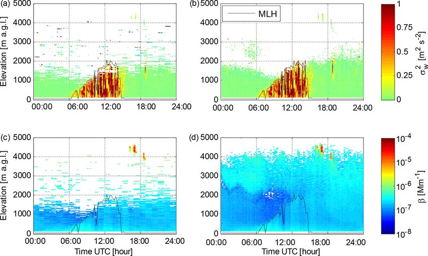
V. Vakkari et al.: A novel post-processing algorithm for Halo Doppler lidars                                                          843

                                                                        which is our final corrected SNR.
                                                                           Note that to correct only for the bias in the A0 to Abkg
                                                                        ratio, a scalar denominator in Eq. (6) would be sufficient.
                                                                        However, using the fitted profile SNRfit (z) as the denomina-
                                                                        tor accounts for possible changes in the slope of Pnoise since
                                                                        the last background check.

                                                                        3.2.1   Implications for Stream Line XR lidars

                                                                        The calculation of SNR2 with Eq. (6) relies on the fitting
                                                                        to cloud- and aerosol-free measurements. For Stream Line
                                                                        and Stream Line Pro lidars, which do not exhibit the inverse
                                                                        exponential Pbkg shape, SNRfit (z) will capture the shape
                                                                        of the actual noise level in nearly all cases. However, for
                                                                        Stream Line XR lidars the randomly occurring inverse ex-
                                                                        ponential Pbkg (z) shape (Fig. 1a) is almost always masked
                                                                        by aerosol and/or cloud signal during measurement. Thus, it
                                                                        is not possible to correct for changes in shape of Pnoise (z)
                                                                        with SNRfit (z) during post-processing. However, the magni-
                                                                        tude of uncertainty in Pnoise (z) can be estimated from the av-
                                                                        erage depth of the inverse exponential dip in Pbkg (z) during
                                                                        background checks (see Fig. 3a).
                                                                            Now as A0 is not saved, it is not possible to tell whether the
                                                                        amplifier was operating in high or low mode during measure-
                                                                        ment. Consequently, the difference in Pamp for the amplifier
                                                                        high and low modes also adds to the uncertainty in SNR for
                                                                        Stream Line XR systems, but, compared to the effect of the
                                                                        inverse exponential shape of Pbkg (z), the effect of Pamp is ap-
                                                                        proximately 10 times smaller. However, any possible bias in
                                                                        the A0 to Abkg ratio can be corrected, and this is readily done
                                                                        by applying a linear fit to SNR1 (z) at range gates 100–400
                                                                        (for which SNR is not affected by inverse exponential Pbkg )
                                                                        and using this as SNRfit (z) in Eq. (6).
Figure 2. (a) Lidar 46 Pbkg,res averaged from 20 August 2016 to
                                                                            In practice, there are two options for SNR post-processing
14 June 2017 (7193 background checks). Lidar 53 Pbkg,res averaged
from 1 January 2014 to 30 November 2015 (16 802 background              for Stream Line XR lidars. The first option is to accept the
checks). Pamp is plotted for both systems. (b) First 100 range gates    fitted Eq. (1) for Pfit (z) when it describes Pbkg (z) better. With
of lidar 46 Pamp calculated for different ranges of T . (c) Lidar 146   this approach SNR2 may overestimate the actual SNR if the
Pbkg,res averaged from 12 January to 31 May 2018. Pbkg,res is aver-     shape of Pnoise changes from Eq. (1) to being linear after the
aged separately for high Pbkg mode (1375 background checks) and         background check. Correspondingly, a change from a linear
for low Pbkg mode (1623 background checks). Pamp is plotted for         Pnoise to the inverse exponential shape during measurement
both modes.                                                             results in SNR2 underestimating the actual SNR.
                                                                            The second option for Stream Line XR SNR post-
                                                                        processing is to calculate a linear fit to Pbkg (z) based on
first to time series of SNR1 . Note that typically cloud and            range gates 100–400 and to always use this for Pfit (z). In
aerosol signal is easier to discern in SNR1 than in SNR0 , and          this case, we only use high-mode Pamp (z) in calculating the
thus cloud screening is applied after Eq. (5). Then, first- and         noise level (Eq. 4) and denote it as Pnoise0   (z). Consequently
second-order polynomial fits are calculated for each cloud-                   0
                                                                        SNR 2 is the lower limit of the actual SNR, which can be
screened profile of SNR1 (z), and a rms threshold is used to            useful if an SNR threshold is used to determine the usable
select the appropriate fit, similar to determining Pfit (z). De-        signal for further analysis. For lidar 146 background checks
noting the selected fit to cloud- and aerosol-free measure-             from 12 January to 31 May 2018, the underestimation was
ments as SNRfit (z) we obtain                                           on average 0.5 % of SNR+1 at the first usable range gate
                                                                        and decreased rapidly with increasing range (Fig. 3a). In the
              SNR1 (z) + 1                                              worst case, the underestimation at the first usable range gate
SNR2 (z) =                   − 1,                                (6)    was 3 % of SNR+1.
              SNRfit (z) + 1

www.atmos-meas-tech.net/12/839/2019/                                                         Atmos. Meas. Tech., 12, 839–852, 2019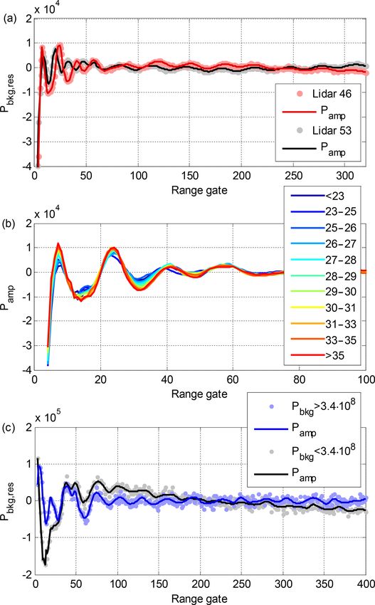
844 V. Vakkari et al.: A novel post-processing algorithm for Halo Doppler lidars
0
Figure 3. (a) 2-D histogram of the ratio of Pnoise (z) (best estimate) to Pnoise (z) (linear fit only) for lidar 146 background checks. The mean
of the ratio is also indicated. (b) σvr as a function of SNR for lidar 146.
Uncertainty in SNR leads to uncertainty in σvr , as σvr is become visible as vertical stripes, for instance between 05:00
mostly a function of SNR (Pearson et al., 2009). However, and 06:00 UTC in Fig. 4b, which are then corrected for in the
σvr decreases rapidly with increasing SNR (Fig. 3b). There- time series of SNR2 (Fig. 4c).
fore, even the worst-case underestimation in SNR only has a Comparing the standard deviation of SNR (σSNR ) for
limited effect on σvr if SNR is even moderately high (> 0.03, cloud- and aerosol-free range gates shows a clear improve-
−15.2 dB). On the other hand, for observations > 2000 m ment in the noise level with the new post-processing al-
away from the lidar, where signals are typically low, the un- gorithm (Fig. 4d). The main advantage of the new post-
certainty in SNR is also low (Fig. 3a). In the end, uncertainty processing algorithm is that it enables averaging SNR; for
in SNR and its effects in β and σvr need to be evaluated indi- SNR0 any offsets in Pbkg (z) become the limiting factor. This
vidually for each profile in Stream Line XR lidars. is clearly seen in Fig. 4d, which shows σSNR for SNR2 de-
creases√with increasing integration time per profile following
the σ/ N rule closely as expected, but increasing integra-
4 Case studies tion time has little effect on σSNR for SNR0 .
Figure 5 demonstrates how the lower noise floor with the
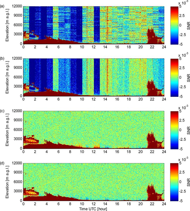
4.1 Welgegund 6 September 2016 new post-processing algorithm allows vertical wind speed
variance (σw2 ) up to 2000 m a.g.l. (i.e. up to the top of the
On 6 September 2016 lidar 46 was operating at Welgegund,
mixed layer) to be determined on this day. Furthermore, by
South Africa, and a time series of SNR in vertically point-
averaging the originally 7 s data to 168 s integration time per
ing measurement mode for this day is presented in Fig. 4. In
profile and applying the new post-processing algorithm, the
this case, SNR0 is very close to 0 when there are no clouds
SNR threshold at the 3σ level (see Fig. 4d) can be decreased
or aerosol present (Fig. 4a), indicating that the online cal-
from 0.0032 (−25 dB) for SNR0 to 0.00065 (−32 dB) for
culation of A0 and Abkg is quite successful. However, the
SNR2 . Consequently, β can be retrieved for the elevated
presence of small but varying offsets in Pbkg (z) is apparent
aerosol layer at 2000–4000 m a.g.l. (Fig. 5c, d). Note that the
in Fig. 4a as horizontal stripes in SNR0 time series between
offsets in Pbkg (z) result in horizontal stripes in the 168 s in-
the background checks conducted on the hour.
tegration time β calculated from SNR0 in Fig. 5c.
In the SNR1 time series (Fig. 4b) the horizontal stripes
A lower noise floor also enables wind retrievals with a
have been removed by applying the smooth Pnoise -based
lower SNR threshold, which increases the data availabil-
background using Eq. (5). At the same time, the elevated
ity. The effect on data availability depends on atmospheric
aerosol layer at 2000–4000 m above ground level (a.g.l.) be-
conditions, though. In this case for instance (Welgegund,
comes easily discernible. Small biases in the A0 to Abkg ratio
Atmos. Meas. Tech., 12, 839–852, 2019 www.atmos-meas-tech.net/12/839/2019/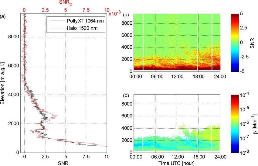
V. Vakkari et al.: A novel post-processing algorithm for Halo Doppler lidars                                                              845

Figure 4. Data from lidar 46 at Welgegund on 6 September 2016. (a) Time series of the SNR0 profile in vertically pointing mode. (b) Time
series of the SNR1 profile in vertically pointing mode. (c) Time series of the SNR2 profile in vertically
                                                                                                    √     pointing mode. (d) σSNR as a function
of integration time per profile for SNR0 and SNR2 for range gates at 4800–9000 m a.g.l. Also σ/ N, where σ is σSNR at an integration time
of 7 s (original integration time per profile) and N is the number of averaged profiles, is included in (d).

6 September 2016), a 75◦ elevation angle velocity azimuth                 determination of the instrumental uncertainty in wind re-
display (VAD) scan was utilised for horizontal wind retrieval             trievals. However, as a major fraction of the uncertainty in
every 15 min. With the new post-processing algorithm, the                 retrieved winds arises in atmospheric turbulence (Newsom et
SNR threshold for wind retrieval could be decreased from                  al., 2017), the more accurate SNR will only have a limited
0.0045 to 0.0032. This decrease in the SNR threshold en-                  effect on the overall uncertainty in the wind retrieval. There-
abled the wind retrieval for 2–13 range gates more from each              fore, the uncertainty in each wind retrieval should be eval-
VAD scan; on average, winds could be determined from 7.5                  uated, e.g. with the methodology of Newsom et al. (2017),
additional range gates per VAD scan. That is, vertical cov-               before the wind retrievals are disseminated.
erage of wind retrievals increased on average by 200 m with
the new post-processing.                                                  4.2   Helsinki 1 and 6 May 2018
   Wind retrievals at lower SNR will have higher uncer-
tainty due to higher instrumental noise in radial velocity                Measurements using lidar 146 at Helsinki, Finland, on
measurement; yet enhanced SNR will enable more accurate                   6 May 2018 (Fig. 6) present all the issues with a Stream Line

www.atmos-meas-tech.net/12/839/2019/                                                            Atmos. Meas. Tech., 12, 839–852, 2019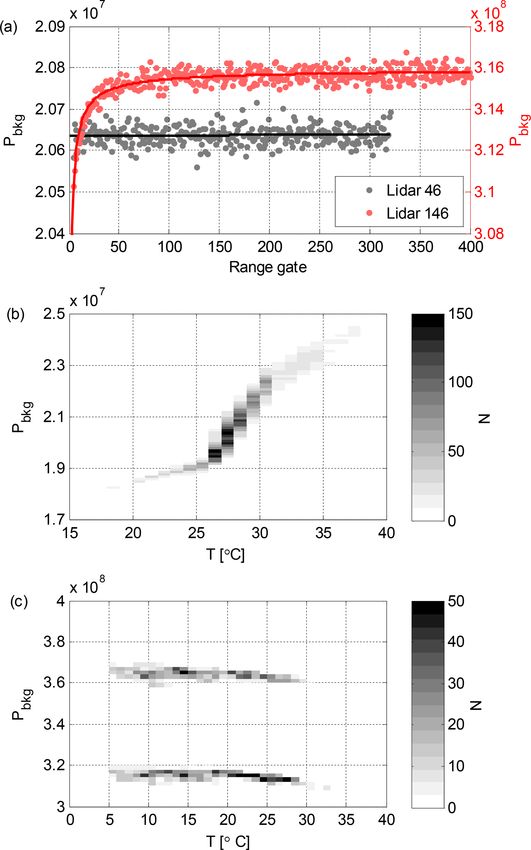
846                                                V. Vakkari et al.: A novel post-processing algorithm for Halo Doppler lidars

Figure 5. Data from lidar 46 at Welgegund on 6 September 2016. (a) Time series of the σw2 profile, for which a threshold of 0.0031 (2σ ) has
been applied to SNR0 . (b) Time series of the σw2 profile, for which a threshold of 0.0021 (2σ ) has been applied to SNR2 . In (a) and (b) the
instrumental noise contribution to σw2 has been subtracted. (c) Time series of β obtained with 168s integration time from SNR0 ; β has been
filtered with a threshold of 0.0032 (3σ ) applied to SNR0 . (d) Time series of β obtained with 168 s integration time from SNR2 ; β has been
filtered with a threshold of 0.00065 (3σ ) applied to SNR2 . Mixing layer height (MLH) determined from panels (b) and (d) is also indicated.

XR lidar at its worst. In Fig. 6a, SNR0 is negative, e.g. from           Fig. 7a. On this day there are cirrus clouds present at 8000–
01:00 to 05:00, 06:00 to 10:00 and 12:00 to 13:00 UTC be-                12 000 m a.g.l., but the stripes due to offsets in Pbkg (z) make
cause of an erroneous Abkg coefficient. On the other hand,               it difficult to distinguish the clouds from noise in SNR0 .
the individual profiles with unrealistically high SNR0 around            Applying the new post-processing algorithm and increasing
11:00, 14:00 to 15:00 and 20:00 to 21:00 UTC indicate er-                integration time from 10 to 60 s for this day enables the
rors in the A0 coefficient. Additionally, horizontal stripes in          SNR threshold at the 3σ level to be lowered from 0.0035
SNR0 time series similar to lidar 46 (Fig. 4a) indicate off-             (−24.5 dB) for SNR0 to 0.0012 (−29 dB) for SNR2 . This re-
sets in Pbkg (z). The reason for poor determination of A0 and            sults in a significant increase in data coverage for the cirrus
Abkg for lidar 146 seems to be that Pbkg (z) is frequently non-          clouds, as shown in Fig. 7c and d.
linear, unlike for lidar 46, for example.
   The new post-processing algorithm corrects the errors                 4.3    Finokalia 8 July 2014
in A0 and Abkg as well as the stripes due to offsets in
Pbkg (z) as seen in Fig. 6c. However, Fig. 6c shows that                 Time series of SNR in vertically pointing mode with lidar 53
Pbkg (z) changing between the inverse exponential and lin-               on 8 July 2014 at Finokalia, Greece, are presented in Fig. 8.
ear shape causes over- and underestimation of SNR2 in the                On this day, SNR0 is close to 0 for 4000–9600 m a.g.l. el-
lowest 1500 m a.g.l. For instance, positive SNR2 in the low-             evation (Fig. 8a), indicating that the online calculation of
est 1000 m at 12:00 to 13:00 UTC and negative SNR2 in the                A0 and Abkg is quite successful. Only at 00:00–01:00 and
lowest 1000 m at 14:00 to 15:00 UTC are due to noise level               20:00–21:00 UTC is SNR0 negative, indicating a small offset
shape changes between background check and measurement                   in Abkg . However, horizontal stripes in the SNR0 time series
modes. During these periods, the lidar signal is fully atten-            between the background checks are apparent in Fig. 8a, indi-
uated by a cloud within the lowest 200 m, and consequently               cating the presence of small but varying offsets in Pbkg (z).
SNR2 in the 200–1000 m range should be zero. In Fig. 6d,                    After SNR post-processing (Fig. 8b), elevated aerosol lay-
SNR0 2 is only calculated using a linear fit to Pbkg (z) as dis-         ers at 1000–4000 m a.g.l. are clearly visible on this day.
cussed in Sect. 3.2.1. This removes the overestimate of SNR              These aerosol layers were also observed with a co-located
at 12:00–13:00 UTC, but cannot correct the underestimates.               multiwavelength Raman lidar, Polly XT (Baars et al., 2016;
   Measurements with lidar 146 on 1 May 2018 at Helsinki                 Engelman et al., 2016). A comparison of lidar 53 and the
present much less noisy SNR0 than on 6 May 2018, as seen in              Raman lidar measurements at 1064 nm wavelength is pre-
                                                                         sented in Fig. 9. Considering the wavelength difference, the

Atmos. Meas. Tech., 12, 839–852, 2019                                                         www.atmos-meas-tech.net/12/839/2019/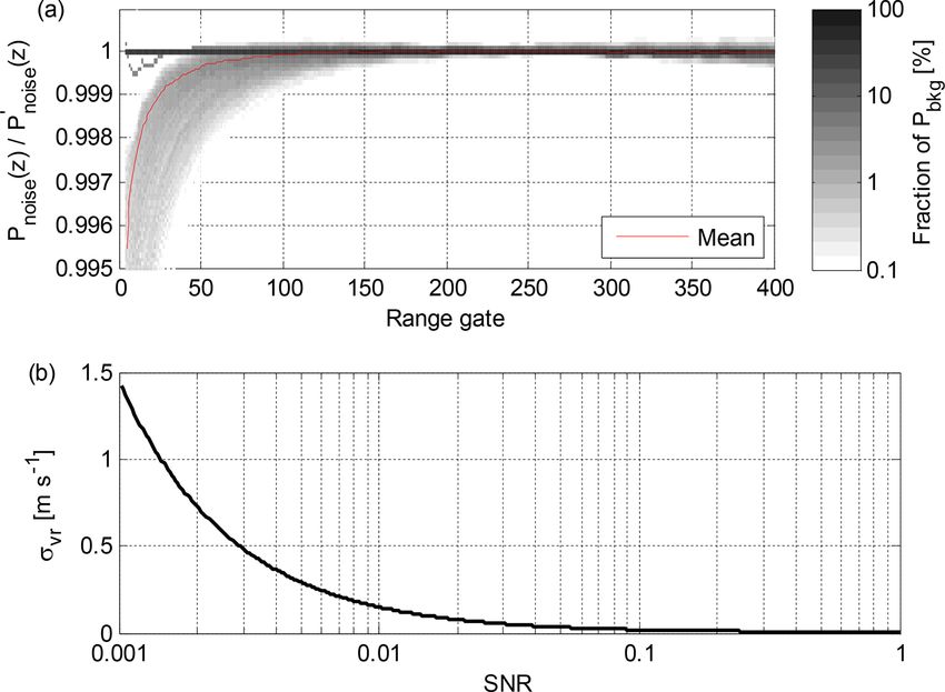
V. Vakkari et al.: A novel post-processing algorithm for Halo Doppler lidars                                                           847

Figure 6. Data from lidar 146 at Helsinki on 6 May 2018. (a) Time series of the SNR0 profile in vertically pointing mode. (b) Time series of
the SNR1 profile in vertically pointing mode. (c) Time series of the SNR2 profile in vertically pointing mode. (d) Time series of the SNR0 2
(always based on a linear fit to Pbkg (z)) profile in vertically pointing mode.

agreement between the two systems is reasonably good. Fur-              Line and Stream Line Pro lidars, this method enables accu-
ther averaging of SNR2 , in this case up to 350 s integration           rate SNR and β retrievals from the first usable gate onwards.
time, allows the determination of β for the elevated aerosol            For Stream Line XR lidars, we identified a previously un-
layers. With this long integration time we can reach a 3σ               known source of uncertainty in the near-range (< 1500 m)
SNR threshold of 0.00059 (−32 dB) for SNR2 . For SNR0 ,                 SNR due to variations in the noise floor of these systems. We
offsets in Pbkg (z) are the limiting factor in determining the          present a method to estimate the magnitude of this source of
SNR threshold, and at the 3σ level only 0.0044 (−24 dB)                 uncertainty, although it cannot be completely eliminated.
can be achieved.                                                           We have shown that defining the noise floor on a point-
                                                                        by-point basis during periodic background checks results in
                                                                        a small, variable offset in SNR at each range gate. This off-
5   Conclusions                                                         set is due to finite duration of the background check and be-
                                                                        comes the limiting factor in retrieving weaker signals with
In this paper we have presented an improved SNR post-                   Halo Doppler lidars, or with any system based on such a
processing algorithm for Halo Doppler lidars. For Stream

www.atmos-meas-tech.net/12/839/2019/                                                          Atmos. Meas. Tech., 12, 839–852, 2019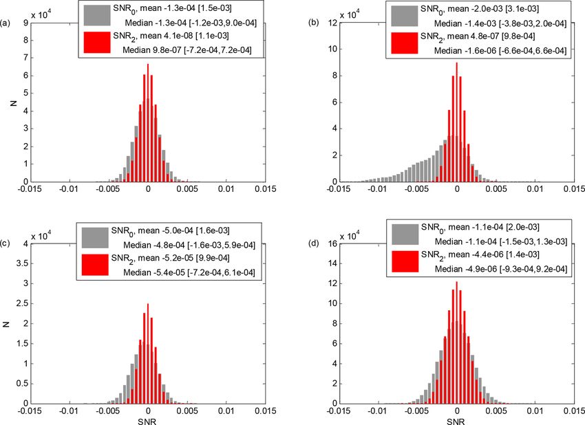
848                                                V. Vakkari et al.: A novel post-processing algorithm for Halo Doppler lidars

Figure 7. Data from lidar 146 at Helsinki on 1 May 2018. (a) Time series of the SNR0 profile in vertically pointing mode. (b) Time series of
the SNR2 profile in vertically pointing mode. (c) Time series of β obtained with 60 s integration time from SNR0 ; β has been filtered with
a threshold of 0.0035 (3σ ) applied to SNR0 . (d) Time series of β obtained with 60 s integration time from SNR2 ; β has been filtered with a
threshold of 0.0012 (3σ ) applied to SNR2 .

Figure 8. Data from lidar 53 at Finokalia on 8 July 2014. (a) Time series of the SNR0 profile in vertically pointing mode. (b) Time series of
the SNR2 profile in vertically pointing mode. (c) Time series of β obtained with 350 s integration time from SNR0 ; β has been filtered with
a threshold of 0.0044 (3σ ) applied to SNR0 . (d) Time series of β obtained with 350 s integration time from SNR2 ; β has been filtered with a
threshold of 0.00059 (3σ ) applied to SNR2 .

Atmos. Meas. Tech., 12, 839–852, 2019                                                         www.atmos-meas-tech.net/12/839/2019/
V. Vakkari et al.: A novel post-processing algorithm for Halo Doppler lidars                                                            849

Figure 9. (a) Vertical profiles of SNR from PollyXT at 1064 nm wavelength and SNR2 from lidar 53 at Finokalia on 8 July 2014. Both
profiles are obtained at 21:00 UTC; the integration time of the lidar 53 profile is 350 s, and the integration time of the PollyXT profile is
360 s. (b) Time series of PollyXT SNR at 1064 nm wavelength with 360 s integration time at Finokalia on 8 July 2014. (c) Time series of
PollyXT attenuated backscatter at 1064 nm wavelength with 360 s integration time at Finokalia on 8 July 2014.

point-by-point-defined noise floor. The improved SNR post-                  We have demonstrated that the improved SNR post-
processing algorithm removes this source of error by intro-              processing can help to retrieve turbulent properties up to
ducing a more accurate, continuous noise floor. Independent              the top of the mixed layer under low aerosol load. With en-
of the noise floor, online scaling of raw signal from the am-            hanced SNR, the instrumental noise contribution to radial ve-
plifier by the firmware fails occasionally. This source of er-           locity variance can be estimated with better accuracy, which
ror in SNR was targeted by Manninen et al. (2016), and                   will improve the quality of turbulent parameter retrievals.
their algorithm is adapted here as part of the improved SNR              The reduced noise floor enables horizontal wind retrievals
post-processing algorithm (Eq. 6). Correcting for these two              with a lower SNR threshold and increases data availabil-
sources of error in SNR enables data to be retrieved at much             ity, depending on atmospheric conditions. Furthermore, we
lower SNR than before. By increasing integration time per                have demonstrated that a combination of reduced noise floor
profile to a few minutes, SNR down to 6 × 10⁻⁵ (−32 dB)                  and increased integration time allows detection of elevated
can be utilised.                                                         aerosol layers with Stream Line and Stream Line Pro lidars.
   Our analysis shows that even if the technical specifications          Even for the more powerful Stream Line XR lidars, the new
of two Doppler lidar systems are identical, their instrumental           SNR post-processing can increase data availability, e.g. in
noise characteristics can be quite different (Fig. 2). There-            the case of high-altitude cirrus clouds. In conclusion, the
fore, the lidar operator should inspect each system individ-             improved SNR post-processing introduced in this paper en-
ually to ensure the highest data quality. Note that this algo-           hances the capabilities of Halo Doppler lidars in studying at-
rithm or similar processing is needed to define the instrumen-           mospheric turbulence in weak signal conditions and opens up
tal noise level even if raw spectra are utilised instead of the          new possibilities for studying elevated aerosol layers, such as
processed data. The algorithm presented here can be applied              volcanic ash, Aeolian dust or biomass burning smoke.
in semi-operational use as long as at least 300 background
checks (acquired in 2 weeks of measurements with typical
configuration) are available for characterising the amplifier            Data availability. Doppler lidar data are available upon request to
response to the transmitted pulse. A MATLAB implementa-                  the corresponding author. Raman lidar data are available upon re-
tion of this algorithm is available through GitHub (Manni-               quest to polly@tropos.de.
nen, 2019).

www.atmos-meas-tech.net/12/839/2019/                                                           Atmos. Meas. Tech., 12, 839–852, 2019
850                                            V. Vakkari et al.: A novel post-processing algorithm for Halo Doppler lidars

Appendix A

Figure A1. Histograms of SNR0 and SNR2 in a cloud- and aerosol-free regime for the four case studies considered in Sect. 4. For each
case, mean [standard deviation] and median [25th, 75th percentile] of SNR0 and SNR2 are included. (a) Welgegund on 6 September 2016,
00:00–24:00 UTC, 4800–9000 m a.g.l. (b) Kumpula on 1 May 2018, 02:00–24:00 UTC, 6000–12 000 m a.g.l. (c) Kumpula on 6 May 2018,
00:00–12:00 UTC, 4000–7000 m a.g.l. (d) Finokalia on 8 July 2014, 00:00–24:00 UTC, 5000–96 000 m a.g.l.

Atmos. Meas. Tech., 12, 839–852, 2019                                                   www.atmos-meas-tech.net/12/839/2019/
V. Vakkari et al.: A novel post-processing algorithm for Halo Doppler lidars                                                            851

Competing interests. The authors declare that they have no conflict       Composite Fuzzy Logic Approach, J. Atmos. Ocean. Tech., 35,
of interest.                                                              473–490, https://doi.org/10.1175/JTECH-D-17-0159.1, 2018.
                                                                        Emeis, S., Schäfer, K., and Münkel, C.: Surface-based remote sens-
                                                                          ing of the mixing-layer height – a review, Meteorol. Z., 17, 621–
Acknowledgements. We gratefully acknowledge financial support             630, 2008.
by TOPROF (COST Action ES1303) and North-West University                Engelmann, R., Kanitz, T., Baars, H., Heese, B., Althausen, D.,
for measurements at Welgegund. CHARADMExp was an exper-                   Skupin, A., Wandinger, U., Komppula, M., Stachlewska, I. S.,
imental campaign of the National Observatory of Athens (NOA)              Amiridis, V., Marinou, E., Mattis, I., Linné, H., and Ansmann,
and was supported by the ESA-ESTEC project “Characterization              A.: The automated multiwavelength Raman polarization and
of Aerosol mixtures of Dust And Marine origin”, contract no.              water-vapor lidar PollyXT: the neXT generation, Atmos. Meas.
IPL-PSO/FF/lf/14.489. We acknowledge Ronny Engelmann and                  Tech., 9, 1767–1784, https://doi.org/10.5194/amt-9-1767-2016,
Holger Baars from TROPOS for providing Raman lidar data                   2016.
and financial support through the High-Definition Clouds and            Garratt, J.: Review: the atmospheric boundary layer, Earth-Sci.
Precipitation for advancing Climate Prediction research program           Rev., 37, 89–134, https://doi.org/10.1016/0012-8252(94)90026-
(HD(CP)2; FKZ: 01LK1209C and 01LK1212C), funded by the                    4, 1994.
Federal Ministry of Education and Research in Germany (BMBF),           Harvey, N. J., Hogan, R. J., and Dacre, H. F.: A method to diagnose
ACTRIS under grant agreement no. 262254 of the European Union             boundary-layer type using Doppler lidar, Q. J. Roy. Meteor. Soc.,
Seventh Framework Programme (FP7/2007-2013) and ACTRIS-2                  139, 1681–1693, https://doi.org/10.1002/qj.2068, 2013.
under grant agreement no. 654109 of the European Union’s                Hirsikko, A., O’Connor, E. J., Komppula, M., Korhonen, K.,
Horizon 2020 research and innovation programme.                           Pfüller, A., Giannakaki, E., Wood, C. R., Bauer-Pfundstein, M.,
                                                                          Poikonen, A., Karppinen, T., Lonka, H., Kurri, M., Heinonen,
Edited by: Ulla Wandinger                                                 J., Moisseev, D., Asmi, E., Aaltonen, V., Nordbo, A., Rodriguez,
Reviewed by: two anonymous referees                                       E., Lihavainen, H., Laaksonen, A., Lehtinen, K. E. J., Laurila,
                                                                          T., Petäjä, T., Kulmala, M., and Viisanen, Y.: Observing wind,
                                                                          aerosol particles, cloud and precipitation: Finland’s new ground-
                                                                          based remote-sensing network, Atmos. Meas. Tech., 7, 1351–
                                                                          1375, https://doi.org/10.5194/amt-7-1351-2014, 2014.
References                                                              Hogan, R. J., Grant, A. L., Illingworth, A. J., Pearson, G. N., and
                                                                          O’Connor, E. J.: Vertical velocity variance and skewness in clear
Baars, H., Kanitz, T., Engelmann, R., Althausen, D., Heese,               and cloud-topped boundary layers as revealed by Doppler lidar,
  B., Komppula, M., Preißler, J., Tesche, M., Ansmann, A.,                Q. J. Roy. Meteor. Soc. A, 135, 635–643, 2009.
  Wandinger, U., Lim, J.-H., Ahn, J. Y., Stachlewska, I. S.,            Lothon, M., Lenschow, D. H., and Mayor, S. D.: Doppler lidar mea-
  Amiridis, V., Marinou, E., Seifert, P., Hofer, J., Skupin, A.,          surements of vertical velocity spectra in the convective planetary
  Schneider, F., Bohlmann, S., Foth, A., Bley, S., Pfüller, A., Gian-     boundary layer, Bound.-Lay. Meteorol., 132, 205–226, 2009.
  nakaki, E., Lihavainen, H., Viisanen, Y., Hooda, R. K., Pereira,      Manninen, A: HALO lidar toolbox, GitHub, available at:
  S. N., Bortoli, D., Wagner, F., Mattis, I., Janicka, L., Markowicz,     https://github.com/manninenaj/HALO_lidar_toolbox (last ac-
  K. M., Achtert, P., Artaxo, P., Pauliquevis, T., Souza, R. A. F.,       cess: 16 January 2019), 2019.
  Sharma, V. P., van Zyl, P. G., Beukes, J. P., Sun, J., Rohwer, E.     Manninen, A. J., O’Connor, E. J., Vakkari, V., and Petäjä, T.: A gen-
  G., Deng, R., Mamouri, R.-E., and Zamorano, F.: An overview of          eralised background correction algorithm for a Halo Doppler li-
  the first decade of PollyNET: an emerging network of automated          dar and its application to data from Finland, Atmos. Meas. Tech.,
  Raman-polarization lidars for continuous aerosol profiling, At-         9, 817–827, https://doi.org/10.5194/amt-9-817-2016, 2016.
  mos. Chem. Phys., 16, 5111–5137, https://doi.org/10.5194/acp-         Manninen, A. J., Marke, T., Tuononen, M., and O’Connor,
  16-5111-2016, 2016.                                                     E. J.: Atmospheric Boundary Layer Classification with
Baklanov, A. A., Grisogono, B., Bornstein, R., Mahrt, L., Zilitinke-      Doppler Lidar, J. Geophys. Res.-Atmos., 123, 8172–8189,
  vich, S. S., Taylor, P., Larsen, S. E., Rotach, M. W., and Fer-         https://doi.org/10.1029/2017JD028169, 2018.
  nando, H. J. S.: The Nature, Theory, and Modeling of Atmo-            Marke, T., Crewell, S., Schemann, V., Schween, J. H., and
  spheric Planetary Boundary Layers, B. Am. Meteorol. Soc., 92,           Tuononen, M.: Long-Term Observations and High-Resolution
  123–128, https://doi.org/10.1175/2010BAMS2797.1, 2011.                  Modeling of Midlatitude Nocturnal Boundary Layer Processes
Banakh, V. A. and Smalikho, I. N.: Lidar observations of atmo-            Connected to Low-Level Jets, J. Appl. Meteorol. Clim., 57,
  spheric internal waves in the boundary layer of the atmosphere          1155–1170, https://doi.org/10.1175/JAMC-D-17-0341.1, 2018.
  on the coast of Lake Baikal, Atmos. Meas. Tech., 9, 5239–5248,        Newsom, R. K., Brewer, W. A., Wilczak, J. M., Wolfe, D. E.,
  https://doi.org/10.5194/amt-9-5239-2016, 2016.                          Oncley, S. P., and Lundquist, J. K.: Validating precision esti-
Bonin, T. A., Choukulkar, A., Brewer, W. A., Sandberg, S. P., We-         mates in horizontal wind measurements from a Doppler lidar, At-
  ickmann, A. M., Pichugina, Y. L., Banta, R. M., Oncley, S. P., and      mos. Meas. Tech., 10, 1229–1240, https://doi.org/10.5194/amt-
  Wolfe, D. E.: Evaluation of turbulence measurement techniques           10-1229-2017, 2017.
  from a single Doppler lidar, Atmos. Meas. Tech., 10, 3021–3039,       O’Connor, E. J., Illingworth, A. J., Brooks, I. M., West-
  https://doi.org/10.5194/amt-10-3021-2017, 2017.                         brook, C. D., Hogan, R. J., Davies, F., and Brooks, B.
Bonin, T. A., Carroll, B. J., Hardesty, R. M., Brewer, W. A., Hajny,      J.: A Method for Estimating the Turbulent Kinetic En-
  K., Salmon, O. E., and Shepson, P. B.: Doppler Lidar Observa-           ergy Dissipation Rate from a Vertically Pointing Doppler
  tions of the Mixing Height in Indianapolis Using an Automated

www.atmos-meas-tech.net/12/839/2019/                                                          Atmos. Meas. Tech., 12, 839–852, 2019
852 V. Vakkari et al.: A novel post-processing algorithm for Halo Doppler lidars Lidar, and Independent Evaluation from Balloon-Borne In Schween, J. H., Hirsikko, A., Löhnert, U., and Crewell, S.: Mixing- Situ Measurements, J. Atmos. Ocean. Tech., 27, 1652–1664, layer height retrieval with ceilometer and Doppler lidar: from https://doi.org/10.1175/2010JTECHA1455.1, 2010. case studies to long-term assessment, Atmos. Meas. Tech., 7, Pal, S., Haeffelin, M., and Batchvarova, E.: Exploring a geophysical 3685–3704, https://doi.org/10.5194/amt-7-3685-2014, 2014. process-based attribution technique for the determination of the Seibert, P., Beyrich, F., Gryning, S.-E., Joffre, S., Rasmussen, A., atmospheric boundary layer depth using aerosol lidar and near- and Tercier, P.: Review and intercomparison of operational meth- surface meteorological measurements, J. Geophys. Res.-Atmos., ods for the determination of the mixing height, Atmos. Environ., 118, 9277–9295, 2013. 34, 1001–1027, https://doi.org/10.1016/S1352-2310(99)00349- Päschke, E., Leinweber, R., and Lehmann, V.: An assessment of the 0, 2000. performance of a 1.5 µm Doppler lidar for operational vertical Smalikho, I. N. and Banakh, V. A.: Measurements of wind turbu- wind profiling based on a 1-year trial, Atmos. Meas. Tech., 8, lence parameters by a conically scanning coherent Doppler li- 2251–2266, https://doi.org/10.5194/amt-8-2251-2015, 2015. dar in the atmospheric boundary layer, Atmos. Meas. Tech., 10, Pearson, G., Davies, F., and Collier, C.: An Analysis of the Per- 4191–4208, https://doi.org/10.5194/amt-10-4191-2017, 2017. formance of the UFAM Pulsed Doppler Lidar for Observing Tucker, S. C., Senff, C. J., Weickmann, A. M., Brewer, W. A., the Boundary Layer, J. Atmos. Ocean. Tech., 26, 240–250, Banta, R. M., Sandberg, S. P., Law, D. C., and Hardesty, R. M.: https://doi.org/10.1175/2008JTECHA1128.1, 2009. Doppler Lidar Estimation of Mixing Height Using Turbulence, Pearson, G., Davies, F., and Collier, C.: Remote sensing of the trop- Shear, and Aerosol Profiles, J. Atmos. Ocean. Tech., 26, 673– ical rain forest boundary layer using pulsed Doppler lidar, At- 688, https://doi.org/10.1175/2008JTECHA1157.1, 2009. mos. Chem. Phys., 10, 5891–5901, https://doi.org/10.5194/acp- Tuononen, M., O’Connor, E. J., Sinclair, V. A., and Vakkari, 10-5891-2010, 2010. V.: Low-Level Jets over Utö, Finland, Based on Doppler Li- Ryan, W. F.: The air quality forecast rote: Recent changes dar Observations, J. Appl. Meteorol. Clim., 56, 2577–2594, and future challenges, J. Air Waste Manage., 66, 576–596, https://doi.org/10.1175/JAMC-D-16-0411.1, 2017. https://doi.org/10.1080/10962247.2016.1151469, 2016. Vakkari, V., O’Connor, E. J., Nisantzi, A., Mamouri, R. E., and Had- Rye, B. J. and Hardesty, R. M.: Discrete spectral peak estimation in jimitsis, D. G.: Low-level mixing height detection in coastal lo- incoherent backscatter heterodyne lidar. I. Spectral accumulation cations with a scanning Doppler lidar, Atmos. Meas. Tech., 8, and the Cramer-Rao lower bound, IEEE T. Geosci. Remote, 31, 1875–1885, https://doi.org/10.5194/amt-8-1875-2015, 2015. 16–27, 1993. Atmos. Meas. Tech., 12, 839–852, 2019 www.atmos-meas-tech.net/12/839/2019/
You can also read