B-Planner: Night Bus Route Planning using Large-scale Taxi GPS Traces
←
→
Page content transcription
If your browser does not render page correctly, please read the page content below

B-Planner: Night Bus Route Planning using
                 Large-scale Taxi GPS Traces
               Chao Chen† , Daqing Zhang† , Zhi-Hua Zhou‡ , Nan Li‡,♮ , Tülin Atmaca† , and Shijian Li♭
                   †
                     CNRS SAMOVAR, Institut Mines-TELECOM/TELECOM SudParis, Evry 91011, France
           ‡
               National Key Laboratory for Novel Software Technology, Nanjing University, Nanjing 210023, China
                        ♮ School of Mathematical Sciences, Soochow University, Suzhou 215006, China
                       ♭ Department of Computer Science, Zhejiang University, Hangzhou 310027, China

   Abstract—Taxi GPS traces provide us with rich information         time-dependent mobility patterns in a city, making it possible
about the human mobility pattern in modern cities. Instead           to optimally plan night-bus routes by estimating the number
of designing the bus route based on inaccurate human survey          of passengers expected along the routes. Previously, bus route
regarding people’s mobility pattern, we intend to address the
night-bus route planning issue by leveraging taxi GPS traces.        planning mainly relied on human surveys to understand the
In this paper, we propose a two-phase approach based on the          people’s mobility patterns [7]. Although this approach was
crowd-sourced GPS data for night-bus route planning. In the first    proved to be workable, the time and cost spent in the survey
phase, we develop a process to cluster “hot” areas with dense        process are quite substantial. Pervasive sensing, communica-
passenger pick-up/drop-off, and then propose effective methods       tion and computing bring us new ways to sense the pulses of
to split big “hot” areas into clusters and identify a location in
each cluster as a candidate bus stop. In the second phase, given     the city at real-time and low cost, understand the situation
the bus route origin, destination, candidate bus stops as well       collectively and quantitatively, and create opportunities to
as bus operation time constraints, we derive several effective       enable new applications in urban planning.
rules to build bus routing graph and prune the invalid stops and        In this paper, we intend to explore the night-bus route
edges iteratively. We further develop two heuristic algorithms to    design problem leveraging the taxi GPS traces. First of all, we
automatically generate candidate bus routes, and finally we select
the best route which expects the maximum number of passengers        need to identify the candidate bus stops which are associated
under the given conditions. To validate the effectiveness of the     with locations having big number of taxi passenger pick-up
proposed approach, extensive empirical studies are performed on      and drop-off records (PDRs), the bus stops should be evenly
a real-world taxi GPS data set which contains more than 1.57         distributed in the “hot” districts to facilitate people’s access.
million passenger delivery trips, generated by 7,600 taxis for a     After the candidate bus stops are fixed, the next step is to select
month in Hangzhou, China.
   Index Terms—Taxi GPS Traces; Human Movement Patterns;
                                                                     a bus route which connects the bus origin and a sequence of
Bus Routes Planning                                                  bus stops to the destination, carrying the maximum number of
                                                                     passengers within a defined time duration. Fortunately, the taxi
                       I. I NTRODUCTION                              GPS traces contain quantitative spatial-temporal information
                                                                     about all taxi trips. By mining the taxi GPS data, we can
   Buses are a popular and economical way for people to              inform where are the “hot” areas for taxi passengers and how
travel around the city, and they are generally “greener” than        many passengers would potentially travel along a certain route.
cars and taxis as they help to decrease traffic congestion,          Therefore, the night-bus route design becomes a problem of
fuel consumption, carbon dioxide emission and travel cost.           comparing the number of passengers of all valid bus routes
Thus for sustainable city development, people are encouraged         giving certain time constraints.
to take public transportation for work, visit, etc. In many             However, identifying the candidate bus stops from taxi GPS
cities, the daytime bus transportation systems are usually well      data and enumerating the top-ranked bus routes efficiently are
designed; however, during late night, most bus systems are out       not trivial and straight-forward. To the best of our knowledge,
of service, leaving taxis as the only way for getting around.        there is still no work reported on candidate bus stop identifica-
Many cities start to plan night-through bus systems to provide       tion and bus route design leveraging taxi GPS data. Consider
cost-effective and environment friendly transport to citizens.       the taxi GPS trajectories and the converted bus routing graph
   With the increasingly wide deployment of GPS devices and          shown in Fig. 1, seven dense taxi pick-up/drop-off locations
pervasive sensors, more and more digital traces left by people       (i.e. C1 − C7 ) are identified as candidate bus stops, where
while interacting with cyber-physical spaces have been accu-         C1 and C7 are designated as the bus origin and destination,
mulated [16], [17], [18]. For instance, taxis in many cities are     respectively. The objective of bus route design is to find a bus
equipped with GPS devices nowadays, and rich information             route from C1 to C7 with maximum number of passengers
about the taxis, including where and when passengers are             expected given the bus operation frequency and total travel
picked-up or dropped-off, which route a taxi takes for a certain     time. Apparently, to design an effective bus route, we need to
trip, can be collected and extracted. This big crowd-sourced         address the following research challenges:
data collected using pervasive sensing contains passengers’             First, the taxi passenger pick-up and drop-off points are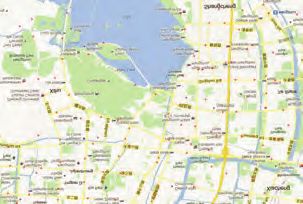
C2           C4              C2                                          Bus Stop Identification   Bus Route Selection
                                                              C4
          C1                           C1
                                                                                                 Hot Grid Cell           Graph Building
                         C3                           C3                                          Selection                & Pruning

                                  C7                          C7
               C5                           C5                                                   Merge & Split           Automatic Bus
                         C6                           C6
                                                                                                                        Route Generation

Fig. 1. An illustrative example of the taxi GPS trajectories (left) and the                      Stop Location
                                                                                                                            Bus Route
converted bus routing graph (right).                                                               Selection
                                                                                                                            Selection

                                                                                       Fig. 2.   The two-phase bus route planning framework.
distributed in the whole city, with some areas having more
PDRs than other areas, but there is no clear guideline about
where the bus stops should be put. Thus there needs a method                     Second, we develop a novel process with effective methods
to identify candidate bus stops from taxi passenger pick-                     to cluster “hot” areas with dense passenger pick-up/drop-off,
up/drop-off distributions.                                                    split big “hot” areas into walkable size ones and identify
   Second, to deliver the maximum number of passengers, the                   candidate bus stops. It is verified that the proposed method
best bus route should leave from the bus origin C1 , go through               outperforms the popular k-means method in terms of sound-
all the intermediate bus stops, and finally reach the destination             ness of selected bus stop location and evenness of selected bus
C7 . That is, the bus route would follow the sequence of bus                  stop distribution.
stops as C1 → C2 → C5 → C3 → C4 → C6 → C7 . However,                             Third, we derive several effective rules to build the di-
the problem for this route is that the whole trip would take a                rected bus routing graph where nodes and edges represent
very long time to complete, which is intolerable if the number                the candidate bus stops and valid connections among stops,
of candidate bus stops is big. Thus, a non-trivial trade-off has              respectively. To ensure the bus would reach destination in the
to be made between the number of passengers expected along                    end and reduce the computation complexity, we also develop
the route and the total time travelled.                                       an iterative process to remove invalid nodes and edges.
   Third, as there is no taxi passenger travelling from C4 to                    Finally, we propose two heuristic algorithms for automati-
C7 in Fig. 1 (left), if we design the bus route as C1 → C2 →                  cally generating valid bus routes. One is the probability based
C3 → C7 , then the significant passenger flow in paths C2 →                   spreading algorithm which randomly selects the next stop
C4 and C3 → C4 cannot be accommodated. Alternatively, by                      among the possible candidate stops in each step, giving the
including C4 in the planned bus route as C1 → C2 → C3 →                       candidate stop with high accumulated passenger flow a big
C4 → C7 , all the passenger flows in C2 → C4 , C3 → C4 ,                      probability for random selection; the other is the top-k spread-
C2 → C7 and C3 → C7 are accommodated with the cost of                         ing algorithm which selects k nodes with high accumulated
adding one more stop. Therefore, even the path C4 → C7 has                    passenger flows as candidate stops in each step. It is verified
no passenger flow, but adding it to the planned bus route would               that the probability based spreading algorithm outperforms the
lead to a better solution due to passenger flow accumulation                  top-k approach in the selection of best bus routes.
from all previous stops and paths.
   Finally, besides the passenger flow accumulation along the                                          II. R ELATED WORK
bus route, we also need to consider that the passenger flows are                 Here, we briefly review the related work which can be
usually different from time to time. For instance, the passenger              grouped into two categories. The first category is about making
flow during 23:00-24:00 might be very different from that                     use of taxi GPS traces for urban planning and traffic manage-
during 3:00-4:00. Thus we have to consider the passenger                      ment. The existing work includes automatic map construc-
flows accumulated and the total number of passengers in all                   tion [3], detecting hot spots and frequent travel patterns [8],
concerned timeslots while selecting the planned bus route.                    predicting road traffic conditions [4], informing land use and
   In this paper, we propose a two-phase approach to address                  function distribution [11], [13], uncovering inefficient road
the above-mentioned challenges. In the first phase, we identify               network connectivity [18], planning optimal driving route [14]
the candidate bus stops leveraging the taxi GPS data. In the                  and various applications such as next passenger finding [15],
second phase, with all the candidate bus stops identified and                 anomalous trajectory discovery [17]. Among the taxi GPS
the bus route OD designated, we develop effective rules and                   trace related papers, the work addressing “hotspots” and
heuristic algorithms to generate the bus route with maximum                   frequent travel OD patterns are relevant to our work for
number of passengers expected under the time constraints,                     identifying candidate bus stops and providing passenger flow
with the process shown in Fig. 2. In summary, the main                        data among potential bus stops, but there is no paper except
contributions of this paper include:                                          one [2] using those data for bus route planning. The main
   First, we propose a two-phase approach to tackle the night-                goal of [2] is to mine historic taxi GPS trips to suggest a
bus route design problem leveraging the taxi GPS data. To the                 flexible bus route. The work first clusters trips with similar
best of our knowledge, this is the first work on night bus route              starting time, duration, origin and destination; it then attempts
design using the taxi travel speed, time and PDRs information.                to identify the route that connects multiple dense taxi trip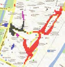
clusters. The work is different from ours as it only chooses the
route which maximizes the sum of each connected trip cluster.
In another word, it does not consider the time constraints and
the accumulated effects among connection stops, thus it would
never include the path like C4 → C7 of Fig. 1 in the planned
bus route, while our approach might include the path as long
as the route expects the maximum number of accumulated
passengers and the total travel time constraint can be met.
   The second category is about the bus network design,
which is an intensive studied area in urban planning and            Fig. 3. City partitions near Hangzhou Railway Station. Each city partition
transportation field. The bus network design is known to be         is marked with a different color.
a complex, non-linear, non-convex, multi-objective NP-hard
problem [10], [9]. The aim is to determine bus routes and
operation frequencies that achieve certain objectives, subject      cluster; (3) Choose one grid cell as the candidate bus stop
to the constraints and passenger flows. The popular objectives      location in each walkable size “hot” cluster, by assuming that
include shortest route, shortest travel time, lowest operation      passengers from the same cluster would easily walk to the stop
cost, maximum passenger flow, maximum area coverage and             to take the bus.
maximum service quality while the constraints include time,
                                                                    A. Hot Grid Cells and City Partitions
capacity and resources. However, the selection of the ob-
jectives should take care of the operator as well as user              In this work, we first divide the city into equal-sized grid
requirements which are often conflicting, leading to design         cells, with each cell about 10m × 10m. In such a way, the
trade-off rather than an optimal solution. As noted in [5],         whole city is partitioned into 5000 × 2500 cells in total.
early bus network design is mainly based on human survey            Out of all the grid cells, over 95% of them contain no taxi
to get passenger flows and user demands, it relies heavily on       passenger PDRs as they are either lakes, mountains, buildings,
heuristics and intuitive principles developed by a designer’s       and highways that cannot be reached or stopped by taxis, or
own experience and practice. Recent work on bus network             suburb areas that people seldom travel to. Only 0.11% of them
design also assumes that the passenger flows are given by user      have more than 0.2 PDRs per hour on average if we only count
survey or population estimation, the best solving algorithms        the PDRs in late night. And we name these grid cells as “hot”
are based on heuristic procedures to find sub-optimal solutions.    ones.
A detailed review about route network design can be found              As each grid cell has maximum eight neighbors, if we
in [7].                                                             define the connectivity degree (CD) of a “hot” grid cell as
   Despite the renewed attention for bus network design, there      the number of “hot” neighboring cells, the CD of any grid
is still no work addressing the night-bus route design problem      cell will range from 0 to 8, where the “hot” grid cell with
leveraging the taxi passenger OD flow data. Different from          CD equal to 0 is called isolated cell. As the city is composed
existing research, our work aims to find a bus route with a fixed   of mixed hot grid cells and common grid cells, both hot cells
frequency, maximizing the number of passengers expected             and common cells form irregular “hot areas” and “common
along the route subject to the total travel time constraint. This   areas” as a consequence of same type of cells being adjacent
problem is different from the traditional Travelling Salesman       to each other. These “hot areas” are also called city partitions,
Problem (TSP) [1] in nature, which aims to find the shortest        as shown in Fig.3. Apparently, some small partitions (like the
path that visits each given location (node) exactly once.           small ones in Fig. 3) can be very close to some big ones (like
TSP evaluates different routes with exact N locations, which        the black and red ones in Fig. 3). It would be necessary to
means all candidate stops should be included in the route.          consider all the city partitions globally in order to plan the
Our problem is also different from the shortest path finding        bus stop locations, thus city partitions close to each other had
problem [12], which intends to get the shortest path for a given    better merge to form big clusters for better overall bus stop
OD pair. In our case, we have to consider the accumulated           distribution. In the next section, we propose a simple strategy
effect (passenger flows) from all previous stops to current stop    to merge the close partitions into bigger clusters.
for choosing the bus route.
                                                                    B. Cluster Merging and Splitting
        III. C ANDIDATE B US S TOP I DENTIFICATION                    We present the cluster merging and splitting approach in
   In the proposed two-phase bus route planning framework,          Algorithm 1. After obtaining all city partitions, we sort them
the objective of phase one is to identify candidate bus stops       in a descending order according to the number of PDRs
by exploiting the taxi PDRs. The whole process consists of          (Line1). To merge the partitions close to each other iteratively,
three steps: (1) Divide the whole city into small equal-sized       we propose to use the hottest partition to absorb its nearby
grid cells, mark those “hot” grid cells with high taxi PDRs         partitions according to the descending order of PDRs, until
for further processing; (2) Merge the adjacent “hot” grid cells     no more nearby partitions meet the merging criteria (Line8).
to form “hot” areas, divide each big area into “walkable size”      Then we choose the next hottest partition to repeat the same
Algorithm 1 Merge Algorithm in horizonal and vertical directions, while for clusters in group
Input: List of partitions {Pi } 2, we only need to split the cluster in one direction. Fig. 4
Output: List of clusters {Ci }
1: P ← sort (P ), (i = 1, 2, · · · , n) // Sort P according to amount of its PDRs by shows an illustrative example of splitting a cluster into four
descending order sub-clusters with the proposed splitting strategy. The initial
2: i = 1;// Initialization
3: while P ̸= ∅ do cluster belongs to group 1 (Fig. 4 (left)), the splitting is first
4: Ci = {P1 }; done in horizontal direction to produce two sub-clusters with
5: P = P \{P1 } // Remove P1 from P
6: k = |P | ; similar PDRs. After the first splitting, two sub-clusters with
7: for j := 1 to k do width greater than 500m are generated, thus both sub-clusters
8: if dist(Ci , Pj ) < th (we set th to 150 m) then
9: Ci = Ci ∪ Pj //absorb the closer partition require a further splitting in vertical direction. The final result
10: P = P \{Pj } //Remove Pj from P with four split sub-clusters is shown in Fig. 4 (right).
11: end if
12: end for
13: i = i + 1; C. Candidate Bus Stop Location Selection
14: end while After merging and splitting operations, we obtain a big num-
ber of “hot” clusters with the size smaller than 500m × 500m.
The next step is to select a representative grid cell in each
cluster to serve as the candidate bus.
[ ]
CD(i) + 1 P DRs(i)
arg max w1 × + w2 × ∑n (2)
9 i=1 (P DRs(i))
To select this representative grid cell, both connectivity
degree (CD) and the number of PDRs of each cell in the
cluster are taken into consideration. While the CD of a grid
cell characterizes the accessibility of the cell, the number of
PDRs is an indicator of its “hotness”. The grid cell having the
Fig. 4. Illustrative example of splitting. Big cluster formed via merging (left).
Big cluster split into 4 walkable size clusters (right, in four different colors). maximum value defined in the Eq. 2 in each cluster is selected
as the “center” of the cluster, marked as the location of the
candidate bus stop. We set w1 = w2 = 0.5 in the evaluation,
process until all the partitions are checked (Line8∼Line12). and totally we get 579 candidate bus stops in the city.
The location of each partition is first initialized by computing IV. B US ROUTE S ELECTION
the weighted average location of all grid cells using the Eq. 1.
∑N After fixing the candidate bus stops in phase one, the aim
(P DRs(gi ) ∗ loc(gi )) of phase two is to find the best bus route for a given OD,
loc(P ) = i=1∑N (1)
expecting to maximize the expected number of passengers
i=1 P DRs(gi )
under the time constraints.
where loc(gi ) refers to the longitude/latitude of the member Here, we first approximate the passenger flow and travel
grid cell gi . time between any two candidate stops using taxi GPS traces,
After merging one partition, the location of the combined then we present the bus route selection method which contains
cluster is updated (Line9) and the absorbed partition is re- the following three-steps: 1) Build the bus routing graph and
moved from the partition list (Line 10). The dist function refers remove invalid nodes and edges iteratively based on certain
to the distance between two given partitions. The algorithm criteria; 2) Automatically generate candidate bus routes with
will be terminated until no partitions can be merged to a new two proposed heuristic algorithms; 3) Select the bus route by
cluster (Line3). comparing the expected number of passengers under the same
However, some merged clusters may be too large, which can total travel time constraint.
set up more than one bus stop. Thus proper splitting should
be done for these big clusters. In general, the merged clusters A. Passenger Flow and Travel Time Estimation
can be classified into three groups according to their size (the We record the travel demand and time information in two
size of cluster is defined as minimal rectangle which covers all matrix, named passenger flow matrix (FM) and bus travel
the grid cells): 1) with both height and width are greater than time matrix (TM). Each element in the matrix refers to the
500m; 2) with either height or width is greater than 500m; number of passengers and bus travel time from one stop (ith)
and 3) with both height and width are less than 500m. We to another stop (jth, i ̸= j). We count the total taxi trips from
find that only a very small number of clusters (around 10%, ith cluster to jth cluster as each stop is responsible for its
group 1 and 2) need further splitting operations. cluster. We set the maximum waiting time for passengers at
As for large clusters (group 1 and 2), we adopt a simple the stop is 30 minutes, so any pick-up or drop-off events taking
strategy to split them. Specifically, for clusters in group 1, we place in this time window are counted. We simply assume the
split the big cluster into a number of sub-clusters, aiming to passenger flows among candidate bus stops remain unchanged
minimize the difference of PDRs of the resulted clusters both during each 30-minutes duration. The final FM is got byY
averaging all flow matrix at different bus frequencies. We also
Ynew
assume TM keeps unchanged across the night time. tm(si , sj )
is the average travel time multiply by α, which is a constant. 1
2
We set α = 1.5 to consider the speed difference between 1
O
3
taxis and bus. For the paths having no taxi trip occurring in O
X
history (for instance, nobody travels by taxi due to too short θ
2
D
distance), we use Ddist(si ,sj )/v to approximate tm(si , sj ), 3 Xnew D 4
where Ddist(si , sj ) is the driving distance between si and sj ,
and v is set to 50 km/h. Fig. 5. Demonstration of Criteria 2 (left) and Criteria 5 (right).
B. Bus Routing Graph Building and Pruning
Selecting the best bus route is a very challenging problem value of X-axis of stop in the new coordination which is
as two conflicting requirements must be met: one is to ensure with s1 as the origin, and from s1 to sn as the direction
that the bus route would traverse intermediate stops and finally of X-axis (see the left panel in Fig. 5). This criteria
reach the destination within a limited time; the other is to guarantees the bus will always move forward along the
maximize the number of passengers accumulated along the OD direction.
route. For example, if we choose the stop with the heaviest • Criteria 3: Source-farther
passenger flow from the origin as the first node, and then
keep choosing the next stop following the heaviest passenger dist(si+1 , s1 ) > dist(si , s1 ) (i = 1, 2, · · · , n − 1)
flow principle, then we might neither reach the destination, This ensures that the bus will move away from the origin
nor achieve the objective of having the maximum number of s1 farther in each step.
passengers accumulated along the route. To meet the above • Criteria 4: Destination-closer
two requirements and follow the intuitive principles in bus
route design, some basic criterion should be set for bus routing dist(si+1 , sn ) < dist(si , sn ) (i = 1, 2, · · · , n − 1)
graph building and candidate bus route selection.
1) Routing graph building criteria: Obviously, there would This ensures the bus will move closer to the destination
be numerous stop combinations for a given OD pair, and only a sn in each step.
small proportion of them meet the first or second requirement. • Criteria 5: No zigzag route
To reduce the search space of possible stops and routes, we can arg min(dist(si+1 , sj )) = si (j = 1, 2, · · · , i)
build a bus routing graph starting from origin to destination | {z }
sj
using heuristic rules. For instance, from the shortest travel time
perspective, the bus route should extend from origin towards Criteria 5 ensures the smoothness of the route. There
the direction of destination, it can be further converted into would be no sharp zigzag path along the OD direction.
three rules: each new selected stop should be farther from The route demonstrated in the right panel of Fig. 5 should
the origin, closer to destination, and farther from previous not happen, as it violates the no zigzag route criteria. We
stop. From the intuitive bus route design principle, the bus can see arg min(dist(s3 , sj )) = s1 ̸= s2 (j = 1, 2), also
stops should not be too far from each other, also the bus route arg min(dist(s4 , sj )) = s2 ̸= s3 (j = 1, 2, 3).
should not comprise sharp zig-zag paths. These can also be 2) Graph building and pruning: The aim of graph building
translated into two criterion in building the bus routing graph. is to construct a directed graph with nodes and links given an
Specifically, given the OD pair (s1 , sn ) and the candidate route OD pair, in which the nodes are the stops, and edges link the
R = ⟨s1 , s2 , · · · , sn ⟩, we should obey the following criterion stop to its next possible stops, regardless of passenger flows
when building the bus routing graph. among them. While the goal of graph pruning is to remove
• Criteria 1: Adequate stop distance invalid edges and nodes according to the proposed criterion.
dist(si+1 , si ) < δ (i = 1, 2, · · · , n − 1) Graph Building: Given the bus route OD, their locations
are firstly used to narrow down the choice of valid candidate
where δ is a user-specified parameter. We set δ = 1.5 km, stops, only the candidate stops lying between them are under
which means the maximum distance between two consec- consideration. For each stop within the range, we determine
utive stops should be no more than 1.5 km. links to its next possible stops according to the proposed
• Criteria 2: Move forward Criteria 1∼4. As Criteria 5 is related to all stops in one bus
xnew (i + 1) > xnew (i) (i = 1, 2, · · · , n − 1) route, so we use it to prune the routing graph after it is built.
xnew (i) = x(i) cos θ + y(i) sin θ Fig. 6 (left) shows an illustrated example about a generated
bus routing directed graph.
y(n)
θ = tan−1 Graph Pruning: Some nodes and edges can be further
x(n) pruned because they are not useful for valid candidate bus
(x(i), y(i)) of the si is got by simply subtracting the route selection. To be specific, for nodes without in-coming
longitude and latitude value to that of s1 . xnew is the edges (if not origin) or out-going edges (if not destination),Algorithm 2 Probability based Spreading
O O
Input: G(S, E); flow Matrix
Output: R∗
1: R = ∅
2: Repeat
3: currentR = s1
D D 4: Choose the next stop s∗i with respect to currentR according to Eq. 5
5: R = currentR·s∗i
//· operation appends si to currentR
6: Repeat Lines 4∼5 Until s∗i = sn
Fig. 6. A bus routing directed graph for a given OD. 7: R = R ∪ R
8: Get corresponding skyline routes R∗
9: Until R∗ keeps unchanged
as they will not form any valid routes with the bus route OD
pair, these edges and nodes should be deleted.
We first calculate all the nodes’ in-coming and out-going route is chosen based on Eq. 5.
∑j
degrees. And nodes (exclude the given OD) and corresponding f m(sm , s∗i )
edges would be iteratively deleted from graph if their in- P (s∗i |⟨s1 , s2 , · · · , sj ⟩) = ∑|S ∗ |m=1
∑j (5)
∗
i=1 m=1 f m(sm , si )
coming or out-going degree is zero. At last graph with only
one zero in-coming degree (given origin) and one zero out- where f m(sm , s∗i ) is the passenger flow from sm to s∗i , and
going degree (given destination) would be generated. After S ∗ contains the next possible stops of sj (child nodes of sj
graph pruning, all the bus routes starting from the source in routing graph).
and following the edges in the graph would eventually reach We can see the selection of next stop in the candidate route
the destination. Fig. 6 (right) displays the resulted graph after is not only determined by the current stop, but also all the
applying pruning to the graph in Fig. 6 (left). previous stops. The output of this algorithm is one candidate
bus route with the number of stops associated with the number
C. Automatic Candidate Bus Route Generation of spreading steps. The spreading would be terminated when
Probability based Spreading Algorithm: Though we have the given destination is reached (Line6). For each run, we get
removed invalid nodes and edges through graph pruning, the either a repeated route or new route, thus the candidate route
problem of enumerating all possible routes from given source set R would increase as the spreading algorithm is activated.
to destination is proved to be NP hard. Indeed, it is also Then a question arises: how many times are sufficient to run
unnecessary to enumerate all possible routes and compare the spreading algorithm and get the best results ? Based on
them all, because most of routes are dominated by few others. Definition 1 about the skyline routes, we should consider if
the skyline route set R∗ remains changed or unchanged.
D EFINITION 1. We say Ri dominates Rj iif: 1) T (Ri ) ≤
Theorem 1 below ensures that when the skyline route set
T (Rj ); 2) N um(Ri ) > N um(Rj ).
stays unchanged with the increase of spreading algorithm runs,
where T and N um are the total travel time and number of
then the best route has been discovered.
expected delivered passengers, which is computed based on
Eq. 3 and 4. Theorem 1. R∗1 and R∗2 are the detected skyline routes from
R1 and R2 respectively. If R1 ⊆ R2 , then we have: ∀Ri ∈
∑
n−1
T = tm(si+1 , si ) + (n − 2) × t0 (3) R∗1 , ∃Rj ∈ R∗2 ; Ri = Rj or Ri is dominated by Rj .
i=1 In Algorithm 2, we have Rt1 ⊆ Rt2 if the running time
∑
n t1 < t2 , and the algorithm would be stopped when no better
N um = f m(si , sj ) (4) skyline routes are returned with the increase of running times,
i;j(j>i) that is R∗t1 = R∗t2 (Line9). Instead of choosing only one
stop randomly at each spreading step like in the probability
where t0 is the bus waiting time at each stop, and we set based spreading algorithm, an intuitive way is to select top-
it to 1.5 minutes. The definition is similar to the skyline k stops each time, where those k nodes should have highest
routes in [6], and the rational behind is that only routes with accumulated passenger flow with previous stops; In such a
less travel time but larger number of passengers should be way, the first step selects top-k nodes, thus leading to k
selected. Skyline detector [18] will prune the routes which are routes from the origin to those nodes; In the second step,
dominated by skyline routes in the candidate set. Thus, the each k nodes would select another top-k nodes, thus the
comparison can be done among detected skyline routes. total candidate routes would be k 2 ; Assume reaching the
The key idea of our proposed probability based spreading destination needs n step spreading, then the total candidate
algorithm is to randomly select the next stop among the routes generated would be k n in the end. We use this top-k
possible candidate stops in each step, where the candidate spreading method as the baseline.
stops having high accumulated passenger flow with previous
stops are given high probability for random selection. We D. Bus Route Selection
describe the approach in Algorithm 2. The spreading starts Given the bus operation frequency (once every 30 minutes)
from the given source (Line3). The next stop in the candidate and the taxi passenger flow from 21:30 to 5:30, we obtain the1 1600
1400
0.8
(s) (s)
OD Pair 1 1200
Similarity
Cost
OD Pair 2 1000
0.6
Similarity
Time Cost
800
OD Pair 3
Time
0.4 600
400
0.2
200
0 0
0 1 2 3 4 5 6 7 8 9 10 11 12 13 14 15
Number of Running Times 4
Number of Runs x 10
Fig. 7. Comparison results with k-means. Results got by k-means (left) and
results got by our method (right). Fig. 8. Convergence study of the proposed spreading algorithm.
TABLE I
D ETAILED INFORMATION ABOUT STUDIED OD PAIRS
candidate bus routes for a given OD pair and maximum travel
time using the two different heuristic spreading algorithms, the OD Pairs Distance (km) Number of Stops
skyline route which achieves the maximum expected number
1 ZJU - Railway 5.70 104
of passengers will be selected as the operating route. With the 2 Railway - East Railway 5.86 75
planned bus route consisting of the selected bus stops, the next 3 East Railway - ZJU 8.80 144
step is to find a physical bus route in the real setting, which
consists of road segments. The selection of each road segment
is done by following the dense and fine trajectories of taxis if baseline approach. Table I shows the details of three OD pairs
they allow buses to operate; Otherwise similar bus routes near for night-bus route design experiment, where more than 70
the planned ones can be adopted as a refined solution. candidate bus stops are in the candidate bus route selection
list.
V. E XPERIMENTAL E VALUATION 1) Convergence Study: As illustrated in Algorithm 2, our
Here, we validate the proposed approach with a large-scale proposed bus route generation process would be terminated
real-world taxi GPS dataset which was generated from 7,600 if the resulted skyline routes keep unchanged. We study the
taxis in a large city in China (Hangzhou) for one month, with similarity of consecutively generated skyline routes from 5,000
more than 1.57 million of night passenger-delivering trips. to 150,000 runs, with a constant interval of 5,000 runs. We
measure the similarity (sim) of two sets A and B as follows:
A. The Identification of Candidate Bus Stops
|A ∩ B|
We compare the bus stop results generated with our method sim(A, B) = (6)
|A ∪ B|
with that generated by the popular k-means clustering method.
We set k = 579, which is the same as our method. We adopt The similarity results of the consecutively generated skyline
the Eulerian distance as the similarity metric. The centroid of routes with a 5,000 run interval are shown in Fig. 8, the
each cluster is selected as the stop. Fig. 7 shows the compar- time cost is put in the diagram as well. In this study, we
ison results. Comparing with the popular k-means approach, can see sim values gradually reach 1 with the increase of
our proposed candidate bus stop identification method has two runs for all three OD pairs, meaning that in all three cases
advantages: 1) the centroid of each cluster got by k-means is the best bus route converges to one. Also the time cost is
the average location of all its members, and it may fall into almost linearly increased with the number of runs, suggesting
non-reachable places like river, as highlighted by the green that the spreading time cost at each run is almost constant.
circle in Fig. 7 (left). In our proposed method, both hotness It is also noted that the three curves for three OD pairs have
and connectivity of each grid cell is considered for bus stop different slopes, the reason is probably because the bus routes
location selection, and the selected bus stops are meaningful corresponding to different ODs have different lengths and
and stoppable places; 2) Several identified stops by k-means varied number of candidate bus stops, thus the spreading time
fall into a small area (highlighted by the blue circles) as and candidate bus stop selection time should be also different.
the size of clusters got by k-means is very different, while 2) Candidate Routes Statistics: Fig. 9 shows the statistical
our proposed method generates candidate bus stops that are information about the number of stops of candidate routes.
evenly distributed in the hot areas, which meets better the Several interesting observations can be made:
commonsense design criteria of bus stops. • For OD pair 1, routes with 8∼10 stops take up over 80%
of the cases (both origin and destination are included).
B. Evaluation of the Probability based Spreading Algorithm Few routes can reach the destination by traversing only
We evaluate our probability based spreading approach. We 4 stops, or passing more than 11 stops.
first show the convergence of the proposed algorithm. Then we • For OD pair 2, over 60% of the routes contain 9 or 10
perform a quantitative statistical analysis of all the candidate stops. Similar to the case of OD pair 1, some routes can
routes generated for three given OD pairs. We will also give reach the destination by passing 4 stops.
the computed skyline route results. Finally, we validate that • For OD pair 3, most of the routes contain 10 to 18 stops
our proposed bus route generation approach outperforms the due to the longer OD distance, and almost half of the40 25
of Passengers
35 OD Pair 1
Number of Delivered Passengers
OD Pair 2 20
Percentages(%) (%)
30
OD Pair 3
Percentages
25
15
20
k=2
15 10 k=3
Number
k=4
10 k=5
Random
5
5
0
4 5 6 7 8 9 10 11 12 13 14 15 16 17 18 19 20 21 22
Number of Stops 0
Number of Stops 1000 2000 3000 4000 5000 6000 7000
Total Travel Time (s)
8000 9000 10000
Total Travel Time (s)
Fig. 9. Statistical information about candidate route stops for 3 OD pairs.
Fig. 11. Comparison results with baseline under different k values.
1818
Number of Passengers
1616
1414
access all the taxi passenger flows before the route started
Number of Delivered Passengers
1212
1010
88
date. It is noted that the route is designed by local experts and
66 the user demands are obtained from expensive human survey.
44
We first draw the newly started night-bus route on Google
22
01000
0
1000 2000
2000
3000
3000
4000
4000
Total5000
Travel Time (s)6000
5000 6000
7000
7000
8000
8000
9000
9000
map as shown in Fig. 12 (left bottom), then we draw our
Total Travel Time (s) proposed night-bus route R1 in Fig. 12 (left top). Through
comparison we see that they are quite different. With the newly
Fig. 10. Detected skyline routes and other candidate routes.
started route, we decide to take a similar route in our selected
candidate bus routes (not the best one), and we find R2 as
routes include 13 or 14 stops. shown in Fig. 12 (left top). It is noted that the main difference
• The statistical results comply with the intuition that the between R2 and the newly started route is that R2 includes
longer distance of a given OD pair, the more stops the an additional Stop J in the route. By comparing the passenger
route would contain. flow in segment I→K with that in segment J→K at different
time slots, it is found that the passenger flow in path J→K is
3) Skyline Routes: We show the skyline routes for the OD
even greater than I→K in the first two time slots, as shown
pair 2 in Fig. 10. Each point in the plane represents a candidate
in Fig. 12 (right top). Considering further the accumulation
route. The x-axis stands for the total travel time of candidate
effects, including Stop J in the bus route would significantly
route, while the y-axis represents the expected number of
increase the expected number of passengers along the route.
passengers. From Fig. 10, we can see that the skyline routes
Thus, our candidate bus route R2 would outperform the newly
are connected to form a curve above all the points representing
added bus route, at the cost of adding one more bus stop and
common routes, and over 99% of the routes are dominated by
more travel time.
the few skyline routes. Specifically, we get 40 skyline routes
We also compare our proposed best route R1 with the
across all the travel time frames, out of hundreds of thousands
candidate route R2 . The difference between R1 and R2
of routes for the case of OD pair 2. Similar phenomena have
lies in two different paths taken from C to H. While R2
been observed for other two cases as well.
passes the famous shopping street (Yan’an Road) in Hangzhou
4) Comparison with top-k spreading algorithm: In top-k
(C → E → F → H), R1 traverses the famous night-club
spreading algorithm, the selection of k is vital to the skyline
areas along the West Lake. If we compare the number of
routes generated as well as the time needed to generate all
passengers in R1 and R2 , it can be seen from Fig. 12 (right
the candidate routes. In particular, when k1 < k2 , we have
bottom) that the passenger flow of R2 is heavier than that of
Rk1 ⊆ Rk2 (k1 ≤ k2 ). Theorem 1 guarantees that a bigger
R1 only around 22:00, and it is much lighter soon after 23:00.
k would lead to a better set of skyline routes. However, the
With the rest of the stops being the same for both R1 and R2 ,
greater k also results in significantly increase of time cost.
there is no doubt about why R1 has been selected as the best
We compare the skyline routes generated from the probability
night-bus route. If we take a closer look at R1 , R2 , and the
based spreading method with that from the top-k spreading
newly started route, as R1 takes a much shorter route than
method with different k value, which is shown in Fig. 11.
R2 and needs similar travel time as the newly started route
We can see that the probability based spreading approach
does, but R1 expects much more passengers than R2 and the
outperforms the top-k algorithms even when k is set to 5.
newly started route, thus it is reasonable to conclude that the
C. Comparison with Real Routes selected night-bus route with our proposed approach is better
As the taxi GPS dataset we have was collected from April than the current route-in-service in terms of travel time as well
2009 to March 2010, we are very interested in knowing if there as expected number of passengers.
was any new night-bus route created during this year and how
VI. C ONCLUSION AND F UTURE W ORK
the planned bus route generated with our approach compares
with the manually created route. Fortunately we were told that In this paper, we have investigated the problem of night-
a night-bus route was created in February 2010, we could bus route design by leveraging the taxi GPS traces, whichE 4.5
B
C
F 4 J→ K limitation; 3) Currently we only explore the issue of designing
Passenger FlowFlow
3.5
A 3
I→ K
the best bus route for a given OD pair, the proposed approach
Passenger
D
G
H
2.5
2
is still unable to tackle the design of a bus route network.
I
1.5 In the future, we plan to broaden and deepen this work in
1
K
0.5 several directions. First, we attempt to investigate the optimal
J
0
2 4 6 8 10
BusBusFrequency
12
Frequency
14 16 bus route design with more real-life assumptions such as varied
30 bus operation frequency and limited bus capacity; Second, we
Passengers
R1
25
plan to study the impact of parameter change on the bus route
of Passengers
R2
20
design and the added bus route on the taxi services along the
15
Number of
bus route; Third, we would like to develop practical systems
Number
10
5
leveraging on taxi GPS traces, enabling a series of pervasive
0
2 4 6 8 10 12 14 16
smart transportation services.
Bus Frequency
Bus Frequency
ACKNOWLEDGEMENTS
Fig. 12. Results comparison. Planned routes (top left); Passenger flow We would like to thank the shepherd, Dr. Petteri Nurmi,
comparison of two segments at different frequency (top right); Opened night-
bus routes (bottom left); Number of delivered passengers at different frequency
and the reviewers for their constructive suggestions. This
(R1 vs R2 , bottom right). research was partially supported by the Paris-Region SYS-
TEM@TIC Smart City “AQUEDUC” Program, NSF of China
(No. 61105043), and JiangsuSF (BK2011566).
is motivated by the needs of applying pervasive sensing, R EFERENCES
communication and computing technology for sustainable city [1] D. L. Applegate, R. E. Bixby, V. Chvatal, and W. J. Cook. The Traveling
development. To solve the problem, we propose a two-phase Salesman Problem: A Computational Study. Princeton University Press,
approach for night-bus route planning. In the first phase, we 2007.
[2] F. Bastani, Y. Huang, X. Xie, and J. W. Powell. A greener transportation
devise method to identify locations of the candidate bus stops, mode: flexible routes discovery from GPS trajectory data. In Proc. of
with the passenger pick-ups and drop-offs as inputs. In the GIS, pages 405–408, 2011.
second phase, with the bus route origin, destination, and can- [3] L. Cao and J. Krumm. From GPS traces to a routable road map. In
Proc. of the ACM GIS, pages 3–12, 2009.
didate bus stops as inputs, we develop two heuristic algorithms [4] P. S. Castro, D. Zhang, and S. Li. Urban traffic modelling and prediction
to automatically generate candidate bus routes, and finally we using large scale taxi GPS traces. In Proc. of Pervasive Computing,
select the best route which expects the maximum number of pages 57–72, 2012.
[5] T. A. Chua. The planning of urban bus routes and frequencies: A survey.
passengers under the given conditions. On a real-world dataset Transportation, 12(2):147–172, 1984.
which contains more than 1.57 million passenger delivery [6] Y. Ge, H. Xiong, A. Tuzhilin, K. Xiao, M. Gruteser, and M. Pazzani.
trips, we compare our proposed candidate bus stop identifi- An energy-efficient mobile recommender system. In Proc. of ACM
SIGKDD, pages 899–908, 2010.
cation method with the popular k-means clustering method [7] V. Guihaire and J.-K. Hao. Transit network design and scheduling: A
and show that our method can generate more reasonable global review. Transportation Research Part A: Policy and Practice,
and meaningful results. We further extensively evaluate our 42(10):1251 – 1273, 2008.
[8] L. Liu, C. Andris, and C. Ratti. Uncovering cabdrivers’ behavior patterns
proposed probability based spreading algorithm for automatic from their digital traces. Computers, Environment and Urban Systems,
bus route generation and validate its effectiveness as well as 34(6):541 – 548, 2010.
its superior performance over the heuristic top-k spreading [9] B. M.H. and M. H.S. TRUST: A Lisp program for the analysis of transit
route configurations. Transportation Research Record, 1283:125–135,
algorithm. Further more, we show the selected night-bus route 1990.
with our proposed approach is better than a newly started [10] G. F. Newell. Some issues relating to the optimal design of bus routes.
night-bus route-in-service in Hangzhou, China. Transportation Science, 13(1):20–35, 1979.
[11] G. Pan, G. Qi, Z. Wu, D. Zhang, and S. Li. Land-use classification
This work is among our initial attempts to apply pervasive using taxi GPS traces. IEEE Trans. on ITS, (99):1–11, 2012.
computing techniques in achieving better urban planning of [12] Z. Wang and J. Crowcroft. Analysis of shortest-path routing algorithms
smart cities. With the constraints of the approach and the in a dynamic network environment. SIGCOMM Comput. Commun. Rev.,
22(2):63–71, 1992.
acquired data, this work still has several limitations: 1) Human [13] J. Yuan, Y. Zheng, and X. Xie. Discovering regions of different functions
mobility patterns uncovered by taxi GPS traces are biased in a city using human mobility and POIs. In Proc. of ACM SIGKDD,
and incomplete, thus the designed bus route might not be the pages 186–194, 2012.
[14] J. Yuan, Y. Zheng, C. Zhang, W. Xie, X. Xie, G. Sun, and Y. Huang.
best, considering the fact that taxi traffic does not reflect the T-drive: driving directions based on taxi trajectories. In Proc. of the
whole passenger flow and people taking taxis might not be GIS, pages 99–108, 2010.
willing to switch to public transport for various reasons; 2) [15] J. Yuan, Y. Zheng, L. Zhang, X. Xie, and G. Sun. Where to find my
next passenger. In Proc. of UbiComp, pages 109–118, 2011.
The work makes some assumptions in problem formulation [16] D. Zhang, B. Guo, and Z. Yu. The emergence of social and community
and evaluation, for example, for bus stop determination we intelligence. Computer, 44(7):21 –28, 2011.
set the walkable distance as 500 meters and the threshold for [17] D. Zhang, N. Li, Z.-H. Zhou, C. Chen, L. Sun, and S. Li. iBAT: detecting
anomalous taxi trajectories from GPS traces. In Proc. of UbiComp, pages
cluster split and merge is 150 meters, apparently the choice 99–108, 2011.
of those parameters would affect the results, but a study of [18] Y. Zheng, Y. Liu, J. Yuan, and X. Xie. Urban computing with taxicabs.
the parameter sensitivity is not provided due to the space In Proc. of UbiComp, pages 89–98, 2011.You can also read