Equilibrium Module - Description of Menus and Options - Metso Outotec
←
→
Page content transcription
If your browser does not render page correctly, please read the page content below
HSC – Equilibrium Module
                                                                                               1/57
                                                                                               Petri Kobylin, Lena Furta, Danil Vilaev

                                                                                               December 11, 2020

13.            Equilibrium Module - Description of
               Menus and Options

Metso Outotec reserves the right to modify these specifications at any time without prior notice. Copyright © 2021, Metso Outotec Finland Oy
HSC – Equilibrium Module
                                                                                               2/57
                                                                                               Petri Kobylin, Lena Furta, Danil Vilaev

                                                                                               December 11, 2020

               SUMMARY

               HSC Equilibrium module enables user to calculate multi-component equilibrium
               compositions in heterogeneous systems easily. The user simply needs to specify the
               chemical reaction system, with its phases and species, and give the amounts of raw
               materials. The program calculates the amounts of products at equilibrium in isothermal
               and isobaric conditions.

               The user must specify the substances and potentially stable phases to be taken into
               account in the calculations as well as the amounts and temperatures of raw materials.
               Please note that if a stable substance or phase is missing in the system definition, the
               results will be incorrect. The specification can easily be made in the HSC program
               interface.

               The equilibrium composition is calculated using the GIBBS solver, which uses the
               Gibbs energy minimization method1. The program reads the result files and draws
               pictures and tables of the equilibrium configurations if several equilibria have been
               calculated. The user can toggle between the equilibrium and graphics programs by
               pressing the buttons.

               This version of the Equilibrium module also includes support for electrochemical
               calculations (previously known as Cell module). In Cell Equilibrium calculations, user
               also needs to specify the electrode phases, types of phases (gas/liquid/solid/metal),
               capacitances and discharge equation for the charging/discharging reaction.

               The main format Equilibrium module is *.gem9, which contains all the data and
               formatting settings of each definition sheet as well as the phase names. The program
               can also read imported files from the previous HSC versions:

               *.GEM file format contains all the data and formatting settings of each definition sheet
               as well as the phase names, etc. while the *.IGI file format contains the data for
               calculations only. *.ICE file format contains the data for single-point calculations of Cell
               Equilibrium.

Metso Outotec reserves the right to modify these specifications at any time without prior notice. Copyright © 2021, Metso Outotec Finland Oy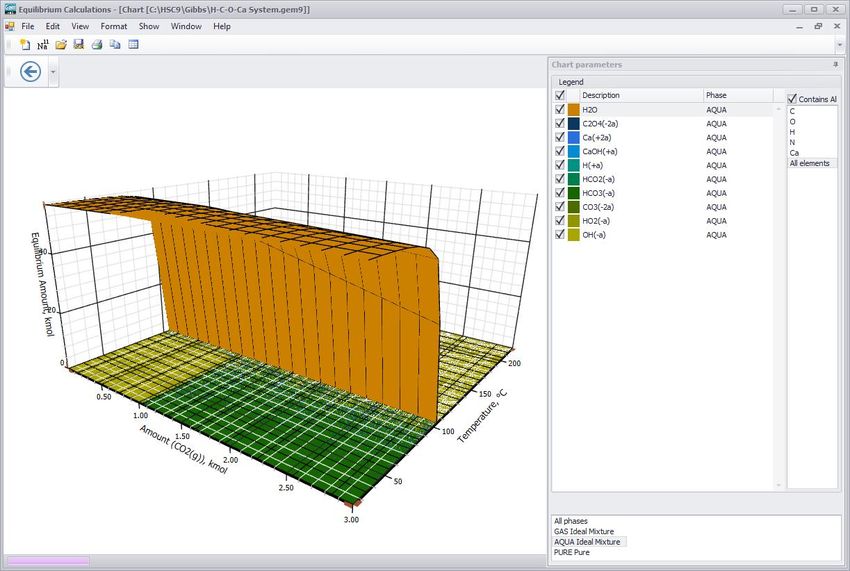
HSC – Equilibrium Module
                                                                                               3/57
                                                                                               Petri Kobylin, Lena Furta, Danil Vilaev

                                                                                               December 11, 2020

13.1.          Starting the HSC Equilibrium Module

               Fig. 1. Starting screen.

               There are three ways of creating an input file, see Fig. 1.

               1.      Press From Elements. Then specify the elements which are present in users
                       system, see Fig. 3. The HSC program will search for all the available species in
                       the database and divide them, as default, into gas, condensed and aqueous
                       phases. The user can then edit this preliminary input table.
               2.      Press Empty file if user is already certain of the possible substances and phases
                       of the system.
               3.      Press Open if user already has an input file which can be used as a starting file.
                       Edit the input table and save it using a different name.

Metso Outotec reserves the right to modify these specifications at any time without prior notice. Copyright © 2021, Metso Outotec Finland Oy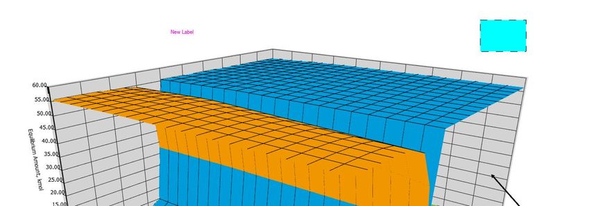
HSC – Equilibrium Module
                                                                                               4/57
                                                                                               Petri Kobylin, Lena Furta, Danil Vilaev

                                                                                               December 11, 2020

               If user has an old file format (*.GEM or *.IGI) user can import it from the File menu by selecting
               Import and working with it. User can update thermodynamic data of the file to HSC database
               values by Update species data from Edit menu, see Fig. 2.
               .

               If user only wants to calculate the equilibrium compositions and draw a picture with the
               existing files, press Calculate and then press Show Chart.

               Fig. 2. Update species data of the old file.

Metso Outotec reserves the right to modify these specifications at any time without prior notice. Copyright © 2021, Metso Outotec Finland Oy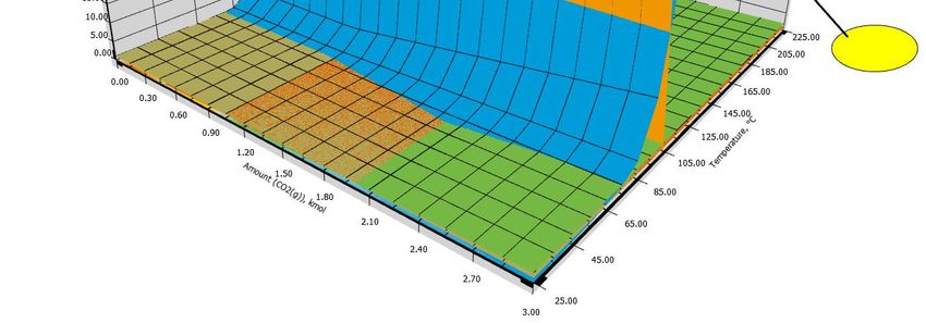
HSC – Equilibrium Module
                                                                                               5/57
                                                                                               Petri Kobylin, Lena Furta, Danil Vilaev

                                                                                               December 11, 2020

13.2.          Starting by Defining the Elements

               Fig. 3. Specifying the elements of the chemical system.

               Choose element from periodic chart or type them to first text filter. If user wants to
               choose only some of the species in the list in calculations, then select them (with ctrl
               button) and right-click and Import to Selected Species, see Fig. 4.

               By decreasing the number of species, user can increase the calculation speed and
               make the solution easier. Especially if user has selected C and/or H among the other
               elements, a very large number of species will be included in the calculation and user is
               advised to decrease the number of species. User can of course try with all the species,
               but usually it is wise to select only such species to the system which may be stable.

               However, if the stable species are not chosen, the calculated equilibrium results will be
               incorrect.

               If there is an odd species in the list then user can click the relevant formula in the list
               which will reveal the whole data set of the species in the database, see Fig. 4.

               The species have been divided into rough reliability classes in the database.

Metso Outotec reserves the right to modify these specifications at any time without prior notice. Copyright © 2021, Metso Outotec Finland Oy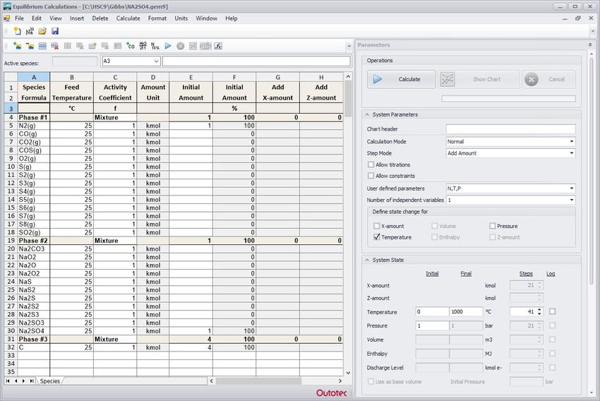
HSC – Equilibrium Module
                                                                                               6/57
                                                                                               Petri Kobylin, Lena Furta, Danil Vilaev

                                                                                               December 11, 2020

               Fig. 4. Choosing desired species to calculation.

               Press Import Species and user can also set the sorting order for the species. User
               can select one of the following sorting methods: Phases (species will be sorted by
               classes), Gas, Aqua, Pure (this sorting method is used for low temperatures), No
               sorting (all species will be in one phase) and Gas, Aqua, Liquids (melt will be added
               to individual class). The sorting order will determine the order of species in the
               Equilibrium Editor, see Fig. 5.

               When user has chosed sorting order of species, press OK and user will return to the
               Equilibrium Editor window, see Fig. 5.

Metso Outotec reserves the right to modify these specifications at any time without prior notice. Copyright © 2021, Metso Outotec Finland Oy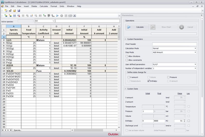
HSC – Equilibrium Module
                                                                                               7/57
                                                                                               Petri Kobylin, Lena Furta, Danil Vilaev

                                                                                               December 11, 2020

13.3.          Giving Input Data for Equilibrium Calculations

               Fig. 5. Specification of the species and phases for the reaction system. User can change
               solution model from Species sheet phase row (Column C).

               The calculation data is specified using the Parameters panel, Fig. 6. User gives all the
               data required to create an input file for the equilibrium solvers and for calculating the
               equilibrium compositions in the Species and Parameters panel sheets, see Fig. 5 and
               Fig. 6.

               The most demanding step is the selection of the species and phases, i.e. the
               definition of the chemical system. This is done in the Species sheet of the
               Equilibrium Editor, Fig. 5. User can move around the table using the mouse, or Tab
               and Arrow keys. The other points user should consider are:

               1. Species (substances, elements, ions...)

Metso Outotec reserves the right to modify these specifications at any time without prior notice. Copyright © 2021, Metso Outotec Finland Oy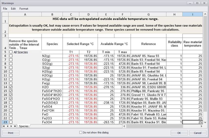
HSC – Equilibrium Module
                                                                                               8/57
                                                                                               Petri Kobylin, Lena Furta, Danil Vilaev

                                                                                               December 11, 2020

               User can type the names of the species directly into the Species column, without a
               preliminary search in the Elements window. If user has made the search on the basis
               of the elements, user will already have the species in the Species column.

               User can insert an empty row in the table by selecting Row from the Insert menu or by
               pressing the right mouse button and selecting Insert Row from the pop-up menu.

               Rows can be deleted by selecting Row from the Delete menu or by pressing the right
               mouse button and then selecting Delete Row from the pop-up menu.

               User can change the order of the substances by inserting an empty row and using the
               copy - paste method to insert a substance in a new row.

               Use the (l)-suffix for a species only if user wants to use the data of liquid phases at
               temperatures below their melting point. For example, type SiO2(l) if SiO2 is present in a
               liquid oxide phase at temperatures below the melting point of pure SiO2. User may also
               use (s)-suffix if user wants to force Gibbs to use solid data at any temperature.

               The species can be inserted by selection Species in the Insert menu. Then the
               Browse Database window will appear where user will find the species that user needs.
               User can use search, or type a formula or chemical name in the search string, and the
               program will find the species.

               User can also type a species formula in a new row in the Equilibrium Editor window,
               and the program will suggest species if predictive typing is selected in the Edit menu.

               2. Phases

               The species selected in the previous step must be divided into physically meaningful
               phases as determined by the phase rows. This finally defines the chemical reaction
               system for the equilibrium calculation routines. The definition of the phases is
               necessary because the behavior of a substance in a mixture phase is different from
               that in pure form. For example, if we have one mole of pure magnesium at 1000 °C, its
               vapor pressure is 0.45 bar. However, the magnesium vapor pressure is much smaller if
               the same amount has been dissolved into another metal.

               The phase rows must be inserted in the sheet using the Phase selection in the Insert
               menu or using the same selection in the pop-up menu of the right mouse button. The
               Equilibrium module makes the following modifications to the sheet automatically when
               user inserts a new phase row in the sheet and:

               1.      Requests a name for the new phase, which user can change later, if necessary.
               2.      Inserts a new empty row above the selected cell of the sheet with a beige pattern.
               3.      Assumes that all rows under the new row will belong to the new phase down to
                       the next phase row.
               4.      Inserts new Excel-type SUM formulae in the new phase row. These formulae
                       calculate the total species amount in the phase using kmol, kg, or Nm3 units.

               When the insert procedure is ready, user may edit the phase row in the following way:

               1.      The phase name can be edited directly in the cell.

Metso Outotec reserves the right to modify these specifications at any time without prior notice. Copyright © 2021, Metso Outotec Finland Oy
HSC – Equilibrium Module
                                                                                               9/57
                                                                                               Petri Kobylin, Lena Furta, Danil Vilaev

                                                                                               December 11, 2020

               2.      The phase temperature can also be changed directly in the cell and will change
                       the temperatures of all the species within the phase. Note that phase and species
                       temperatures have effect only on the reaction enthalpy balances. Equilibrium
                       temperatures must be specified in the Parameters panel, see Fig. 6.
               3.      Note also that user cannot type formulas in the amount column of the phase row,
                       because the SUM formulas are located there. User can change the unit used
                       from the Units menu.

               The first phase to be defined is always the gas phase, and all gaseous species must be
               under the gas phase row. Species of the same phase must be given consecutively one
               after another in the table. As default, HSC Chemistry automatically relocates all the
               gaseous species, condensed oxides, metals, aqueous species, etc. into their own
               phases if user starts from the “give Elements” option, see Fig. 1. The final allocation,
               however, must be done by the user.

               If there is no aqueous phase, all aqueous species must be deleted. Note that if user
               has an aqueous phase with aqueous ions, user must also have water in the phase!

               If user expects pure substances (invariant phases) to exist in the equilibrium
               configuration, insert them as their own phases by giving them their own phase rows or
               insert all these species in one phase and select the Solution model Pure Substance
               option on the Parameters panel, see Fig. 6. Formation of pure substances is possible,
               especially in the solid state at low temperatures. For example, carbon C, iron sulfide
               FeS2, calcium carbonate CaCO3, etc. might form their own pure phases.

               One of the most common mistakes is to insert a large amount of relatively “inert”
               substances into the mixture phase. For example, large amounts of solid carbon at 1500
               °C do not dissolve into molten iron. However, if both species are inserted into the same
               phase, then the equilibrium program assumes that iron and carbon form an ideal
               mixture at 1500 °C. This will, for example, cause far too low a vapor pressure for the
               iron. Therefore, carbon should nearly always be inserted into its own phase at low
               temperatures.

               3. Format

               User can format row height, column width, and cells in table of the Equilibrium Editor by
               selecting the Format menu.

               4. Input Temperatures of the Species

               Input temperatures for the raw material species are essential only in the equilibrium
               heat balance calculations, i.e. if user provides some input amount for a species user
               should also give its temperature. The input temperature does not affect the equilibrium
               composition. User can select the temperature unit by selecting °C or K from the Units
               menu. Equilibrium temperatures must be specified in the Parameters panel, see Fig.
               6.

Metso Outotec reserves the right to modify these specifications at any time without prior notice. Copyright © 2021, Metso Outotec Finland Oy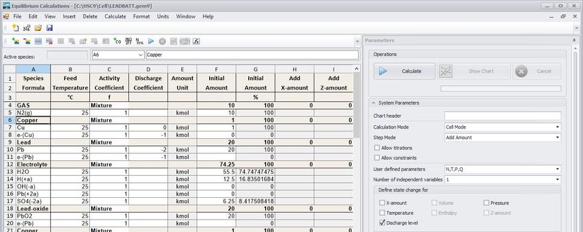
HSC – Equilibrium Module
                                                                                                10/57
                                                                                                Petri Kobylin, Lena Furta, Danil Vilaev

                                                                                                December 11, 2020

               5. Amount of the Species

               In this column user gives the input amounts of the raw material species. The most
               important point for the equilibrium composition is to put the correct amounts of
               elements in the system. User may divide these amounts between the species as user
               likes. If the correct heat balance is required, user must divide the amounts of elements
               exactly into the same phases and in a similar manner as in the real physical world.

               User can choose between mol, kmol or kg/Nm3 units by selecting mol, kmol or kg/Nm3
               from the Units menu. Note that kilograms refer to condensed substances and standard
               cubic meters (Nm3) to gaseous substances.

               6. Amount Step for Raw Materials

               If user wishes to calculate several successive equilibria, user has to give an
               incremental step for one or more raw material species. Then the programs will
               automatically calculate several equilibria by increasing the amount of this species by
               the given step. Please remember to select the Increase Amount option, see Fig. 5, and
               give the number of steps. Some 21 - 51 steps are usually enough to give smooth
               curves to the equilibrium diagram.

               User can give step values for several species simultaneously. For example, if user
               wants to add air to the system, give a step value for both O2(g) and N2(g). Please
               remember to specify the number of steps if a diagram is to be drawn from the results.

               User can also add secondary amount step to plot 3D graphs with different amount
               additions as axis.

               7. Activity Coefficients

               The simple definition of Raoultian activity is the ratio between the vapor pressure of the
               substance over the solution and the vapor pressure of the pure substance at the same
               temperature:

                                                                          (                 )
                                                                     =                                                             (1)
                                                                               (       )

               The activity coefficient describes the deviation of a real solution from an ideal mixture.
               The activity coefficient f is defined as the ratio between activity and mole fraction x of
               the species in the mixture:

                                                                               =                                                   (2)

               In an ideal solution, they are therefore defined as = x and f = 1. As default in Gem
               module, the activity coefficient of a species in the mixture phase is always 1.

               Activity coefficients can be entered as a function of mole fraction of species in the input
               sheet column C. User can choose activity coefficient (f) or natural logarithm of activity
               coefficient (lnf) to column C from Units menu. This Units menu (f or lnf) will change
               units to all phases.

Metso Outotec reserves the right to modify these specifications at any time without prior notice. Copyright © 2021, Metso Outotec Finland Oy
HSC – Equilibrium Module
11/57
Petri Kobylin, Lena Furta, Danil Vilaev
December 11, 2020
Only simple binary or ternary expressions can be utilized directly by the Gem solver
within HSC, such as:
Ln(f) = 8495/T - 2.653
Ln(f) = 0.69 + 56.8·X_24 + 5.45·X_25
Ln(f) = -3926/T
Ln(f) = -1.21·X_7^2 - 2.44·X_8^2
where:
T = Temperature in K
X_24 = Mole fraction (X_) of the species with row number 24 in the sheet.
f = Activity coefficient.
Instead of manually entering the activity coefficient, it is also possible to use pre-
defined activity models. For example, to calculate the activity coefficients with the
Pitzer model using the Aqua module, please select “Aqua” in the solution model drop-
down list when aqueous phase is selected, see Fig. 6. For more information, see
sections 13.4.5, 13.10 and Chapter 36.
Metso Outotec reserves the right to modify these specifications at any time without prior notice. Copyright © 2021, Metso Outotec Finland OyHSC – Equilibrium Module
12/57
Petri Kobylin, Lena Furta, Danil Vilaev
December 11, 2020
13.4. Panel Parameters
Fig. 6. Specifying calculation parameters.
Metso Outotec reserves the right to modify these specifications at any time without prior notice. Copyright © 2021, Metso Outotec Finland OyHSC – Equilibrium Module
13/57
Petri Kobylin, Lena Furta, Danil Vilaev
December 11, 2020
13.4.1. Operations
There are three buttons in this section. Calculate – Equilibrium will be calculated using
the user defined parameters. Show Chart – Diagram will be drawn. Cancel – User can
cancel users last operation.
13.4.2. System Parameters
User may add any kind of heading for the input file, see Fig. 6. The maximum number
of characters allowed in the heading is 80. The program automatically adds the
heading to the diagrams, see Fig. 16.
Default Calculation mode is Normal and Step mode is Add Amount. For advanced
calculation modes see section 13.4.7.
In this section user can specify parameters and define which of them will be changed.
T – Temperature, P – Pressure, N – Amount, V – Volume, H – Enthalpy.
Volume of the system is calculated as sum of volumes of all gaseous phases. User can
select one of the options in the user defined parameters menu. There are
temperature, pressure, and amount in every case, for example, if user selects the N, H,
P system, it means that the temperature will be constant in this system.
Specify a one calculation, 2D or 3D diagram by selecting 0, 1 or 2 in the number of
independent variables, respectively.
Specify, which parameters are changed.
13.4.3. System State
In this section user can specify values or a range of values for the parameters that user
selected above.
If user has defined increments (steps) for raw material species or a specified range for
selected parameters then user should also give the Number of Steps required, see
Fig. 6. Usually 21 - 51 steps give quite smooth curves in the equilibrium diagram. A
large number will only add more points to the diagram and involve a longer calculation
time. It is now also possible to add steps using log mode for each parameter. This is
especially useful when stepping from low to high pressures.
If user has given an amount step for a raw material species, the calculations should be
made using an increasing species amount.
If user checks the Use as base volume option and enter a value for Initial Pressure,
the program will calculate the initial volume and add to it the value for the volume (or
range of values) that user specified earlier.
Metso Outotec reserves the right to modify these specifications at any time without prior notice. Copyright © 2021, Metso Outotec Finland OyHSC – Equilibrium Module
14/57
Petri Kobylin, Lena Furta, Danil Vilaev
December 11, 2020
13.4.4. Calculation Options
Mixing Entropy conversion
HSC converts the entropy values of aqueous components from the molality scale to the
mole fraction scale if the Mixing Entropy conversion for aqueous species option is
selected. Therefore, the entropy values in the results1 sheet are not the same as those
in the HSC database. Identical results will be achieved if the Raoultian activity
coefficients of the aqueous species are changed to 55.509/x(H2O), which converts the
Raoultian activity scale to the aqueous activity scale.
Criss-Cobble
HSC will utilize Criss-Cobble extrapolation for the heat capacity of aqueous species at
elevated temperatures (> 25 °C) if the Criss-Cobble option is selected.
13.4.5. Phase Data - solution models for phases
User first choose the phase where user wants to use a solution model in the system
sheet. Then user choose the solution model from the parameters panel and give the
number of iterations used in the calculations (AC steps). If system consist of Ideal
Mixture and Pure Substance phases only AC step option is disabled.
Ideal Mixture
Default setting for phase is ideal mixture. Gas phase is a typical assumed to behave as
ideal mixture.
Pure Substance (“Invariant phases”)
All species in the phase can be set to be pure substances with the Pure Substance
option, see Fig. 5 and Fig. 6.
Aqua
Aqua modul can be used in aqueous phase. This model uses Pitzer model to calculate
mean activity coefficients of the aqueous species (H2O and species ionic and neutral
species with “a”). User can find the theory of the Aqua solution model in Chapter 36.
Other solution models
There are two solution models available: Ga - As Mixture, Al - Zn Mixture. User can
activate those from Windows menu Add-Ins.
User can find the theory of the solution models and instructions of how to make users
own solution models in section 13.10 for solid and liquid solutions.
It is also possible to enter an activity coefficient formula in column C of the input sheet,
see section 13.3 (numbered list 7. Activity coefficients).
Metso Outotec reserves the right to modify these specifications at any time without prior notice. Copyright © 2021, Metso Outotec Finland OyHSC – Equilibrium Module
15/57
Petri Kobylin, Lena Furta, Danil Vilaev
December 11, 2020
13.4.6. Target Calculations
The idea of the Target Calculations mode is to add a specific constraint to the
general Gibbs Energy Minimization problem and to use a GEM routine to find the point
(with specific pressure, temperature, raw material amounts) at which this constraint is
fulfilled.
Unlike the Constant Volume and Adiabatic calculation modes, the search can be
performed over any valid system parameter (raw material amounts, temperature,
pressure, volume, reaction enthalpy) and the user has to set the search interval
explicitly. The result is a list of system states within the interval that satisfy the
constraint.
For example, user wants to find the temperature where FeSO4·4H2O has an amount of
0.25 kmoles. Enable Target Calculations and set the parameters as in Fig. 7.
Fig. 7. Parameters for Target Calculation mode.
When user presses the Calculate button, the program will make the calculation and
show the results as in Fig. 8.
Metso Outotec reserves the right to modify these specifications at any time without prior notice. Copyright © 2021, Metso Outotec Finland OyHSC – Equilibrium Module
16/57
Petri Kobylin, Lena Furta, Danil Vilaev
December 11, 2020
Fig. 8. Results for Target Calculation mode
13.4.7. Advanced Calculation Options
Default calculation mode is Normal but user can specify other more advanced
calculation modes which are listed here. It is also possible to use different step modes
than Add Amount.
Calculation modes
1. Infinite Phase (Open Atmosphere)
The idea of this calculation mode is to balance the system with the external
environment as a single Gibbs Energy Minimization (GEM) problem.
The system state is termed stationary if the system state does not change in steps.
Metso Outotec reserves the right to modify these specifications at any time without prior notice. Copyright © 2021, Metso Outotec Finland OyHSC – Equilibrium Module
17/57
Petri Kobylin, Lena Furta, Danil Vilaev
December 11, 2020
It is not always possible to find the stationary state for a given system and environment,
because it is possible that some species will accumulate infinitely in the system. For
example, if water steam from the environment is condensed in the system's aqueous
phase, it is possible that the steam will condense infinitely. In such cases the algorithm
will determine these species and consider their molar amount to be infinite, and the
stationary state will be found for the rest of the species.
Note: The selection of the species present in the "open" phase should be made with
caution and only significant species should be added to the open phase. For example,
if zinc vapor is added to the open gas phase at room temperature, it is possible that
solid zinc will fully evaporate, which would appear as an incorrect result in the practical
sense. Of course, zinc evaporation occurs in normal calculations, but is insignificant,
because it would require something like 1030 steps of Transitory Evaporation to
evaporate the zinc.
This mode can be used with some of the other modes. Because the step parameter is
not defined by this mode, it is possible to use T, P, or raw material amounts as a step
parameter in the normal mode; and T, V, P or raw material amounts in the Constant
Volume mode. This mode can be used with the Target Calculations mode. This mode
cannot be used together with the Adiabatic mode.
2. Fixed Activity mode
This section deals with the Fixed Activity Calculation mode. The main idea of this mode
is to fix the activity of some species (corresponding to the molar fraction of that
species) and adjust the initial amount of the species so that this activity constraint is
satisfied at equilibrium.
This mode supports the Constant Volume and Target Calculations modes. This mode
does not support the Transitory Evaporation, Open Atmosphere, Reactor, and
Adiabatic calculation modes.
3. Cell mode
The Cell Equilibrium calculation mode allows calculating equilibrium composition of an
electrochemical cell using the same calculation method as GIBBS-solver. See more in
section 13.9.
Step modes
By checking Allow titrations user can give species concentrations in g/l or mol/l. It is
also possible to give known density of solution (default value is 1 kg/l). If concentration
column is filled, then user gives initial and step amounts in liters for those species and
amount of H2O in that solution is automatically calculated. At same input sheet user
can also give species amounts in normal way using mol, kmol, kg or Nm3 units if
concentration cells are not filled and only amount cells are used, see example file
Allow_Titration.gem9 in Gibbs folder.
Metso Outotec reserves the right to modify these specifications at any time without prior notice. Copyright © 2021, Metso Outotec Finland OyHSC – Equilibrium Module
18/57
Petri Kobylin, Lena Furta, Danil Vilaev
December 11, 2020
1. Final Amount (and Add Amount)
With Final Amount step mode user specifies final amount that is added instead of
amount that is added in each step that is done in Add Amount, which is default step
mode.
2. Remove % (Add Amount or Final Amount)
The idea of this step mode is to balance the system with the external environment step
by step.
Unlike the normal calculation mode, when initial parameters for each step are defined
by the user, in this mode initial parameters are based on the results of the previous
step. Some part of the "open" phase is deleted, initial species are added, and the next
step is calculated.
This calculation mode can be used with some of the other modes. In normal mode, T
and P are fixed across all calculation steps. In the Constant Volume mode, V is fixed
(either defined by the user or calculated based on the initial gas phase amount), and T
or P is adjusted automatically. So, user must choose amount as step parameter.
Please note that this mode cannot be used together with the Target Calculation mode,
because it is impossible to determine intermediate (i.e. between adjacent steps) initial
parameters. Nor can this calculation mode be used together with the Adiabatic mode.
Typical example of Remove % mode is calculation procedure where part of the gas
phase is removed from the chemical system after each calculation step. You can
choose between Remove % (Add amount) and Remove % (Final amount).
3. Reactor
The idea of this Reactor (Standard or Sheets View) step mode is to allow user freedom
to add or remove species (or phases) in each step. It is also possible to change
temperature and pressure in each step. User can for example increase temperature
and decrease temperature in one calculation round (heating and cooling). It is also
possible to give inconstant add amounts of species. With Show AC in each reactor
step option user can specify activity coefficient for each step or specify activity
coefficients just once and those values are used in each step.
Please note that this mode cannot be used together with the Fixed activity mode,
because Fixed activity mode need to know type of phases (pure phases). Nor can this
calculation mode be used together with the Target Calculations.
Typical example of Reactor mode is calculation procedure where part of the gas phase
is removed from the chemical system after each calculation step. You can choose
between
Reactor (Standard) and Reactor (Sheets View).
Metso Outotec reserves the right to modify these specifications at any time without prior notice. Copyright © 2021, Metso Outotec Finland OyHSC – Equilibrium Module
19/57
Petri Kobylin, Lena Furta, Danil Vilaev
December 11, 2020
13.4.8. Examples of the Remove %, Infinite phase and Fixed Activity modes
The system consists of H2O, N2 (g), O2 (g), CO2 (g), and CO2 (a). Initially, only H2O, N2
(g), O2 (g) and CO2 (g) are present in the system; gases are added to the system in
each step, see Fig. 9 - Fig. 15 (for detailed information of these systems, see Chapter
14).
By calculating this system in the step mode Remote % (Add Amount), (Remove
Amount % is here 100 of gas phase - Cell H4 - after each step and re-filling the gas
phase with option), we get the results in Fig. 10.
Fig. 9. Parameters for Remove % mode.
Fig. 10. Diagram for Remove % mode.
Metso Outotec reserves the right to modify these specifications at any time without prior notice. Copyright © 2021, Metso Outotec Finland OyHSC – Equilibrium Module
20/57
Petri Kobylin, Lena Furta, Danil Vilaev
December 11, 2020
By calculating this system in the Infinite Phase mode (calculation option P #1) with
temperature as the step parameter, we get Fig. 11. This chart corresponds to the
expected values of CO2 dissolution from Fig. 10.
Fig. 11. Parameters for Infinite Phase mode.
Fig. 12. Diagram for Infinite Phase mode.
Metso Outotec reserves the right to modify these specifications at any time without prior notice. Copyright © 2021, Metso Outotec Finland OyHSC – Equilibrium Module
21/57
Petri Kobylin, Lena Furta, Danil Vilaev
December 11, 2020
User can also calculate this system in the Fixed Activity mode with a coefficient of
0.0003 for CO2 (g), see Fig. 13.
Fig. 13. Parameters for Fixed Activity mode.
Fig. 14. Diagram with Fixed Activity.
Metso Outotec reserves the right to modify these specifications at any time without prior notice. Copyright © 2021, Metso Outotec Finland OyHSC – Equilibrium Module
22/57
Petri Kobylin, Lena Furta, Danil Vilaev
December 11, 2020
Fig. 15. Activity of CO2(g).
This results in a diagram as in the Infinite Phase mode, see Fig. 14, and user can
check that the Activity for CO2(g) is constant as specified in the Fixed Activity
coefficient, see Fig. 15.
Metso Outotec reserves the right to modify these specifications at any time without prior notice. Copyright © 2021, Metso Outotec Finland OyHSC – Equilibrium Module
23/57
Petri Kobylin, Lena Furta, Danil Vilaev
December 11, 2020
13.5. Diagrams
The diagrams can be drawn, for example, as a function of a specified reactant amount
or equilibrium temperature. User can draw a diagram by pressing Show Chart on the
Parameters Panel or select Chart in the View menu. Gem module now uses same
chart routine as other HSC modules.
User can select species for the axes by clicking the desired button "..." and selecting
the item in the list box using the mouse. The program shows the recommended
selection with an arrow, which is the variable used in the calculations. User can select
a group of species by selecting different phases or/and elements and then selecting the
item from this group.
Fig. 16. 2D diagram.
Metso Outotec reserves the right to modify these specifications at any time without prior notice. Copyright © 2021, Metso Outotec Finland OyHSC – Equilibrium Module
24/57
Petri Kobylin, Lena Furta, Danil Vilaev
December 11, 2020
Fig. 17. Select data for axes.
In this menu user can select the data type for the diagram. Usually user can accept the
default selections by pressing Finish, but the output may be modified. For example,
user can draw the composition of a gas phase by clicking the Equilibrium
Compositions option for the y-axis instead of Equilibrium Amount. All the species in
one phase must be selected if the composition of this phase is to be drawn on the
diagram.
If user is working with an aqueous system, user will be given a pH option for the x-axis.
This option will draw the results as a function of pH.
Temperature and amount units may be selected using the Temperature and Amount
options.
The number of species is not limited, and all the species included in the equilibrium
calculations can be selected for the diagram.
Metso Outotec reserves the right to modify these specifications at any time without prior notice. Copyright © 2021, Metso Outotec Finland OyHSC – Equilibrium Module
25/57
Petri Kobylin, Lena Furta, Danil Vilaev
December 11, 2020
Fig. 18. Select Species.
Fig. 19. 3D diagram.
When user presses Finish in the Axis menu, Fig. 16, the program reads the
equilibrium results and draws the diagram using the default scale, font, line width, etc.
selections, see Fig. 16 and Fig. 19. Note that the program inserts the species labels
automatically above the maximum point of the curve using the same color for the curve
and label. If the line is not within the selected x- and y-range or it is on the border, then
the program will not draw the line or the label.
User can edit the diagram, Fig. 16 and Fig. 19, by using several formatting options:
Double click the x- or y-scale numbers or select X-Axis or Y-Axis from the Format
menu to change, for example, the minimum and maximum values of the x- and y-axes,
Metso Outotec reserves the right to modify these specifications at any time without prior notice. Copyright © 2021, Metso Outotec Finland OyHSC – Equilibrium Module
26/57
Petri Kobylin, Lena Furta, Danil Vilaev
December 11, 2020
see Fig. 20. In some cases, it is also advantageous to change the y-axis to logarithmic
scale to display large variations in amounts or concentrations. From the same window
user can change the number format of x- and y-axis numbers as well as their font size,
color, etc.
1. When the scales are OK, user can relocate any label (species, x- and y-axis
heading, etc.) with the mouse, using the drag and drop method. First select the
label, keep the left mouse button down and drag the label to a new location,
release the mouse button and the label will drop.
2. The line width of curves, species label font, etc. may be changed by double
clicking the species labels or selecting the label with the mouse and selecting
Format Label from the menu. User cannot do this by double clicking the line.
The label and curve editing window is shown in Fig. 21. Note that line styles
other than solid are available only for line widths smaller than 0.3 mm.
3. The walls in a 3D diagram may be changed by selecting Format 3D Diagram
sheet. User can change label, surface, wire frameline, etc, see Fig. 22.
Fig. 20. Changing scales, scale number format and font settings.
Metso Outotec reserves the right to modify these specifications at any time without prior notice. Copyright © 2021, Metso Outotec Finland OyHSC – Equilibrium Module
27/57
Petri Kobylin, Lena Furta, Danil Vilaev
December 11, 2020
Fig. 21. Changing label and line specifications.
Metso Outotec reserves the right to modify these specifications at any time without prior notice. Copyright © 2021, Metso Outotec Finland OyHSC – Equilibrium Module
28/57
Petri Kobylin, Lena Furta, Danil Vilaev
December 11, 2020
Fig. 22. Changing 3D surface specifications.
1. When user is satisfied with the diagram user can print it by pressing Print in top
left corner Chart Menu.
2. If user wants to see the diagram in a tabular format or use the data of the
diagram in other programs, such as MS Excel, press Show menu Table or select
Table Values in top left corner Chart Menu.
3. User can copy the diagram to the Clipboard by pressing Copy as Vector or
Copy as Raster and paste the diagram into other Windows programs. The Copy
command uses the Windows Metafile format, which enables user to resize the
diagram in other Windows applications in full resolution.
4. With Clone user can clone the diagram in a separate file which is outside Gem
module.
Metso Outotec reserves the right to modify these specifications at any time without prior notice. Copyright © 2021, Metso Outotec Finland OyHSC – Equilibrium Module
29/57
Petri Kobylin, Lena Furta, Danil Vilaev
December 11, 2020
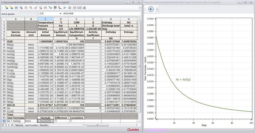
13.5.1. User Formulas
This feature can be activated by clicking formula icon or View…User Formulas.
User Formulas can be used for custom variable visualization, see Fig. 23.
Fig. 23. User Formulas for custom variable visualization.
13.5.2. Toolbar
Drawing additional objects or writing some labels on a diagram can be very helpful in
some cases. User can select one of the shapes (line, arrow, rectangle or circle) or
label, see Fig. 24. If user wants some other shape or label user can use the toolbar
options. User can format the shape by selecting the inner color or border color, line
width, line type. User can make the figure transparent, move to the back or to the front,
see Fig. 24.
User can delete any shape using on the toolbar.
Fig. 24. Toolbar.
Metso Outotec reserves the right to modify these specifications at any time without prior notice. Copyright © 2021, Metso Outotec Finland OyHSC – Equilibrium Module
30/57
Petri Kobylin, Lena Furta, Danil Vilaev
December 11, 2020
Fig. 25. 3D diagram with shapes.
The X and Y labels on the toolbar show the cursor's location. These are only for 2D
diagrams.
13.5.3. Object Editor
Fig. 26. Object Editor of the objects in Fig. 25.
There is one more way to modify diagrams by specifying the coordinates, sizes and
colors of objects in Object Editor. User can Insert, Delete or Edit the shape. To edit
user should change the parameters of the shape. There are two sheets in Object
Editor: Shapes and Labels.
13.5.4. Chart Parameters
The Diagram window appears with the Chart Parameters panel instead of the
Parameters panel. User can use filter options to change the diagram's appearance.
Metso Outotec reserves the right to modify these specifications at any time without prior notice. Copyright © 2021, Metso Outotec Finland OyHSC – Equilibrium Module
31/57
Petri Kobylin, Lena Furta, Danil Vilaev
December 11, 2020
Filter
The main idea of this option is to filter the list of species on the diagram. User can
change this list by selecting different phases and elements. User can select one,
several, or all at once (by selecting "All phases" or "All elements"). The option
"Contains All" means that if user selects several elements, the filter should find only
the species that include all of the selected elements.
Fig. 27. Chart parameters.
Fig. 28. Filtering species in a diagram (AQUA phase chosen here).
Metso Outotec reserves the right to modify these specifications at any time without prior notice. Copyright © 2021, Metso Outotec Finland OyHSC – Equilibrium Module
32/57
Petri Kobylin, Lena Furta, Danil Vilaev
December 11, 2020
Auto Scale
This option helps user to use an appropriate scale when the maximum value of the
diagram's lines is very small. When user unchecks some of the main species, the scale
changes automatically and user can work with lines with smaller values.
Fig. 29. Chart uses automatic scaling when species are filtered (here CO2(a) is unchecked).
Color by Levels
This option allows user to colorize different levels of height charts in different colors.
User can use this option only in a 3D diagram, see Fig. 30.
Fig. 30. Option Color by levels on diagram, see Fig. 19 for comparison.
Metso Outotec reserves the right to modify these specifications at any time without prior notice. Copyright © 2021, Metso Outotec Finland OyHSC – Equilibrium Module
33/57
Petri Kobylin, Lena Furta, Danil Vilaev
December 11, 2020
Show Legend on Chart
This option allows user to add one more panel on a 3D diagram legend panel, see Fig.
31. This panel duplicates the legend on the Chart Parameters panel, so user can check
and uncheck species. The filter also changes it.
Fig. 31. 3D diagram with legend.
Metso Outotec reserves the right to modify these specifications at any time without prior notice. Copyright © 2021, Metso Outotec Finland OyHSC – Equilibrium Module
34/57
Petri Kobylin, Lena Furta, Danil Vilaev
December 11, 2020
13.6. Equilibrium Diagram Tables
User can display the equilibrium results in tabular format by selecting Table Values
(results in columns) in top left corner of the Chart Menu. Other table option is to select
Table (results in rows) in the Show menu in the Diagram window. The Table window
has several Excel-type features in a similar way to the other spreadsheets in HSC. The
most important features are:
1. Copy All puts the whole table on the Clipboard, and pastes this table, for
example, into MS Excel. User can also copy and paste smaller cell ranges using
the Copy and Paste selections in the Edit menu, see Fig. 33.
2. User can also save the table using different formats, such as ASCII text and
Excel by selecting Save from the File menu.
3. The Species sheet contains the data of the diagram; the figures in this sheet can
be edited if user is not satisfied with the results.
There are several formatting options in the Format menu, which can be used to create
representative tables for printing. The table can be printed using the Print selection in
the File menu, Fig. 33. Setup and Preview options are also available for printing.
Fig. 32. Results sheet calculated automatically.
Fig. 33. Equilibrium Diagram Table (Show…Table).
Metso Outotec reserves the right to modify these specifications at any time without prior notice. Copyright © 2021, Metso Outotec Finland OyHSC – Equilibrium Module
35/57
Petri Kobylin, Lena Furta, Danil Vilaev
December 11, 2020
13.7. Restriction of Cp Extrapolation
This feature allows the user to remove the selected species from the calculation if the
system temperature falls outside the temperature range of Cp data for that species. The
Cp data is always given for limited temperature ranges in HSC database. HSC
automatically extrapolates Cp data outside these ranges. Usually this works just fine,
however, in some cases Cp extrapolation may lead to errors. Automatic removal of
species will solve this problem.
The basic approach is as follows: if there are any temperature points at which some of
the species will be outside its defined temperature range, the user is shown the
Warnings window that allows marking of the species to be removed outside its
temperature range.
Note: the old IGI file format does not contain an upper temperature limit for species.
When importing IGI files, the program sets the upper limit to 20000 K.
Plain Calculations
The simplest approach is the normal calculations mode (N, T, P). The Warnings
window uses the temperature range defined in the System State section of the
Parameters panel.
For example, consider the system in NA2SO4.gem9. If the user presses Calculate, the
Warnings window will be shown, see Fig. 35.
Fig. 34. NA2SO4.gem9 test case.
The Warnings windows show all the species that do not have Cp data at least for some
points in the system temperature range. This window allows the user to check the
species that should be deleted outside the defined range. If at some temperature point
the selection requires the deletion of all species containing some element, a message
is shown to the user and the calculation is prevented.
Metso Outotec reserves the right to modify these specifications at any time without prior notice. Copyright © 2021, Metso Outotec Finland OyHSC – Equilibrium Module
36/57
Petri Kobylin, Lena Furta, Danil Vilaev
December 11, 2020
Fig. 35. Warnings window for NA2SO4.gem9 example. Warnings can be disabled or enabled
from “Do not show this dialog” check box.
Fig. 36. Warnings window for NA2SO4.gem9 with species selected for removal.
After the user presses OK, the calculation will begin. The species marked for removal
will be removed outside the available temperature range.
Calculations That Search for Temperature (Adiabatic System)
While in the normal calculation mode (N, T, P) the user defines the temperature range
for the system, there are calculation modes where the temperature range is defined by
the program. In the Constant Volume (N, P, V) and Adiabatic (N, H, P) modes, the
temperature is found by binary search in the range 0 – 20000 K. This means that more
species are subject to extrapolation. The new warnings window handles this by setting
the selected range to 0 – 20000 K. If the user selects a species to be removed, it will
be removed at the search points outside the species temperature range.
Metso Outotec reserves the right to modify these specifications at any time without prior notice. Copyright © 2021, Metso Outotec Finland OyHSC – Equilibrium Module
37/57
Petri Kobylin, Lena Furta, Danil Vilaev
December 11, 2020
In the Adiabatic and Constant Volume modes with base volume calculation, the
temperature of the raw material should be considered. If the temperature of the raw
material lies outside the temperature range for that species, a warning is shown. The
removal of the species in this case is prohibited because it would lead to an illogical
result (the user calculates initial system enthalpy based on data that they consider
incorrect).
Fig. 37. FESO4_adiabatic.gem9 example for adiabatic calculation.
Fig. 38. Warnings for adiabatic calculation.
Metso Outotec reserves the right to modify these specifications at any time without prior notice. Copyright © 2021, Metso Outotec Finland OyHSC – Equilibrium Module
38/57
Petri Kobylin, Lena Furta, Danil Vilaev
December 11, 2020
An example of adiabatic calculation with and without the removal of some species is
presented in Fig. 37- Fig. 40. Without species removal, hydrates begin to form at
temperatures exceeding 4000 °C. The user can prevent this by removing hydrates at
high temperatures, see Fig. 38.
Fig. 39. Adiabatic calculation – without species removal, hydrates are formed at high
temperatures.
Metso Outotec reserves the right to modify these specifications at any time without prior notice. Copyright © 2021, Metso Outotec Finland OyHSC – Equilibrium Module
39/57
Petri Kobylin, Lena Furta, Danil Vilaev
December 11, 2020
Fig. 40. Adiabatic calculation – species “H2O”, “FeSO4*7H2O”, “FeSO4*4H2O”, “FeSO4*H2O”
removed at high temperatures.
Metso Outotec reserves the right to modify these specifications at any time without prior notice. Copyright © 2021, Metso Outotec Finland OyHSC – Equilibrium Module
40/57
Petri Kobylin, Lena Furta, Danil Vilaev
December 11, 2020
13.8. General Considerations
Although equilibrium calculations are easy to carry out with HSC Chemistry, previous
experience and knowledge of the fundamental principles of thermodynamics is also
needed. Otherwise, the probability of making serious errors in basic assumptions is
high.
There are several aspects that should be considered because these may have
considerable effects on the results and can also save a great deal of work. For
example:
1. Before any calculations are made, the system components (elements in HSC Chemistry)
and substances must be carefully defined to build up all the species and substances as
well as mixture phases which may be stable in the system. Phase diagrams and solubility
data as well as other experimental observations are often useful when evaluating
possible stable substances and phases.
2. Defining all the phases for the calculation, which may stabilize in the system, is equally as
important as the selection of system components. User may also select many potential
phases just to be sure of the equilibrium configuration, but this may cause problems in
finding the equilibrium.
3. The definition of mixtures is necessary because the behaviour of a substance (species) in
a mixture phase is different from that in the pure form. The microstructure or activity data
available often determines the selection of species for each mixture. Many alternatives
are available even for a single system, depending on the solution model used for
correlating the thermochemical data.
NB! The same species may exist in several phases simultaneously; their chemical
characteristics in such a case are essentially controlled by the mixture and not by the
individual species.
4. If user expects a substance to exist in the pure form or precipitate from a mixture as a
pure substance, please define such a species in the system as a pure (invariant) phase
also. This is a valid approximation although pure substances often contain some
impurities in real processes. All species in the phase can be set as pure substances
using the Solution model Pure Substance option, see Fig. 6.
5. The raw materials must be given in their actual state (s, l, g, a) and temperature if the
correct enthalpy and entropy values for equilibrium heat balance calculations are
required. These do not affect the equilibrium compositions.
6. Gibbs energy minimization routines do not always find the equilibrium configuration. User
can check the results by a known equilibrium coefficient or mass balance tests. It is
evident that results are erroneous if user obtains a random scatter in the curves of the
diagram. User can then try to change species and their amounts as described in section
13.3. (2. Phases, 5. Amount of Species).
7. Sometimes when calculating equilibria in completely condensed systems it is also
necessary to add small amounts of an inert gas as the gas phase, for example, Ar(g) or
N2(g). This makes calculations easier for the equilibrium programs.
8. It may also be necessary to avoid stoichiometric raw material atom ratios by inserting
an additional substance which does not interfere with the existing equilibrium. For
example, if user has given 1 mol Na and 1 mol Cl as the raw materials and user has NaCl
as the pure substance, all raw materials may fit into NaCl due its high stability. The
routines present difficulties in calculations, because the amounts of all the other phases
and species, except the stoichiometric one, go to zero. User can avoid this situation by
giving an additional 1E-5 mol Cl2(g) to the gas phase.
9. Quite often the simplest examples are the most difficult ones for the Gibbs energy
minimization routines due to matrix operations. For example, the two-phase H2O(g) - H2O
-system between 0 - 200 °C.
Metso Outotec reserves the right to modify these specifications at any time without prior notice. Copyright © 2021, Metso Outotec Finland OyHSC – Equilibrium Module
41/57
Petri Kobylin, Lena Furta, Danil Vilaev
December 11, 2020
10. Sometimes a substance is very stable thermodynamically, but its amount in experiments
remains quite low, obviously for kinetic reasons. User can try to eliminate such a
substance in the calculations to simulate the kinetic (rate) phenomena, which have
been proven experimentally.
11. It is also important to note that different basic thermochemical data may cause
differences in the calculation results. For example, use of HSC MainDB7 or MainDB9
database may lead to different results.
The definition of phases and their species is the crucial step in the equilibrium
calculations and this must be done carefully by the user. The program can remove
unstable phases and substances, but it cannot invent stable phases or species which
have not been specified by the user. The definition of phases is often a problem,
especially if working with an unknown system.
Usually it is wise, as a first approximation, to insert all gas, liquid and aqueous species
into their own mixture phases, as well as such substances which do not dissolve into
them, for example, carbon, metals, sulfides, oxides, etc. into their own invariant phases
(one species per phase), according to basic chemistry. If working with a known system,
it is, of course, clear that the same phase combinations and structural units are
selected for the system as those found experimentally. These kinds of simplifications
make the calculations easier.
The user should give some amount for all the components (elements) that exist in the
system for the Gibbs solver.
It is also important to understand that, due to simplifications (ideal solutions,
pure phases, etc.), the calculations do not always give the same amounts of
species and substances as those found experimentally. However, the trends and
tendencies of the calculations are usually correct. In many cases, when developing
chemical processes, a very precise description of the system is not necessary, and the
problems are often much simpler than, for example, the calculation of phase diagrams.
For example, the user might only want to know at which temperature Na2SO4 can be
reduced by coal to Na2S, or how much oxygen is needed to sulfatize zinc sulfide, etc.
The Na2SO4.gem9 example in the \HSC10\GIBBS directory shows the effect of
temperature on Na2SO4 reduction with coal; the same example can be seen also in the
HSC color brochure, page 3. The calculated compositions are not the same as those
found experimentally, but from these results it can be seen easily that at least 900 °C
will be needed to reduce the Na2SO4 to Na2S, which has also been verified
experimentally.
The real Na-S-O-C-system is quite complicated. To describe this system precisely from
0 to 1000 °C, solution models for each mixture phase would be needed to describe the
activities of the species. Kinetic models would also be necessary at least for low
temperatures. To find the correct parameters from the literature for all these models
might take several months. However, with HSC Chemistry the user can obtain
preliminary results in a matter of minutes. This information is often enough to design
laboratory- and industrial-scale experiments.
Metso Outotec reserves the right to modify these specifications at any time without prior notice. Copyright © 2021, Metso Outotec Finland OyHSC – Equilibrium Module
42/57
Petri Kobylin, Lena Furta, Danil Vilaev
December 11, 2020
13.9. Cell Equilibrium calculations
The Cell Equilibrium calculation mode allows calculating equilibrium composition of an
electrochemical cell using the same calculation method as GIBBS-solver.
The basic definition of an electrochemical system is the same as of a normal system,
with the following additions2,3:
1. For each phase the user must provide its type (gas/liquid/solid/metal), whether it
is an electrode phase (anode or cathode), phase electric capacitance (in Farads)
2. The user must provide discharge equation coefficients and total discharge level
for the system.
Note: in the HSC Cell 7 the capacitance parameter was set as an inverse value of the
actual electric capacitance, with the unit being inverse Farads (F-1). In the new Cell
calculations, the capacitance is set as actual capacitance, with unit being Farads (F).
This conversion is handled automatically when importing an *.ICE file.
To create a new Cell calculation file, the same approach as for normal files is used, but
the menu items with “Cell mode” should be used, like “File -> New -> Empty File (Cell
Mode)”.
Open file menu is the same for both Cell and normal calculations.
C:\Program Files (x86)\HSC10\Cell\LEADBATT.gem9 have been used here as an
example.
The phase and species input in the Cell mode is the same as in normal mode. Once
the phase (or any of the species in it) has been selected, the information in the Phase
Data section on the right is updated (see Fig. 41). Here the user can set the
capacitance (value of 0.00001 is typically used for metals), phase type and electrode
type (if the phase is electrode phase).
Metso Outotec reserves the right to modify these specifications at any time without prior notice. Copyright © 2021, Metso Outotec Finland OyYou can also read