EXPERIMENTAL ASSESSMENT OF IN-DUCT MODAL CONTENT OF FAN BROADBAND NOISE VIA ITERATIVE BAYESIAN INVERSE APPROACH - BEBEC 2020
←
→
Page content transcription
If your browser does not render page correctly, please read the page content below
BeBeC-2020-D20

       EXPERIMENTAL ASSESSMENT OF IN-DUCT
     MODAL CONTENT OF FAN BROADBAND NOISE
     VIA ITERATIVE BAYESIAN INVERSE APPROACH

                          Antonio Pereira1 and Marc C. Jacob1,2
1 Univ   Lyon, École Centrale de Lyon, INSA Lyon, Université Claude Bernard Lyon I, CNRS,
               Laboratoire de Mécanique des Fluides et d’Acoustique, UMR 5509
                  36, Avenue Guy de Collongue, F-69134 Écully Cedex, France
          2 ISAE-SUPAERO, Département d’Aérodynamique Energétique & Propulsion

              10 av. Edouard Belin, B.P. 54032, F-31055 Toulouse Cedex 4, France

                                          Abstract

    Next generation of ultra-high-bypass-ratio (UHBR) engines are associated with an in-
 crease in fan diameter, a reduction of the exhaust jet speed and shorter intake and exhaust
 ducts. A direct impact is that the fan module is expected to be the major noise source
 of commercial aircrafts. It is estimated that the broadband part of fan noise contribution
 fluctuates about 80-90% in approach conditions and about 40% at take-off. Within this
 context, an experimental campaign to characterize fan broadband noise has been conducted
 in the framework of the European project TurboNoiseBB. The experiment has been car-
 ried out at the UFFA fan test rig operated by AneCom AeroTest. Different configurations
 of fan/outlet guide vanes (OGV)-spacing at different working lines have been tested. The
 radiated noise has been measured by in-duct microphone arrays located at the intake, inter-
 stage and downstream of the fan module. A main goal was to assess the modal content of
 fan broadband noise and further estimate the associated sound power levels. This is done
 in the present work via an iterative Bayesian Inverse Approach (iBIA). One outcome of
 this approach is an algorithm allowing to control the sparsity degree of the modal content.
 Thus, different sparsity levels may be tailored to specific noise components (e.g. tonal and
 broadband contributions) based on a priori knowledge. Other advantages are that no as-
 sumption regarding inter-modal correlation is necessary and no parameter has to be tuned
 manually by the end-user.

                                              1
8th Berlin Beamforming Conference 2020                                        Pereira and Jacob

1. INTRODUCTION

In order to face the steady growth of global air traffic, more and more stringent regulations of
noise emissions are imposed. Within an European context, the Advisory Council for Aeronau-
tical Research in Europe (ACARE) has recently confirmed the objective of reducing perceived
noise by 65% relative to the year 2000 (Flightpath 2050). At the same time the bypass ratio
of turbofan engines has been constantly increasing to cope with the goal of reducing fuel burn
consumption. This has lead to the so-called Ultra-High Bypass-Ratio (UHBR) engine architec-
tures. The relative weight of sources contributing to the overall emitted noise has consequently
changed and fan noise is currently responsible of 50% to 65% of the aircraft noise at certifica-
tion points (approach, cutback and sideline). The broadband of that contribution is estimated to
fluctuate about 80% to 90% in approach and about 40% at take-off. Thus reducing fan broad-
band noise has a great potential in reducing aircraft overall noise.
   Within this context an extensive experimental campaign aimed at characterizing fan broad-
band noise and producing reference data for noise predictions has been carried out in the frame-
work of the TurboNoiseBB European Project. Of particular interest in this work are wall-
pressure fluctuations data measured through in-duct phased arrays. One of the goals of Tur-
boNoiseBB is the application of advanced techniques for the analysis of the modal content of
fan broadband noise. Among these an iterative Bayesian Inverse Approach (iBIA) has been ap-
plied. The azimuthal modal content has been assessed both at the intake and the exhaust duct.
In addition the noise at the exhaust duct has been decomposed into wavenumber components
thanks to a linear phased array. This work has allowed the comparison between the noise gen-
erated for two configurations based on different machine geometries. Finally, the estimation of
the duct sound power through a complete decomposition (azimuthal and radial) has been com-
pared to estimations based on azimuthal-only and wavenumber decompositions. It is shown
that a relatively good agreement is obtained between different estimations.

2. OVERVIEW OF THE EXPERIMENTAL TEST CAMPAIGN

An experimental campaign to characterize fan broadband noise has been carried out in the
framework of the TurboNoiseBB project. The experiment has been carried out at the UFFA
fan test rig operated by AneCom AeroTest. An extensive database of both acoustic [5, 22] and
aerodynamic data [15] has been acquired. A sketch of the ducted test-section in Figure 1(a)
depicts the position of mode detection rings relative to the fan. Of particular interest for the
present work are the azimuthal ring CMD1 at the intake, as well as the azimuthal ring CMD3
and the axial line array (AX1) both at the bypass section downstream of the Outlet Guide Vanes
(OGV).
   The tested fan has 20 blades and a diameter of about 34 inches. A set of 44 OGVs is used at
two different machine configurations. A first one with a nominal gap between fan and OGVs
and a second one with increased fan-OGV distance. The first configuration is called hereafter
Short-Gap (SG) and the latter is referred to as Long-Gap (LG). The measurements have been
acquired at different rotational speeds for two working lines. The first one being a sea level
static working line (SLS-WL) and the second one a low noise working line (LNWL).

                                               2
8th Berlin Beamforming Conference 2020                                                   Pereira and Jacob

                                  (a)                                               (b)

Figure 1: (a) Sketch of the test-bench showing the different mode detection arrays and (b) a
          photo showing the intake with the turbulence control screen (TCS) installed.

2.1. Description of the microphone arrays

The test bench has been equipped with various mode detection rings. The goal was to char-
acterize the modal content at the intake, inter-stage and at the by-pass section downstream of
OGVs. The intake is equipped with a ring of about 100 kulite R XCS-190 pressure transducers
distributed non-uniformly along the duct circumference. This configuration allows to capture
the azimuthal modal content up to an azimuthal order of m = ±79 without aliasing.
   The bypass duct is equipped with a combination of a mode detection ring (CMD3) and an
axial linear array (AX1). The azimuthal ring is equipped with about 100 Endevco R 8510C
piezoresistive pressure transducers. As for the CMD1 array, the probes are non-uniformly dis-
tributed along the outer duct casing, allowing a decomposition up to azimuthal order m = ±79.
The axial linear array is composed of 60 G.R.A.S R 40BP pressure microphones. The array
axial extent is about 0.8D with D the duct diameter and the microphone inter-spacing is of the
order of a cm.

3. OUTLINE OF THEORY

This section is organized into three main parts. In the first one a description of the in-duct pres-
sure field using a modal approach is detailed. In the second part, the mode detection problem
is formulated using a matrix notation. Finally, the method used to solve the mode detection
problem is briefly described.

3.1. Modal description of in-duct pressure field

The acoustic pressure p(z, r, φ ) inside a hard-wall cylindrical duct may be conveniently decom-
posed as a weighted sum of modes [17]:
                                    ∞   ∞h                           i
                                            +     + z
                                                jkm,n    −       − z
                                                               jkm,n
                  p(z, r, φ ) =    ∑      A
                                        ∑ m,n e       + Am,n e         fm,n (r)e jmφ ,                 (1)
                                  m=−∞ n=0

                                                    3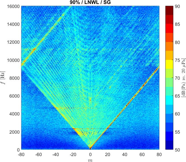
8th Berlin Beamforming Conference 2020                                             Pereira and Jacob

with A+            −
         m,n and Am,n the complex-valued coefficients of modes propagating downstream and up-
stream respectively. The subscripts m and n are the azimuthal and radial mode orders. The
terms km,n± are the axial wavenumbers in both downstream (+ ) and upstream (− ) directions and

 fm,n (r) is a normalized modal shape factor which depends on the duct’s cross section and radial
boundary conditions. Expressions for the modal shape factor for both circular and annular duct
sections are given in Appendix A. Mode axial wavenumbers km,n  ± are in turn given by

                                       ±          Mz
                                      km,n =−        k0 ± k̂r,m,n ,                               (2)
                                                  β2

with Mz = U0 /c the Mach number along the z direction, β 2 = 1 − Mz2 the squared
Prandtl–Glauert factor and k0 = ω/c the acoustic wave number. The term k̂r,m,n is then written
                                           1
                                             q
                                 k̂r,m,n = 2 k02 − β 2 kr,m,n
                                                        2     ,                             (3)
                                          β
where kr,m,n is a radial or transversal wavenumber whose value depends on the boundary con-
ditions at the duct walls, i.e. at r = rh and r = rt (see Figure 2). The modeling of the in-duct
acoustic pressure through Eq. (1) requires the knowledge of physical quantities such as the
mean flow speed and sound speed that in turn depends on the temperature. From an experimen-
tal point of view, these values must be accurately measured to ensure an accurate model of the
pressure field. Simplifications of Eq. (1) are an interesting approach to avoid this requirement
while leading to valuable information. For instance, Eq. (1) may be written as
                                              ∞
                                   p(φ ) =    ∑      Cm (z0 , r0 )e jmφ ,                         (4)
                                             m=−∞

that decomposes a spatial pressure field onto an azimuthal basis with associated azimuthal mode
coefficients Cm (z0 , r0 ). Notice that these coefficients represent the sum over radial orders n from
Eq. (1). Thus, the contribution of both downstream A+                             −
                                                              m,n and upstream Am,n modes is intrin-
sically represented in Cm (z0 , r0 ). This is indeed one limitation of this simplification, that is,
the contribution of both downstream and upstream propagating modes may not be separated.
The dependency of Cm on (z0 , r0 ) has been made explicit to emphasize that this decomposition
must be carried out at constant axial and radial positions in the duct. For instance, for a ring
of acoustic pressure measurements. Another simplification of very practical interest is the de-
composition of the in-duct pressure field into its wavenumber components. This can be written
as
                                              ∞
                                   p(z) =    ∑       Dkz (r0 , φ0 )e jkz z ,                      (5)
                                            kz =−∞

where z is the axial coordinate along the duct axis, r0 and φ0 are constant radial and azimuthal
coordinates and Dkz are the amplitude coefficients of wavenumber components kz . In prac-
tice, due to the limited spatial sampling of linear arrays, aliasing will occur and the maximum
wavenumber recovered without ambiguity is kzmax = π/∆z , ∆z being the minimum separation
distance between microphones. Another limitation concerns the resolution in the wavenumber

                                                     4
8th Berlin Beamforming Conference 2020 Pereira and Jacob
domain which is limited by the spatial extent of the array and is given by ∆kz = 2π/Lz , with
Lz the array length. Setting the values of wavenumber components kz from negative to positive
values allows to separate waves propagating along both upstream and downstream directions. In
addition hydrodynamic components, associated to turbulent boundary layer noise for instance,
may also be separated. These are main advantages of this approach. Finally, all presented for-
mulations may be written using a matrix-vector formulation. This is the subject of the next
section.
y
p
x Amn- U0
r
ϕ
z A+mn
r=rt r=rh
Figure 2: Sketch of the cylindrical coordinates system used in the problem.
3.2. Discussion on the mode detection problem
In order to characterize the in-duct modal content, one approach is to sample the acoustic pres-
sure within the duct and try to estimate the associated complex-valued mode amplitudes. In
other words the idea is to discretize the left hand side of Eqs. (1), (4) or (5) and solve for the
respective coefficients A±m,n , Cm and Dkz . For implementation purposes the infinite sums must
be truncated, the highest azimuthal order is set to M and highest radial order set to N for in-
stance. A linear system of equations is set between all K measurement positions and all mode
coefficients. A matrix-notation version of Eq. (1)is written as
p = Φc, (6)
with p ∈ CK a vector of complex-valued measured pressure at a given frequency ω and c ∈ CL
a vector containing the complex modal coefficients A+ −
m,n and Am,n . The dimension L depending
on the number of considered azimuthal (M) and radial (N) modes. The matrix Φ ∈ CK×L is
filled with the corresponding terms of the modal basis. The goal is to solve this equation for
the mode coefficients c. Whenever the assumption of stationarity and ergodicity of time signals
holds, the expression in Eq. (6) may be conveniently written in terms of the cross-spectral
matrix of measurements, written by definition as Spp , E{ppH }. The notation ·H representing
the conjugate transpose or the Hermitian of a vector and E{·} to be understood as the expected
value over the number of snapshots. Equation (6) then reads
Spp = ΦScc ΦH , (7)
with Scc , E{ccH } the cross-spectral matrix of modal coefficients. The quantity of interest is
often the squared value of mode amplitudes, which are simply given by the diagonal terms of
Scc . Off-diagonal terms are the cross-spectra between modal coefficients and may be of interest
58th Berlin Beamforming Conference 2020 Pereira and Jacob
in cases where mutual coherence between modes is expected, for instance at tonal frequencies.
Several techniques and algorithms [12, 14] exist to solve the problem in Eq. 7, either solving for
each mode coefficient independently, such as beamforming, or solving the problem as a whole,
such as inverse methods.
One typical implementation of beamforming is known as Least-Squares Beamforming [21],
the solution for mode coefficients is written as
φH
l Spp φl
ĉl = , (8)
kφl k
where φl is the l-th column of matrix Φ and ĉl is the l-th entry in the diagonal of the cross-
spectral matrix of modal coefficients Ŝcc . The off-diagonal terms of Ŝcc are by definition van-
ishing, due to the assumption that modal coefficients are mutually incoherent. The advantages
of beamforming are its robustness and computational speed. However, a limited resolution and
poor quantification results are well-known limitations of beamforming. Inverse methods and
deconvolution approaches are alternatives to overcome beamforming limitations at the expense
of a higher computational cost. An iterative Bayesian Inverse Approach (iBIA) is applied in the
present work. This method has been recently applied to the localization and quantification of
aeroacoustic sources, such as jet noise [12] and airframe noise [4, 14]. Theoretical aspects of
iBIA are briefly recalled in the next section.
3.3. Overview of the iterative Bayesian Inverse Approach (iBIA)
The idea behind the Bayesian framework applied to inverse problems [2] is to model all un-
knowns of the problem as random variables. A probabilistic distribution is then assigned to
random variables through probability density functions (PDFs). The optimal choice of PDFs
will be guided based on a priori assumptions and available knowledge of the problem by the
user. A significant advantage of the Bayesian approach to ill-posed inverse problems is the
generation of tailored regularization techniques [19]. An extensive investigation on different
PDFs for the inverse acoustic problem has been recently presented by Antoni et al. [3]. It
can be shown that the modeling of unknown variables, in the present work c, by a generalized
multivariate complex Gaussian distribution leads to the following minimization problem [11]
ĉ = Argmin kp − Φck22 + η 2 kck pp ,
(9)
where by notational convention kck pp = ∑N p
i=1 |qi | is defined as the ` p -norm of the vector c. The
choice of p = 2 leads to the classical Tikhonov regularized solution. Other choices of p may be
used to control the degree of sparsity of the solution, in particular p < 2 is of interest. A study
on different choices of p has been done for the problem of noise source localization [11]. No
closed-form solution of Eq. (9) exists for values of p < 2 since the minimization problem is
not quadratic. In this case the Majorization-Minimization (MM) principle [9] may be used to
solve it. This leads to an iterative algorithm at which a quadratic function is minimized at each
iteration [12, 18]. The resulting algorithm is within the family of Iterative Reweighted Least
Squares (IRLS) algorithms [6]. In the following sections a value of p = 1 is set for solving the
mode detection problem from Eq. (7). Two worth to mention advantages of this approach are:
first that no assumption regarding mode inter-correlation is done a priori and second that no
68th Berlin Beamforming Conference 2020 Pereira and Jacob
further parameters have to be set by the user since the regularization procedure is automated.
4. RESULTS & DISCUSSION
4.1. Single-out fan broadband noise through cyclostationary tools
In order to focus the analysis on fan broadband noise a technique to separate tonal and broad-
band noise has been applied to the measured data [1]. A tachometer trigger one-pulse per
revolution signal has allowed an angular resampling of wall-pressure time signals. This step
ensures a regular number of time samples per rotor revolution. Resampled data is then averaged
over one or more rotor cycles, depending on the required angular frequency resolution. The
deterministic signal obtained in the previous step is then subtracted from raw angular signals.
The result is a residual signal whose 1st order cyclo -stationary has been removed. This residual
signal contains 2nd and higher order cyclo-stationary components. An example of spectra ob-
tained after this procedure is shown at Fig. 3. Unless otherwise stated, mode detection results
shown in upcoming sections have been obtained with data following tone extraction.
0 50 100 150 200 250
Figure 3: Example of wall-pressure fluctuations spectra measured at the bypass duct mode de-
tection ring (CMD3) that illustrates the separation between tonal and broadband
noise. Results show the raw power spectral density (PSD) in black, the rotor-locked
tonal noise PSD in gray and the residual spectrum containing the broadband part of
measured signals in red. Results are representative of cutback power with a fan speed
of 80%ND.
4.2. Intake azimuthal mode plots versus power
The azimuthal modal content at the intake is computed through Eq. (4) with data from mi-
crophone ring CMD1, see Figure 1(a). The results are presented as 2D color plots of mode
amplitudes versus frequency. Figure 4 shows the results for the short-gap fan-OGV configu-
ration at the sea level static (SLS) working line. The azimuthal modal content is shown as a
function of power at the three certification points, namely: approach (50% ND), cutback (80%
ND) and sideline (90% ND). Notice that tonal components have been extracted following the
procedure from Sec. 4.1.
78th Berlin Beamforming Conference 2020 Pereira and Jacob
The structure of mode plots is seen to vary considerably with the increase of fan speed. In par-
ticular, a clear change in behavior is observed above 80%, the modal energy tends to be highly
concentrated along the cut-on/cut-off boundary. This change in modal structure is more re-
markable for the mode plots at the low noise working line (LNWL), see Fig. 5(c). This effect is
likely to be related to the generation of shock waves at the rotor blades for transonic/supersonic
tip speeds. These shock waves are known to block the passage of downstream generated noise
over the fan blades. This might explain the energy reduction at low frequencies observed for
the 90% case. At approach power the modal energy is higher at low frequencies up to about 5
kHz. Common to the three tested speeds is a bias towards positive spinning orders m, which are
co-rotating modes in the reference frame used here.
An aliasing of co-rotating mode amplitudes onto negative azimuthal orders m is observed
at frequencies above 10 kHz. This is related to the azimuthal order limit given by the array
geometry, see Sec. 2.1. As the speed increases the occurrence of aliased content is shifted
towards lower frequencies.
(a) (b) (c)
Figure 4: Azimuthal mode detection plots at the intake as a function of engine power. Results are
given for three operating points, namely: (a) approach 50%ND, (b) cutback 80%ND
and (c) sideline 90%ND. Results are for the short gap rotor/stator configuration at
the sea level static working line (SLS-WL).
In order to quantify the bias towards co-rotating modes for intake mode spectra, the modal
amplitudes are integrated over both co-rotating and counter-rotating modes. The resulting spec-
tra are shown at Fig. 6 for approach and cutback power. At lower fan-speeds the gap between
co- and counter-rotating modes is significant, see Fig. 6(a). Also noticeable at these spectra
are several spectral humps which are not exactly centered at BPF tones. These humps are also
present at cutback power, see Fig. 6(b), although they are more spaced apart over frequency
and the spectral broadening is wider. Similar behavior of inlet duct wall-pressure spectrum
have also been observed elsewhere, see Ref. [8]. It is argued therein that this spectral content
might be related to rotor interaction with inlet boundary layer. As the fan speed increases, the
level difference between co-rotating and counter-rotating modes is reduced, see Fig. 6(b).
88th Berlin Beamforming Conference 2020 Pereira and Jacob
(a) (b) (c)
Figure 5: Azimuthal mode detection plots at the intake as a function of engine power. Results are
given for three operating points, namely: (a) approach 50%ND, (b) cutback 80%ND
and (c) sideline 90%ND. Results are for the short gap rotor/stator configuration at
the low noise working line (LNWL).
50% / HNWL / SG 80% / HNWL / SG
95 110
105
90
100
85 95
90
80
85
75 80
0 1 2 3 4 5 6 7 8 9 10 0 1 2 3 4 5 6 7 8 9 10
(a) (b)
Figure 6: Integrated intake mode spectra over co-rotating (+m) and counter-rotating (−m)
modes for two fan speeds: (a) approach 50%ND and (b) cutback 80%ND. The results
are given for the short fan-OGV gap at the sea level static working line (SLS-WL).
4.3. Bypass-duct azimuthal mode plots versus power
The azimuthal mode content at the bypass duct downstream of OGVs is shown in Fig. 7 for
increasing engine power. The results are obtained using the data from the downstream mode
detection ring CMD3, see Fig. 1(a). It can be noticed that contrary to intake mode plots no clear
bias towards co- or counter-rotating modes exists. A slight bias towards counter-rotating modes
is noticeable for modes well above cut-on, however. As frequency increases the energy of mode
plots tends to be rather concentrated on modes well above cut-on, with lower azimuthal orders.
The general modal structure does not change drastically with increasing power, as compared to
intake mode plots. However, the modal energy is seen to gradually increase from lower (see
approach) to higher speeds (cutback and sideline). The effect of aliasing is not clearly seen as
98th Berlin Beamforming Conference 2020 Pereira and Jacob
compared to intake mode plots. This is because pressure levels are much lower for modes close
to the cuton/cutoff boundary.
(a) (b) (c)
Figure 7: Azimuthal mode detection plots at the bypass duct as a function of engine power. Re-
sults are given for three operating points, namely: (a) approach 50%ND, (b) cutback
80%ND and (c) sideline 90%ND. Results are for the short gap rotor/stator configu-
ration at the sea level static working line (SLS-WL).
The azimuthal mode detection maps have been integrated over both co-rotating and counter-
rotating modes. Resulting spectra are shown in Fig. 8 at approach and sideline power. Com-
pared to intake mode spectra, see Fig. 6, the levels are more evenly balanced between co-
rotating and counter-rotating modes. As frequency increases, however, a bias towards counter-
rotating modes is observed for both approach and sideline power. The level difference is of the
order of 3 dB.
50% / HNWL / SG 90% / HNWL / SG
100 110
95 105
90 100
85 95
80 90
0 1 2 3 4 5 6 7 8 9 10 0 1 2 3 4 5 6 7 8 9 10
(a) (b)
Figure 8: Integrated bypass mode spectra over co-rotating (+m) and counter-rotating (−m)
modes for two fan speeds: (a) approach 50%ND and (b) sideline 90%ND. The results
are given for the short fan-OGV gap at the sea level static working line (SLS-WL).
108th Berlin Beamforming Conference 2020 Pereira and Jacob
4.4. Wavenumber decomposition at the bypass-duct
The test bench is equipped with a linear microphone array at the bypass-duct downstream of
OGVs, as outlined in Sec. 2.1. Several post processing techniques may be applied using this
kind of array geometry, in duct beamforming [13, 24] and wavenumber decompositions are
common examples [7, 20, 22]. In the present work a wavenumber decomposition is performed
through the formulation given by Eq. (5). Figure 9 shows the wavenumber domain spectra at
different fan speeds, namely: approach, cutback and sideline. Few remarks are of importance
for the interpretation of results. First, aliased wavenumber components are clearly seen on the
2D color plots. These are due to the limited inter-microphone axial separation distance, which
is of the order of a cm. Two types of aliased data are apparent. The first one is related to the
hydrodynamic-associated component with a slope dependent on the velocity at which turbulent
structures are convected downstream. The aliased data appear at the negative wavenumber do-
main at frequencies around 3 to 5 kHz, depending on the fan speed. When aliased data overlaps
the acoustic domain, care should be taken to interpret results. A second type is related to the
aliasing of upstream acoustic components (negative wavenumbers) into the positive wavenum-
ber domain. This contribution arises at higher frequencies, tipycally above 10 kHz. A clear
separation between acoustic and hydrodynamic components is obtained, except at very low
frequencies. Notice the inclination of the “V-shaped” acoustic domain in the anti-clockwise di-
rection due to the convective effect of the mean flow. The inclination increases with increasing
fan speed. The structure of wavenumber decomposition plots is rather similar for all tested fan
speeds, with most energy concentrated on positive wavenumber domain, that is, sound propa-
gating downstream in the duct. The “U-shaped” structures apparent at the acoustic domain data
are related to the axial wavenumber of duct modes, see Eq. (2).
(a) (b) (c)
Figure 9: Wavenumber decomposition plots obtained at the bypass-duct as a function of engine
power. Results are given for three operating points, namely: (a) approach 50%ND,
(b) cutback 80%ND and (c) sideline 90%ND. Results are for the short gap rotor/stator
configuration at the sea level static working line (SLS-WL).
118th Berlin Beamforming Conference 2020 Pereira and Jacob
4.5. Influence of the fan/OGV separation distance
As mentioned in Sec. 2 two different fan-OGV inter-spacings have been tested during the
TNBB experimental campaign. In this section, a comparison is made between both configura-
tions using in-duct wall-pressure fluctuations data. In particular, the modal content estimated
through the different microphone arrays will be used for the analysis. The influence on the noise
measured at both intake and bypass-duct is assessed.
Noise measured at the intake duct
Azimuthal mode detection plots for both the short-gap (SG) and long-gap (LG) OGV config-
urations are shown in Fig. 10. The structure of mode plots do not change considerably when
comparing LG and SG configurations at the fan speeds of 50%ND and 60%ND. Although lev-
els for positive spinning modes are slightly higher for the SG. Looking at mode plots estimated
at 100%ND, see Figs. 10(c) and 10(f), a significant level increase on positive spinning modes
close to cut-off is noticed for the SG configuration.
In order to ease the comparison, mode pressure levels are integrated over both co-rotating
and counter-rotating mode amplitudes as done in previous sections. Integrated mode spectra
at approach power are shown in Fig. 11(a). As can be seen, the conclusions differ for co-
rotating or counter-rotating mode spectra. For the first, pressure levels for both SG and LG are
equivalent from low frequencies up to 2 kHz. As frequency increases, the LG configuration
shows pressure levels at the order of 3dB lower than the SG configuration. For the counter-
rotating pressure spectra, no difference is observed between SG and LG configurations over
the whole frequency band. This result suggests that the source mechanism at the origin of this
counter-rotating intake noise is not altered by the presence of the stator behind the rotor, that
would be the case of rotor interaction with inlet boundary layer. On the other hand, co-rotating
mode spectra suggests that the source mechanism is an interaction between fan and OGV. The
results at 60%ND fan speed indicate that the noise reduction of LG configuration reduces as
the fan speed increases. One possible explanation is that the balance between different noise
sources is changed with increasing speed.
Noise measured at the bypass-duct
The influence of fan-OGV separation distance on the noise at the bypass-duct is assessed in Fig.
12 for the approach condition. The trends are quite similar for both co-rotating and counter-
rotating mode spectra. The long-gap OGV configuration leads to relatively higher levels at
lower frequencies and a reduction of noise at higher frequencies. The noise reduction seems to
be more important for counter-rotating modes, see Fig. 12(b). This observation is in agreement
with the argument that a larger separation allows a reduction of turbulent wake intensity, a
widening of wakes and an increase of turbulence length scales. The intensity reduction would
lead to a decrease of noise levels. The increase of length scales would lead to an increase of
levels at low frequencies and a reduction at high frequencies.
Different observations are found for increasing fan rotational speeds, as seen in Fig. 13 at
sideline power. In this case the frequency band at which levels are increased for LG configura-
tion are even wider, up to about 8 kHz.
128th Berlin Beamforming Conference 2020 Pereira and Jacob
(a) (b) (c)
(d) (e) (f)
Figure 10: Influence of the fan-OGV separation distance on the azimuthal mode content esti-
mated at the intake duct. Top row: long-gap OGV results; Bottom row: short-gap
OGV results. Mode plots are shown for the following three fan speeds at the SLS-
WL: (a,d) 50%ND; (b,e) 60%ND and (c,f) 100%ND.
4.6. Estimation of the duct sound power
The decomposition of in-duct pressure field into azimuthal and radial modes, see Eq. (1), allows
for a direct computation of the duct sound power [16]. The relation between mode acoustic
power and modal amplitudes are given by the following equation:
± πk0 β 4 k̂r,m,n 2
Wmn = A±
m,n , (10)
Z0 k0 ∓ Mz k̂r,m,n
with Z0 = ρ0 c the acoustic impedance and k̂r,m,n as given by Eq. (3). Equation (10) gives the
sound power carried by each individual mode Wmn . The total transmitted sound power along
the duct is often of interest. The integration of Eq. (10) over azimuthal and radial mode orders
138th Berlin Beamforming Conference 2020 Pereira and Jacob
95 110
105
90
100
95
85
90
85
80
80
75 75
0 1 2 3 4 5 6 7 8 9 10 0 1 2 3 4 5 6 7 8 9 10
(a) (b)
Figure 11: Intake mode spectra integrated over co-rotating (+m) and counter-rotating (−m)
modes both the short-gap and long-gap OGV configurations. Results are shown for
two fan speeds: (a) 50%ND and (b) 60%ND.
100 100
95 95
90 90
85 85
80 80
0 1 2 3 4 5 6 7 8 9 10 0 1 2 3 4 5 6 7 8 9 10
(a) (b)
Figure 12: Influence of the fan-OGV separation distance on the noise measured at the bypass-
duct at approach power. Figure shows integrated mode amplitudes for SG and LG
configurations for: (a) co-rotating modes and (b) counter-rotating modes.
gives the total in-duct sound power transmitted either downstream W + or upstream W − :
πk0 β 4 M N k̂r,m,n 2
W± = ∑ ∑ A±
m,n , (11)
Z0 m=−M n=0 k0 ∓ Mz k̂r,m,n
where M and N are respectively the maximum azimuthal and radial orders considering only
cut-on modes. Often it is not possible to obtain a complete modal breakdown since it requires a
relatively large number of microphones distributed over azimuthal and axial positions. It is of
interest thus to obtain an estimate of in-duct sound power based on azimuthal-only or wavenum-
ber decompositions. Although this requires an assumption regarding the distribution of the
modal energy. This has been investigated by Joseph et al. [10], where different assumptions on
the modal distribution have been studied. An assumption which is commonly adopted for fan
broadband noise is the Equal Energy Density per Mode (EEDM). This is the assumption tested
here for the computation of duct sound power based on both azimuthal-only and wavenum-
148th Berlin Beamforming Conference 2020 Pereira and Jacob
110 110
105 105
100 100
95 95
90 90
0 1 2 3 4 5 6 7 8 9 10 0 1 2 3 4 5 6 7 8 9 10
(a) (b)
Figure 13: Influence of the fan-OGV separation distance on the noise measured at the bypass-
duct at sideline power. Figure shows integrated mode amplitudes for SG and LG
configurations for: (a) co-rotating modes and (b) counter-rotating modes.
ber decompositions. These estimations are then compared to sound power computed directly
through Eq. (11). Results of the comparison are shown in Fig. 14 for two operating points
representative of approach and cutback power. The different estimations agree relatively well
over the whole frequency band. The sound power estimated from azimuthal-only decomposi-
tion at low frequencies are several dB’s higher than the others. This trend is seen to increase
with increasing fan speed. This result is somewhat expected since azimuthal-only decompo-
sition (AMD) does not allow the separation between downstream and upstream propagating
modes. This would lead to an overestimation of levels. In addition, the results from both AMD
and ARMD (azimuthal and radial modal decomposition) may be corrupted by hydrodynamic-
associated noise at low frequencies. On the other hand, the wavenumber decomposition (WND)
allows to filter-out this contribution.
50% / HNWL / SG 80% / HNWL / SG
110 110
100 100
90 90
80 80
70 70
0 1000 2000 3000 4000 5000 6000 7000 8000 9000 10000 0 1000 2000 3000 4000 5000 6000 7000 8000 9000 10000
(a) (b)
Figure 14: Comparison between different estimations of the in-duct sound power at the bypass-
duct. ARMD: Azimuthal and Radial Modal Decomposition, WND: Wavenumber
Decomposition-based and AMD: Azimuthal Modal Decomposition-based. Results
are given for the sea level static working line and for the short-gap OGV configura-
tion at (a) approach 50%ND and (b) cutback 80%ND.
158th Berlin Beamforming Conference 2020 Pereira and Jacob
5. CONCLUSIONS
Fan broadband noise is responsible for a major part of aircraft overall noise for future UHBR
engine architectures. To improve understanding of its generation mechanisms an extensive
experimental database has been acquired within the TurboNoiseBB project. The present work
has been focused in the analysis of broadband noise at both the intake duct and the bypass
section of a rotor/stator stage.
Azimuthal mode detection and wavenumber decomposition of wall-pressure fluctuations data
have been computed. The application of an iterative Bayesian Inverse Approach (iBIA) has
allowed results with improved dynamic range and limited aliasing by the introduction of sparsity
enforcing constraints.
A short-gap and a long-gap OGV configuration have been compared in terms of the noise
generated both at the intake and the bypass duct. Increasing the rotor-stator spacing has shown
reduced levels at higher frequencies for intermediate fan speeds (see approach) for both inlet
and exhaust noise. With increasing fan speed the difference between SG and LG configurations
tends to decrease and LG even showing higher levels for exhaust noise at low frequencies.
Although, it is important to mention that the fan was not designed to work on a LG build and
the same OGV set has been used for both configurations. In addition a modification of the duct
casing has been done for the LG mounting.
The in-duct sound power has been estimated through three different approaches. One based
in a complete modal breakdown and other two requiring an assumption on the modal distribu-
tion. A good agreement between these approaches has been found mainly at medium to high
frequencies using a Equal Energy Density per Mode distribution. The agreement at low fre-
quencies is hindered by the presence of strong hydrodynamic disturbances due to the flow and
the impossibility to separate downstream and upstream modes for the azimuthal-only decom-
position. These results supports the assumption of EEDM distribution commonly used for fan
broadband noise.
Acknowledgements
The presented work was conducted in the frame of the project TurboNoiseBB, which has re-
ceived funding from the European Union’s Horizon 2020 research and innovation program un-
der grant agreement No. 690714. It was also performed within the framework of the Labex
CeLyA of the Université de Lyon, within the program ”Investissements d’Avenir” (ANR-10-
LABX-0060/ANR-16-IDEX-0005) operated by the French National Research Agency (ANR).
The authors kindly acknowledge all the team from TurboNoiseBB involved in the test cam-
paign.
168th Berlin Beamforming Conference 2020 Pereira and Jacob
A. Normalized mode shape factors
A.1. Circular cross section
The normalized modal shape factor for a circular duct (see Ref. [23]) may be written as:
J|m| (kr,m,n r)
fm,n (r) = , (12)
Γm,n
with kr,m,n a radial or transversal wavenumber whose value depends on the boundary condition
at the duct wall, J|m| (·) is the m-th order Bessel function and Γm,n is a normalization factor
introduced to ensure that the modal shape functions are orthonormal, that is, orthogonal and
normalized over the duct’s cross section.
A.2. Annular cross section
The radial shape factors for an annular duct may be expressed as
1
fm,n (r) = J|m| (kr,m,n r) +CY|m| (kr,m,n r) , (13)
Γm,n
with J|m| (·) and Y|m| (·) the m-th order Bessel and Neumann functions respectively and the coef-
ficient C is given by
0 (k
J|m| r,m,n rt )
C=− 0 , (14)
Y|m| (kr,m,n rt )
0 (·) and Y 0 (·) the first derivatives of Bessel and Neumann functions and r the radius
with J|m| |m| t
at the outer duct casing.
References
[1] J. Antoni. “Cyclostationarity by examples.” Mechanical Systems and Signal Processing,
23(4), 987 – 1036, 2009.
[2] J. Antoni. “A bayesian approach to sound source reconstruction: Optimal basis, regulariza-
tion, and focusing.” The Journal of the Acoustical Society of America, 131(4), 2873–2890,
2012.
[3] J. Antoni, T. L. Magueresse, Q. Leclère, and P. Simard. “Sparse acoustical holography
from iterated bayesian focusing.” Journal of Sound and Vibration, 446, 289–325, 2019.
[4] C. J. Bahr, W. M. Humphreys, D. Ernst, T. Ahlefeldt, C. Spehr, A. Pereira, Q. Leclère,
C. Picard, R. Porteous, D. Moreau, J. R. Fischer, and C. J. Doolan. “A comparison of
microphone phased array methods applied to the study of airframe noise in wind tunnel
testing.” In 23rd AIAA/CEAS Aeroacoustics Conference. American Institute of Aeronau-
tics and Astronautics, 2017.
178th Berlin Beamforming Conference 2020 Pereira and Jacob
[5] M. Behn and U. Tapken. “Investigation of sound generation and transmission effects
through the ACAT1 fan stage using compressed sensing-based mode analysis.” In 25th
AIAA/CEAS Aeroacoustics Conference. American Institute of Aeronautics and Astronau-
tics, 2019.
[6] I. Daubechies, R. DeVore, M. Fornasier, and C. S. Güntürk. “Iteratively reweighted least
squares minimization for sparse recovery.” Communications on Pure and Applied Mathe-
matics, 63(1), 1–38, 2010.
[7] R. P. Dougherty and R. Bozak. “Two-dimensional modal beamforming in wavenumber
space for duct acoustics.” In 2018 AIAA/CEAS Aeroacoustics Conference. American In-
stitute of Aeronautics and Astronautics, 2018.
[8] U. W. Ganz, P. D. Joppa, T. J. Patten, and D. F. Scharpf. “Boeing 18-inch fan rig broadband
noise test.” Technical Report CR-1998-208704, NASA, 1998.
[9] D. R. Hunter and K. Lange. “A tutorial on mm algorithms.” The American Statistician,
58(1), 30–37, 2004.
[10] P. Joseph, C. Morfey, and C. Lowis. “Multi-mode sound transmission in ducts with flow.”
Journal of Sound and Vibration, 264(3), 523–544, 2003.
[11] Q. Leclère, A. Pereira, and J. Antoni. “Une approche bayésienne de la parcimonie
pour l’identification de sources acoustiques.” In 12ème Congrès Français d’Acoustique,
Poitiers, France. 2014.
[12] Q. Leclère, A. Pereira, C. Bailly, J. Antoni, and C. Picard. “A unified formalism for
acoustic imaging based on microphone array measurements.” International Journal of
Aeroacoustics, 16(4-5), 431–456, 2017.
[13] C. Lowis, P. Joseph, and A. Kempton. “Estimation of the far-field directivity of broadband
aeroengine fan noise using an in-duct axial microphone array.” Journal of Sound and
Vibration, 329(19), 3940 – 3957, 2010.
[14] R. Merino-Martı́nez, P. Sijtsma, M. Snellen, T. Ahlefeldt, J. Antoni, C. J. Bahr, D. Bla-
codon, D. Ernst, A. Finez, S. Funke, T. F. Geyer, S. Haxter, G. Herold, X. Huang, W. M.
Humphreys, Q. Leclère, A. Malgoezar, U. Michel, T. Padois, A. Pereira, C. Picard, E. Sar-
radj, H. Siller, D. G. Simons, and C. Spehr. “A review of acoustic imaging methods using
phased microphone arrays.” CEAS Aeronautical Journal, 10(1), 197–230, 2019.
[15] R. Meyer, S. Hakanson, W. Hage, and L. Enghardt. “Instantaneous flow field measure-
ments in the interstage section between a fan and the outlet guiding vanes at different axial
positions.” In ETC13, Lausanne, Switzerland. 2019.
[16] C. Morfey. “Sound transmission and generation in ducts with flow.” Journal of Sound and
Vibration, 14(1), 37–55, 1971.
[17] M. Munjal. Acoustics of ducts and mufflers with application to exhaust and ventilation
system design. Wiley, 1987.
188th Berlin Beamforming Conference 2020 Pereira and Jacob
[18] A. Pereira. Acoustic imaging in enclosed spaces. Ph.D. thesis, INSA de Lyon, 2013.
[19] A. Pereira, J. Antoni, and Q. Leclère. “Empirical bayesian regularization of the inverse
acoustic problem.” Applied Acoustics, 97, 11 – 29, 2015.
[20] E. Salze, E. Jondeau, A. Pereira, S. L. Prigent, and C. Bailly. “A new MEMS microphone
array for the wavenumber analysis of wall-pressure fluctuations: application to the modal
investigation of a ducted low-mach number stage.” In 25th AIAA/CEAS Aeroacoustics
Conference. American Institute of Aeronautics and Astronautics, 2019.
[21] P. Sijtsma. “Experimental techniques for identification and characterisation of noise
sources,.” In Advances in Aeroacoustics and Applications. VKI Lecture Series, 5:15–19,
2004.
[22] U. Tapken, M. Behn, M. Spitalny, and B. Pardowitz. “Radial mode breakdown of the
ACAT1 fan broadband noise generation in the bypass duct using a sparse sensor array.”
In 25th AIAA/CEAS Aeroacoustics Conference. American Institute of Aeronautics and
Astronautics, 2019.
[23] U. Tapken and L. Enghardt. “Optimization of sensor arrays for radial mode analysis in flow
ducts.” In Proceedings of the 12th AIAA/CEAS Aeroacoustics Conference, Cambridge,
Massachusetts, USA, 2638. 2006.
[24] B. J. Tester and Y. Özyörük. “Predicting far-field broadband noise levels from in-duct
phased array measurements.” In 20th AIAA/CEAS Aeroacoustics Conference. American
Institute of Aeronautics and Astronautics, 2014.
19You can also read