Laboratory testing the Anaconda
←
→
Page content transcription
If your browser does not render page correctly, please read the page content below
Downloaded from http://rsta.royalsocietypublishing.org/ on March 2, 2015

                                                       Phil. Trans. R. Soc. A (2012) 370, 403–424
                                                                        doi:10.1098/rsta.2011.0256

                 Laboratory testing the Anaconda
      BY J. R. CHAPLIN1, *, V. HELLER1,† , F. J. M. FARLEY1 , G. E. HEARN2
                             AND R. C. T. R AINEY1,3
   1 School of Civil Engineering and the Environment, and 2 School of Engineering
          Sciences, University of Southampton, Southampton SO17 1BJ, UK
        3 Oil and Gas Division, Atkins, Ashley Road, Epsom KT18 5BW, UK

Laboratory measurements of the performance of the Anaconda are presented, a wave
energy converter comprising a submerged water-filled distensible tube aligned with the
incident waves. Experiments were carried out at a scale of around 1 : 25 with a 250 mm
diameter and 7 m long tube, constructed of rubber and fabric, terminating in a linear
power take-off of adjustable impedance. The paper presents some basic theory that leads
to predictions of distensibility and bulge wave speed in a pressurized compound rubber
and fabric tube, including the effects of inelastic sectors in the circumference, longitudinal
tension and the surrounding fluid. Results are shown to agree closely with measurements
in still water. The theory is developed further to provide a model for the propagation of
bulges and power conversion in the Anaconda. In the presence of external water waves,
the theory identifies three distinct internal wave components and provides theoretical
estimates of power capture. For the first time, these and other predictions of the behaviour
of the Anaconda, a device unlike almost all other marine systems, are shown to be in
remarkably close agreement with measurements.
               Keywords: wave power; wave energy converter; linear power take-off;
                                  pressure wave propagation

                                         1. Introduction

The basic principles of the Anaconda wave energy converter have been explained
by Farley et al. [1]. The device consists of a pressurized water-filled distensible
tube aligned with the water waves and floating just beneath the surface. Wave-
induced external pressures generate travelling bulges and contractions in the tube
that grow with distance, and deliver an oscillating internal flow, several times
stronger than that in the undisturbed water waves, to a power take-off (PTO) at
the down-wave end (or stern).
   Among offshore systems, the Anaconda has some features in common with
dracones, which are long flexible tubes designed to be towed across the sea,
carrying oil or other light liquids. Dracones are buoyant and are only partially
*Author for correspondence (j.r.chaplin@soton.ac.uk).
† Present address: Department of Civil and Environmental Engineering, Imperial College, London

SW7 2AZ, UK.

One contribution of 18 to a Theo Murphy Meeting Issue ‘The peaks and troughs of wave energy:
the dreams and the reality’.

                                                 403            This journal is © 2011 The Royal Society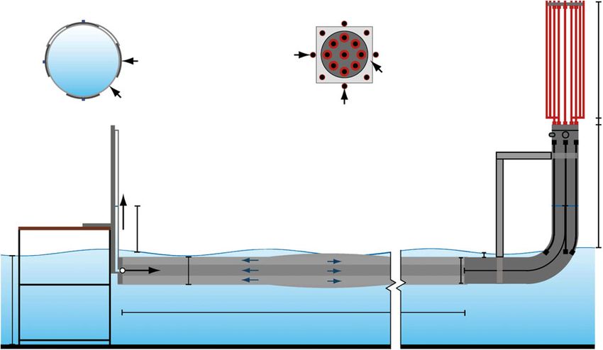
Downloaded from http://rsta.royalsocietypublishing.org/ on March 2, 2015

404                                     J. R. Chaplin et al.

filled, retaining some air above the internal liquid. Some full-scale tests and
theoretical studies were carried out in the 1950s, and were reported by Hawthorne
[2]. Besides addressing the issues of materials and construction, this research
concentrated on the analysis of the static shape of a floating flexible tube
that is partially filled, and of the stability of the tube under tow. Besides the
problem of snaking in forward motion, the tube was vulnerable to large pressures
developed by longitudinal surging of the internal liquid. This was not primarily
associated with the bulge waves that are of interest here, because the dracones
were constructed from nylon material which was practically inextensible. Thus,
the surges were accompanied not by bulges and contractions in the tube, but
by violent longitudinal motion of the air in the upper part of its cross section.
Hawthorne set out a theory for the snaking, but did not present any analysis of
internal surges. A linear numerical solution of the problem of motion of a dracone
towed in head waves is described by Zhao & Triantafyllou [3]; the theory included
longitudinal bending of the tube, but its skin was assumed to be inelastic in the
transverse direction, in accordance with the construction of the actual dracones.
The design of the dracone experiments [4] had to overcome some problems similar
to those faced in the present case, and tests on the Anaconda made use of
the same basic technique for measuring large strains in rubber, described in
detail in §3.
   Wave propagation in fluid-filled distensible tubes (as opposed to partially filled
inelastic tubes) has long been the subject of research (for reviews see [5–7]),
much of it in connection with modelling the cardiovascular system. Since blood
viscosity is clearly a factor, a frequent starting point for modelling the flow in
blood vessels (e.g. [8–10]) is Womersley’s solution [11] for the oscillatory motion
of a viscous fluid in a thin-walled elastic tube. In fact, many studies use simplified
approximations of Womersley’s velocity profiles, such as a Stokes layer near the
boundaries with a central uniform core, a power law, the Poiseuille profile or
even simply uniform flow [5]. The last of these is likely to provide a reasonable
approximation for the high Reynolds number flow in the Anaconda, and some
research in haemodynamics has focused on wave propagation in elastic tubes in
a related way, treating the liquid as incompressible and inviscid [12–14].
   For present purposes, a key property of an elastic-walled tube is its
distensibility D, defined by
                                           1 dS
                                      D=        ,                               (1.1)
                                           S dp
where S is its internal area and p the pressure difference across the tube wall
(assuming that any changes take place slowly). In the ‘linear long wavelength’
(LLW) theory, which can be traced back to Young [15], the wavelength is assumed
to be much greater than the diameter, and the material of the tube wall is
assumed to be loss-free. Convective accelerations are neglected. Wave propagation
is controlled solely by distensibility and the longitudinal inertia of the contained
liquid. In the LLW theory, waves are non-dispersive and undamped and travel at
a speed c given by [16]
                                     c = (rD)−1/2 ,                             (1.2)
where r is the fluid density. (In the biology literature, equation (1.2) is known
as the Moens–Korteweg formula.) When the conditions of the LLW theory are
not met, bulges undergo a change in shape, becoming broader and weaker as

Phil. Trans. R. Soc. A (2012)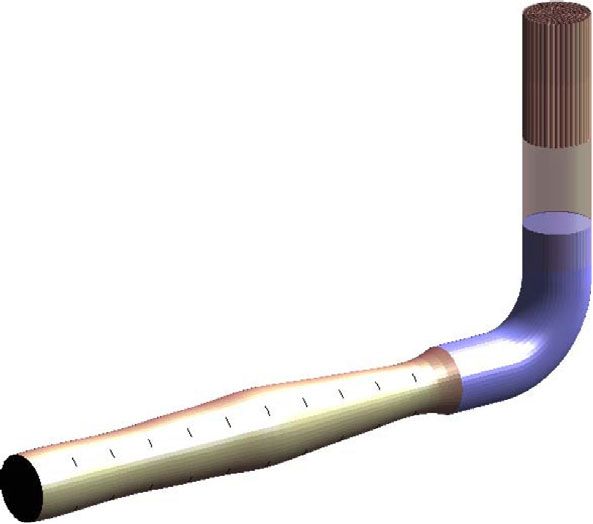
Downloaded from http://rsta.royalsocietypublishing.org/ on March 2, 2015

                                 Laboratory testing the Anaconda                           405

they advance (e.g. [17,18]). Investigating this process analytically for inviscid
incompressible fluid in a thin-walled tube, Moodie et al. [13] concluded that the
next most important effects, in order after distensibility and fluid inertia, would
be losses in the tube wall, radial inertia of fluid and wall, and bending stiffness
and rotary inertia of the wall. Just the first of these accounted for a large part
of the observed transformation. In the case of the Anaconda, other factors enter
the problem, namely inextensible sectors in the tube’s circumference, longitudinal
tension in the tube walls and the inertia of water surrounding the tube.
   The aim of the work described in this paper was to improve our understanding
of the generation and propagation of bulge waves in the Anaconda at model scale,
and to compare measured power capture with the predictions of a simple one-
dimensional theory. It was not our aim to optimize the performance of the device
or to attempt to show that it may be capable of operating on an industrial scale.
The one-dimensional theory, described in §2, extends the LLW theory to the case
of a tube of finite length and non-zero hysteresis, closed at one end and with a
PTO at the other. It neglects the effects of surface wave diffraction and radiation.
Section 3 outlines arrangements for the experiments, the results of which are
presented and discussed in §§4 and 5. Many features of the measurements are
found to be in remarkable agreement with predictions.

                                   2. Theoretical background

This section outlines some theory on various aspects of the problem, with the
aim of providing a useful background for discussion of the measurements.

        (a) Distensibility of a tube with inextensible circumferential sectors,
                                     axially restrained
   Let R0 be the radius of the unstressed tube and h0 the corresponding wall
thickness. In the experiments, the tube was made of rubber but, in order to
postpone the onset of aneurysm (see [1]), part of its circumference was covered in
longitudinal fabric strips glued to the external surface. The fabric was virtually
inextensible. Therefore, when the tube was pressurized, all of the circumferential
expansion took place in the sectors of uncovered rubber, accounting for a
proportion initially a of the total circumference.
   Suppose that, when the internal pressure exceeds the external pressure by p,
the tube has a radius of say R and a wall thickness of say h. The hoop strain
in the rubber is then 3h = (R − R0 )/aR0 . The pressure difference across the wall
is balanced by the product of the hoop tension per unit length in the uncovered
rubber sh h, where sh is the true hoop stress and the curvature of the wall 1/R,
thus sh = pR/h. If the ends of the tube are held in place (as in the experiment) and
it does not move longitudinally (or, in the language of the biological literature, is
tethered), then the rubber is in a state of plane strain, and sh = E3h /(1 − n2 ). (The
stress in the rubber in the radial direction is much smaller than sh .) This, together
with the assumptions [19] that rubber, being incompressible, has a Poisson’s ratio
n = 1/2, and that E is true stress divided by strain, leads to
                                          4Eh0       r − 1
                                     p=                         ,                         (2.1)
                                          3R0 r  (r  − 1 + a)

Phil. Trans. R. Soc. A (2012)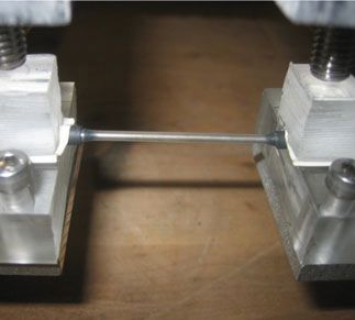
Downloaded from http://rsta.royalsocietypublishing.org/ on March 2, 2015

406                                                                 J. R. Chaplin et al.

                                                              1.1

                                free bulge wave speed ratio
                                                              1.0

                                                              0.9

                                                                0               0.5             1.0
                                                                                kR

Figure 1. Relative changes in free bulge wave speed owing to the reduction in distensibility caused
by longitudinal curvature in bulges (solid line), and owing to the presence of surrounding water
(dashed line) a = 0.45.

where r  = R/R0 . The corresponding distensibility is
                                                                     3R0 r  (r  − 1 + a)2
                                                               D=                           .         (2.2)
                                                                     2Eh0 a − (r  − 1)2
The pressure at which an aneurysm would appear (when dp/dR = 0) is
                                                                          4Eh0     1
                                                                pcrit =                    ,          (2.3)
                                                                          3R0 (1 + a1/2 )2
at a radius of R0 (1 + a1/2 ). If the pressure p were zero, and the tube were
constructed entirely of rubber (a = 1), the distensibility would be 3R0 /2Eh0 . This
is 25 per cent less than the result obtained by Lighthill [16] because here it is
assumed that the tube is constrained longitudinally.
   When bulges travel along a tube in axial tension, there is a reduction
in distensibility caused by longitudinal curvature. Suppose the radius of the
pressurized tube is R = R1 + a cos kx, where x is measured along its length, and
R1 > R0 . There is then an additional radial force per unit area in the tube,
balancing an increment in the pressure drop across the wall. This is equal to the
product of the longitudinal tension per unit circumferential length sx h (where
sx is the longitudinal stress) and the longitudinal curvature k 2 a. Proceeding as
before, with sx = nsh = sh /2 (as in plane strain), the modified distensibility D  is
given by
                                 1     1    1

                                     = + k 2 R12 p.                             (2.4)
                                D     D 4
The resulting relative increase in free bulge wave speed (D/D  )1/2 is plotted as
a function of kR in figure 1 for a = 0.45 for a tube having an internal pressure
of 75 per cent of pcrit (R1 /R0 = 1.219).
   For the experimental conditions described below (a tube of about 7 m long
and 0.25 m in diameter), the increase in free bulge wave speed would be about
3.3 per cent, 0.21 per cent and 0.05 per cent for bulge wavelengths of 1 m,

Phil. Trans. R. Soc. A (2012)
Downloaded from http://rsta.royalsocietypublishing.org/ on March 2, 2015
Laboratory testing the Anaconda 407
4 m and 8 m, respectively. Since typical wavelengths in the experiments were
towards the upper end of this range, the effect is neglected for present purposes,
though it might be significant for short bulge waves with high longitudinal
wall tension.
(b) The influence of the surrounding water on free bulge wave speed
Bulging motion in a submerged tube generates time-varying external pressures
owing to the inertia of the surrounding water. These modify the effective
distensibility and free bulge wave speed.
Consider an infinitely long deeply submerged tube of radius R conveying
regular small amplitude bulge waves of angular frequency u and wavenumber k.
The external flow generated by the passing bulges is equivalent to the effect of a
continuous travelling source distributed along the centreline of the tube, which is
taken to be the x-axis. If the source strength per unit length at x is the real part
of Aei(kx −ut) , then the total potential at an arbitrary point in cylindrical polar
coordinates (x, r) is the real part of
∞
ei(kx −ut)
f=A dx = 2AK0 (kr)ei(kx −ut) , (2.5)
−∞ (x − x ) + r
2 2
where Kn is the modified Bessel function of the second kind of order n.
In developing the theory, it is helpful to extract the time-dependence, so a
physical quantity p(x, t) is to be understood as being represented by the real
part of P(x)e−iut , where P(x) is a complex amplitude.
On the mean surface of the tube r = R, the external pressure is Pe (x)e−iut =
−r(vf/vt)r=R . The internal pressure exceeds this by the bulge pressure
Pb (x)e−iut , which is related to the tube’s area S by the distensibility,
v −iut vS vf
DS Pb (x)e = or − iuDSPb (x) = 2pR . (2.6)
vt vt vr r=R
Substituting both pressures into the bulge wave equation for zero hysteresis [1],
1 v
−u2 Pb = (Pe + Pb ), (2.7)
rD vx 2
leads to the following result for the free bulge wave speed:
u 1 2K1 (kR)
=√ . (2.8)
k rD 2K1 (kR) + kRK0 (kR)
The reduction in bulge wave speed caused by the presence of surrounding water
is plotted in figure 1. For present purposes, this is also a small effect.
(c) Bulge wave propagation with a basic power take-off and no hysteresis
It is useful to formulate a one-dimensional model for the propagation of bulge
waves in the Anaconda. The fundamentals are set out in Farley et al. [1],
but here the boundary conditions are slightly different. It is assumed that the
tube is submerged at a fixed elevation beneath regular water waves of angular
frequency u and wavenumber kw . The tube is closed and stationary at the
Phil. Trans. R. Soc. A (2012)Downloaded from http://rsta.royalsocietypublishing.org/ on March 2, 2015
408 J. R. Chaplin et al.
up-wave end (or bow), x = 0, and there is a linear dashpot PTO at the stern,
x = L. In this one-dimensional theory, diffraction and radiation of water waves
are omitted.
The tube experiences an external pressure whose complex amplitude is Pe (x) =
rgAeikw x . The bulge pressure and the internal particle velocity (assumed uniform
over the cross section) are similarly represented by their complex amplitudes
Pb (x) and
i d
U (x) = − (Pe + Pb ). (2.9)
ru dx
A solution of the wave equation (2.7) is required, with boundary conditions
U = 0 at x = 0 and U = (Pe + Pb )/rc at x = L. The latter represents a PTO that
matches the tube’s impedance, rc/S .
The solution is
i(kb +kw )L
Pb kw2 k k
w b k b e kb ei(kb +kw )L −ikb x
= 2 eikw x
− + eikb x
− e , (2.10)
rgA kb − kw2 kb2 − kw2 2(kb + kw ) 2(kb + kw )
where kb = u/c is the wavenumber of free bulge waves. The first three terms on
the right-hand side represent waves travelling in the positive x direction, the first
(hereafter denoted pw+ ) with the water wave speed u/kw , and the second and third
together (pb+ ) with the free bulge wave speed c. The fourth term (pb− ) is also a
wave with speed c, but travelling in the opposite direction.
The third and fourth terms represent a standing wave, so an alternative
formulation of equation (2.10) is
Pb kw kb ei(kb +kw )L
= 2 [k w eikw x
− k b e ikb x
] − cos kb x. (2.11)
rgA kb − kw2 kb + k w
At x = 0,
Pe + Pb kb
= [1 − ei(kb +kw )L ], (2.12)
rgA kb + k w
indicating that the total internal pressure is zero at the bow when
(kw + kb )L = 2np (2.13)
and n is an integer.
At resonance, kb = kw = k, the total internal pressure is
Pe + P b 1 1
= (2 − e2ikL − 2ikx)eikx − e2ikL e−ikx
rgA 4 4
1
= [(1 − ikx)eikx − e2ikL cos kx]. (2.14)
2
From the second of equations (2.14), it can be seen that the travelling wave (which
satisfies the bow boundary condition) has an initial amplitude equal to one-half
of that of the external wave, and a component in quadrature with the external
wave that grows linearly with x. When kx 1, it leads the external wave by 90◦ .
It also follows from equation (2.14) that if L = np/k, i.e. if the tube’s length is
an integer number of half wavelengths, the amplitude of the total internal pressure
at the stern is np/2 times that of the external pressure.
Phil. Trans. R. Soc. A (2012)Downloaded from http://rsta.royalsocietypublishing.org/ on March 2, 2015
Laboratory testing the Anaconda 409
(a) 6 +
pw
+
4 pb
|p|/rgA
–
pb
2 +
pe
0 ÂpPTO
(b) 15
P/(1/2)rgA2wS
10
5
0 0.5 1.0 1.5 2.0
w/w0
Figure 2. (a) Amplitudes of pressure in separate bulge wave components, as functions of normalized
frequency. Superscripts + and − indicate the direction of travel. Subscripts denote the wave speed:
w for the water wave, b for the free bulge wave. Thick line shows the pressure amplitude at the
PTO. (b) Power converted in the PTO with an impedance that matches the tube. The length of
the tube matches the water wavelength when u = u0 .
The mean power converted in the PTO, P = (1/2)S |Pe + Pb ||U | at x = L,
normalized with respect to the mean power that would be propagated in the
undisturbed flow across the tube’s frontal area, is
P 1
2
= [1 − cos(2kL) + 2kL sin(2kL) + 2k 2 L2 ], (2.15)
(1/2)rgA uS 8
at resonance (assuming that the water waves are in deep water). Furthermore, if
L = np/k,
P n 2 p2
= , (2.16)
(1/2)rgA2 uS 4
so that, if the tube is one wavelength long, the power gain is about 10. The
capture width derived from equation (2.16) is n 2 p2 kS/4.
It is interesting to note that the maximum power at the PTO occurs not
when kw = kb , but at a slightly higher water wave frequency: kw > kb . In deep
water conditions, kw = u2 /g and kb = uu0 /g, where u0 = g/c is the frequency at
which kb = kw . In figure 2a (in which the length of the tube is one wavelength at
u/u0 = 1), the amplitudes of the four components of the internal pressure, namely
pw+ , pb+ , pb− and the external pressure pe+ are plotted as functions of the frequency
ratio u/u0 . The first two of these approach very large values as u/u0 → 1, but
they are in anti-phase. And since these functions are not symmetrical about
u/u0 = 1, the amplitude of the total normalized pressure at the PTO (shown
as a heavy line, crossing p at u/u0 = 1), and the normalized power (figure 2b,
crossing p2 at u/u0 = 1), reach maxima elsewhere, in this case at frequencies close
Phil. Trans. R. Soc. A (2012)Downloaded from http://rsta.royalsocietypublishing.org/ on March 2, 2015
410 J. R. Chaplin et al.
(a) 4
2
p/rgA
0
–2
–4
(b) 4
2
p/rgA
0
–2
–4
0 0.5 1.0
x/L
Figure 3. Theoretical pressures over the length of the tube at 16 instants over one period;
(a) u/u0 = 1; (b) u/u0 = 1.11, at which the PTO power is maximum.
to u/u0 = 1.11. The computed progression of bulge waves is shown in figure 3,
illustrating zero pressure at the bow for u/u0 = 1 (figure 3a), and higher PTO
pressures for u/u0 = 1.11 (figure 3b).
(d) Bulge wave propagation in the conditions of the experimental set-up
Features of the experiments that can be included in a one-dimensional
theoretical approach include finite hysteresis in the rubber wall of the tube, the
presence of a slug of water between the end of the tube and the PTO, and non-
matching PTO impedance. These issues are dealt with briefly here within the
same theoretical framework, again neglecting the effect of wave diffraction and
radiation.
As mentioned below in a description of the experiment, the oscillating flow at
the end of the tube forced air back and forth through a large number of parallel
capillary pipes, which provided a linear PTO of predictable and (by closing off
some of the pipes) adjustable impedance. The layout is sketched in figure 4. The
boundary conditions are U = 0 at x = 0 as before, and
kb u 2 Pb + Pe
Z + iA 1− W U= at x = L, (2.17)
K u0 (r/D)1/2
where the impedance of the PTO is now Z rc/S , the length of the water slug
is W /K with K = u02 /g, and A is the ratio of the area of the tube to that of
the water slug. If Z = 1, the PTO matches the tube impedance, and if W = 1,
the natural frequency of the water slug is u0 .
Phil. Trans. R. Soc. A (2012)Downloaded from http://rsta.royalsocietypublishing.org/ on March 2, 2015
Laboratory testing the Anaconda 411
parallel capillary
tubes
air
slug of water of
length w in a rigid
submerged tube
bulge tube
Figure 4. Elements of the experimental arrangement. (Online version in colour.)
The effect of hysteresis in the rubber is represented by an extra term on the
right-hand side of the first of equations (2.6), which becomes
v vS v2 S
DS Pb (x)e−iut = + b 2 , (2.18)
vt vt vt
where
3 r −1+a
b = b (2.19)
4 a − (r − 1)2
and tan−1 bu = d is the loss angle [1]. The fact that losses occur only in the rubber
fraction of the circumference (which increases from its initial value a as the tube
expands), and that the rubber is assumed to be in a state of plane strain, accounts
for the term in square brackets in equation (2.19). For small loss angles, the wave
equation becomes
d 2 Pb d2 Pw
+ ru 2
D(1 + ib u)P b = − . (2.20)
dx 2 dx 2
The solution of equation (2.20) subject to the above boundary conditions reveals
the three bulge wave components mentioned earlier. The bulge wave speed is
reduced by the effect of hysteresis to become
u 1 1
=√ . (2.21)
kb rD 1
(1 + sec d)
2
The effects of mismatches between the impedances of the tube and the PTO, and
between the resonant frequencies of the tube and the water slug, are shown in
figure 5, where the normalized power is plotted as in figure 2b as a function of the
frequency ratio. In this case, the effective loss angle tan−1 b u is 10◦ . In neither
case is there a large change in the peak converted power.
Phil. Trans. R. Soc. A (2012)Downloaded from http://rsta.royalsocietypublishing.org/ on March 2, 2015
412 J. R. Chaplin et al.
(a) 8
P/(1/2)rgA2wS
W = 1.0
Z = 1.4
4
Z = 1.0
Z = 0.6
0
(b) 8
Z = 1.0
P/(1/2)rgA2wS
W = 1.4
4 W = 1.0
W = 0.6
0 0.5 1.0 1.5 2.0
w/w0
Figure 5. (a) Theoretical converted power for various PTO impedances Z and (b) for various slug
lengths W . The effective loss angle is 10◦ . The length of the tube matches the water wavelength
when u = u0 .
3. Experimental arrangements
(a) Basic set-up
These experiments were carried out in the towing tank at Southampton Solent
University. The tank is 60 m long, 3.7 m wide, with a water depth of 1.87 m. The
set-up is sketched in figure 6. The model Anaconda consisted of a 6.815 m long
rubber tube of initial diameter 0.215 m, closed at the bow, and connected to a
PTO system at the stern. In still water, the top of the tube was 40 mm below the
water surface. The apparatus was mounted on the centreline of the tank, with
the coordinate origin about 28 m from the wavemaker (a flap hinged at about
mid-depth) and 27 m from the toe of the beach.
The tube was constructed from 1 mm thick rubber sheet. As mentioned earlier,
four inelastic fabric strips were glued longitudinally to the external surface of the
tube to delay the onset of aneurysm. Placed symmetrically, they covered 55 per
cent of its circumference.
The requirements for the PTO were that it should behave like a linear dashpot,
whose impedance could be adjusted over a range that bracketed that of the tube
itself, while maintaining a positive internal pressure. Figure 6 shows a sketch of
the actual system, which came very close to achieving these aims. At the stern,
the rubber tube was connected to a stiff circular aluminium duct which turned
upwards through a swept bend. The system was filled until the water surface
inside the duct was 350 mm above the external free surface, providing the desired
operating excess pressure in the rubber tube.
Above the internal water surface, the aluminium duct terminated with
connections to 17 parallel 1 m long and 28 mm diameter copper pipes, open at
their upper ends to the atmosphere. Each copper pipe was filled with about 140
Phil. Trans. R. Soc. A (2012)Downloaded from http://rsta.royalsocietypublishing.org/ on March 2, 2015
Laboratory testing the Anaconda 413
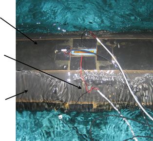
tube cross section at x = 0.545 m cross section power take-off power take-off
G1
copper pipes
G11
17 copper pipes,
1m
fabric strip ID = 0.0262 m
top plate
rubber
0.10 m
2400 tubes, ID = 0.0016 m,
length = 0.800 m
pressure reading 2 pressure transducers
hold in position
3 wave probes
1.02 m
z
0.350 m
0.04 m
x m
0.266 m 0.250 m 04
aluminium 1.
1.87 m
disc with pressure transducer bulge wave rubber tube
6.815 m
frame
Figure 6. Experimental arrangement. (Online version in colour.)
parallel stainless steel pipes of internal diameter 1.6 mm and length 800 mm. The
reversing flow in the rubber tube that accompanied the arrival of successive bulges
at the PTO caused the slug of water inside the aluminium duct to oscillate, driving
air backwards and forwards through the stainless steel pipes. The Reynolds
number of this pipe flow, a few hundred, was well within the laminar regime.
Other losses in the system were very much smaller, so the impedance of the
PTO was essentially independent of both frequency and amplitude, and could
be predicted with some confidence. It could be set between 37 and 481 kPa m−3 s
(0.64 < Z < 8.3) by closing off a number of copper pipes.
The length of the slug of water was 1.04 m. This is about 40 per cent less than
that which would correspond to a natural frequency of u0 = 2.60 rads s−1 , i.e.
W ≈ 0.6. However, according to the one-dimensional theory (figure 5), this is not
likely to result in a large change in peak converted power.
Instrumentation included resistive wave gauges at several locations in the
tank. The incident waves were monitored throughout the experiments, and
checked later in the absence of all other apparatus. A pressure transducer was
installed in the closed up-wave end of the tube. Other pressure transducers
were fitted in the PTO between the internal water surface, whose elevation was
recorded continuously with water surface elevation gauges, and the small-bore
stainless steel pipes, as shown in figure 6. Data from these transducers provided
both the impedance of the PTO and the power captured.
To measure circumferential strains in the rubber tube, we used gauges based
on the liquid metal strain gauges originally developed by Whitney [20]. Those
constructed for the present tests consisted of short silicone tubes with inner
diameter 1 mm and wall thickness 0.5 mm, filled with Galinstan, a conducting
alloy of gallium, indium and tin liquid at room temperature. The ends of the
tubes were sealed with copper electrodes of 2 mm diameter, and the electrical
Phil. Trans. R. Soc. A (2012)Downloaded from http://rsta.royalsocietypublishing.org/ on March 2, 2015
414 J. R. Chaplin et al.
(a) (b)
fabric strip
Galinstan
gauge
rubber
Figure 7. (a) Galinstan strain gauge under test. (b) Tube in the water. A Galinstan gauge can be
seen bridging a section of rubber between two fabric strips. The wire gauge above it was not used
in the present tests. (Online version in colour.)
resistance between them provided a measure of longitudinal strain. Attempts at
manufacturing such gauges using a water–copper sulphate solution as electrolyte,
like those described in an investigation of the motion of dracones [2,4], were not
successful. We found that evaporation occurred, resulting in gas bubbles and loss
of electrical continuity.
The 20 Galinstan gauges at 10 cross sections along the Anaconda tube had
initial lengths of between 64 and 76 mm, and could be stretched by as much
as 100 per cent. Their resistance was about 0.6 U and their sensitivity about
0.0004 U per per cent strain. Before installation, they were statically tested and
found to be linear to within a few per cent, and dynamic tests showed their
sensitivity to be independent of frequency over the range 0.4–4 Hz. On the model
Anaconda they were aligned in the circumferential direction, spanning a section
of rubber between adjacent fabric strips. The final calibration took place with the
gauges fixed on the tube immediately before the tests, by varying the internal
pressure and measuring the tube’s circumference. Figure 7a shows a Galinstan
gauge during testing on the bench, and figure 7b shows a gauge mounted on the
tube in the tank.
(b) Tube calibrations
Preliminary tests were carried out in still water to measure the distensibility
of the tube and the speed of free bulge waves. Results of measurements of
the tube’s circumference at various internal pressures are shown in figure 8 in
the form of tube areas as a function of pressure. They are seen to be in reasonable
agreement with equation (2.1), based on Young’s modulus of 1.3 MPa, which is
consistent with the results of simple static extension tests on rubber samples.
At the operating head of 350 mm (a pressure of 3.43 kPa—indicated by an arrow
on the pressure axis in figure 8), the tube’s area was 0.055 m2 .
An estimate of the free bulge wave speed in still water was obtained from tests
in which a single bulge was generated by impulsive motion of a piston installed
inside the tube at the bow. Data from the hoop strain gauges plotted in figure 9
record the passage of the bulge along the tube, at a mean speed of 3.34 m s−1 .
In this case, the internal pressure was 3.17 kPa. The wavelength of the impulsively
generated bulge was rather short (about 2 m) but even so the effect of longitudinal
Phil. Trans. R. Soc. A (2012)Downloaded from http://rsta.royalsocietypublishing.org/ on March 2, 2015
Laboratory testing the Anaconda 415
0.07
S (m2)
0.06
0.05
2 3 4 5
p (kPa)
Figure 8. Cross-sectional areas of the tube inferred from static measurements of hoop strain at
various internal pressures. Different symbols refer to measurements made on different occasions
over the duration of the test programme. The solid line represents equation (2.1). The dashed line
indicates the gradient dS /dp that corresponds to a bulge wave speed of 3.20 m s−1 . The operating
internal pressure is indicated by an arrow on the pressure axis.
0.070
m
55
x = 1.85 m
0.
20
x=
m
0.065
1.
m
x=
x = 2.50
m
x=
m
x = .15
x = 5.10 m
x = .80
3
5 m
S (m2)
6. m
5
m
0.060
3
x = .4
x = .75
40
4
0.055
0.050
0 1 2
t (s)
Figure 9. Tube cross-sectional areas inferred from hoop strain measurements, showing the
progression of an impulsively generated bulge. The dashed line indicates the decay calculated
for a loss angle of 9◦ .
curvature in raising the bulge wave speed (figure 1) would have been less than
1 per cent. Conversely, if the tube were deeply submerged, the surrounding water
would slow the wave by about 5 per cent (equation (2.6)). As it is, the effect of
the free surface is unknown.
According to equations (2.1) and (2.2), the effect of raising the internal
pressure from 3.17 kPa (at which the measurement of wave speed was carried
out) to the operating pressure of 3.43 kPa would be to reduce the wave speed
from 3.34 to 3.20 m s−1 . The distensibility that corresponds to 3.20 m s−1 is seen
(figure 8) to match the static measurements reasonably well, and this speed was
Phil. Trans. R. Soc. A (2012)Downloaded from http://rsta.royalsocietypublishing.org/ on March 2, 2015
416 J. R. Chaplin et al.
Table 1. PTO impedances and wave conditions.
number of wave
PTO impedance
series Z= wave periods (s) amplitudes number of tests
tube impedance
1 0.64 1.25–3.13 2 26
2 1.05 0.77–4.0 2 52
3 1.67 1.25–3.13 2 26
4 3.3 1.54–2.60 1 14
5 7.7 1.54–2.60 1 14
6 0.64–8.3 2.00 1 19
7 0.64–8.3 2.26 1 17
accordingly adopted for the purpose of identifying resonant water wave conditions
in the experiments. The corresponding tube impedance is 58.2 kPa m−3 s; with a
water depth of 1.87 m, the resonant water wave period was T0 = 2.20 s (u0 =
2.86 rads s−1 ).
The advancing bulge plotted in figure 9 lost energy to radiated waves and
hysteresis in the tube wall. The latter would cause the internal pressure to
decay as p ∼ e−gx , with g = 12 k tan d [1]. On this basis, the dashed line in figure 9
indicates the progressive reduction in area that would be associated with a loss
angle of d = 9◦ . This is in reasonable agreement with the measurements. Dynamic
tests on rubber taken from the tube wall indicated that the loss angle was about
6◦ , and it seems reasonable to assume that the additional losses in this test can
be attributed to wave radiation.
4. Experimental results and discussion
(a) Test conditions
The seven series of tests discussed below are identified in table 1. In each of the
first five series, the impedance of the PTO was kept constant and measurements
were made over a range of water wave periods T = 2p/u with wave amplitudes
a in one or two ranges. In each of the last two series, the incident wave
conditions were held constant, while the PTO impedance was varied over the
whole available range.
Some typical time series are plotted in figure 10. Figure 10a shows the
amplitudes of hoop strain increasing over the length of the tube between
Galinstan gauges G2 and G10, while figure 10b confirms that the resistance of the
PTO is in phase with the internal velocity. Since all signals were predominantly
simple harmonic, higher frequency components were neglected in the analysis
of the data.
(b) Bulge wave progression near resonance
On the assumption that cross sections of the tube remain circular, its areas
S (x, t) at the 10 gauged sections over the length of the tube were computed from
Phil. Trans. R. Soc. A (2012)Downloaded from http://rsta.royalsocietypublishing.org/ on March 2, 2015
Laboratory testing the Anaconda 417
(a) 8 G2
0
–8
hoop strain gauge extensions (mm)
8 G4
0
–8
8 G6
0
–8
8 G8
0
–8
8 G10
0
–8
48 52 56 60 64
time (s)
(b)
80
PTO air pressure (mm)
40
0
–40
–80
–80 –40 0 40 80
PTO water level (mm)
Figure 10. (a) Time series of extensions recorded by hoop strain gauges over the length of the tube
from the bow (top) to the stern. (b) Water surface elevation in the PTO is in quadrature with air
pressure. Series 2: T = 2.26 s, a = 30 mm.
the hoop strain signals. The total internal pressures p(x, t) then followed from a
finite difference solution of the wave equation [1]
v2 S S v2 p
= , (4.1)
vt 2 r vx 2
with boundary conditions provided by pressures measured at the bow and
in the PTO. Estimates of the internal velocities u(x, t) could then be found
by solving numerically the momentum equation vu/vt = −1/r(vp/vx), with
boundary conditions available from known velocities at each end. From these
computed distributions of pressures and velocities, the mean forward propagation
of power P(x) at points along the tube could be estimated.
Phil. Trans. R. Soc. A (2012)Downloaded from http://rsta.royalsocietypublishing.org/ on March 2, 2015
418 J. R. Chaplin et al.
(a) 4 measured (b) one-dimensional theory
u(x,t)/Aw 2
0
–2
–4
(c) 4 measured (d) one-dimensional theory
2
p(x,t)/rgA
0
–2
–4
0 0.5 1.0 0 0.5 1.0
x/L x/L
(e) û +/Aw :
3 measured
û+/Aw, û –/Aw
2 one-dimensional theory
û –/Aw :
1
measured
one-dimensional theory
( f)
water wave – 90°
phases (°)
360
bulge wave:
wave
measured
180 one-dimensional theory
(g) 2
P/ −²ı rga 2Cg2R
capture width (diameters)
1 measured
one-dimensional theory
0 0.5 1.0
x/L
Figure 11. Internal particle velocities (a) inferred from measurements, and (b) calculated from
one-dimensional theory, plotted over the length of the tube at 16 instants over one wave
period; (c, d) corresponding total internal pressures; (e) forward- and backward-travelling bulge
wave components, expressed in terms of corresponding particle velocity amplitudes û + and û − ;
(f ) measured and predicted phases of the forward-travelling bulge wave, plotted alongside the
water wave phase shifted by 90◦ ; (g) power in the form of capture width in diameters (Cg is the
group celerity). Series 2: T = 2.26 s, a = 30 mm, A = 29 mm.
For the case shown in figure 10, very close to resonance, figure 11 compares
several features of the measurements with predictions of the one-dimensional
theory. Internal particle velocities and total internal pressures derived from the
measurements at 16 instants over one wave period are plotted in figure 11a,c.
Phil. Trans. R. Soc. A (2012)Downloaded from http://rsta.royalsocietypublishing.org/ on March 2, 2015
Laboratory testing the Anaconda 419
2
|p|x=0 /rga
1
0
1 2 3 4 5 6
N
Figure 12. Amplitude of the internal bow pressure as a function of N = (kw + kb )L/2p.
Series 3 tests, a = 30 m.
They are normalized with respect to a representative wave particle velocity Au
and a representative pressure rgA, where, in accordance with the definition
adopted in §2, rgA is the amplitude of the pressure in the undisturbed waves
at the elevation of the centre of the tube, in this case estimated from linear
water wave theory. The lines in figure 11a,c are splines that pass through the
measurements whose locations are identified by points in other plots in figure 11.
Over the length of the tube, the maximum amplification of particle velocities
and pressures both reach about 2.8. Figure 11b,d shows corresponding particle
velocity and pressure distributions computed from the one-dimensional theory.
Similar gains are seen, though the instantaneous profiles do not match very clo-
sely. Small differences in amplitudes and phases may be enough to have this effect.
In this case close to resonance, it is reasonable to assume that the bulges travel
at the speed of the water waves, and then it becomes straightforward to separate
the forward- and backward-travelling components of the internal waves by way of
an algorithm set out in den Boer [21]. The amplitude of the internal velocity that
is associated with each wave component is plotted in figure 11e. This shows that
the forward-travelling bulge wave grows almost linearly with x, in accordance with
the particle velocity implied by the corresponding part of the first of equations
(2.14), shown as a solid line. Dashed lines represent the measured and predicted
amplitudes of the reflected waves, which are much weaker and of almost uniform
amplitude. In both cases, the measurements are in reasonable agreement with the
one-dimensional theory.
Figure 11f shows the observed phase of the forward-travelling bulge waves. It
is seen that their speed matches that of the water waves, and that they lead the
water waves by about 90◦ in accordance with equation (2.14). The corresponding
bulge wave phase obtained from equation (2.14) is shown as a solid line.
Measured and predicted power propagation is shown in the form of capture
widths in figure 11g. The last measurement point represents the power actually
converted in the PTO.
(c) Bulge wave progression in other conditions
In other conditions (not necessarily at resonance), according to the discussion
leading to equation (2.13), there should be cases in which the amplitude of the
internal bow pressure falls to zero. This is tested in figure 12, where the measured
Phil. Trans. R. Soc. A (2012)Downloaded from http://rsta.royalsocietypublishing.org/ on March 2, 2015
420 J. R. Chaplin et al.
(a) 6 (i) (ii)
360
4
|p|/rgA
q
2
180
0
(b) 6
0
4
|p|/rgA
q
2
–180
0
(c) 6 180
4
|p|/rgA
q 0
2
0 –180
(d) 12
0
8
|p|/rgA
q
4
–180
0 0.5 1.0 0 0.5 1.0
x/L x/L
Figure 13. (i) Measured amplitudes of total internal pressure and (ii) phases over the length of
the tube, plotted as points. Solid lines represent the sum of three bulge wave components with
amplitudes computed by least squares. Dashed lines represent the measured phase of the water
waves with a shift of 90◦ . (a) Series 2: T = 1.90 s, a = 26 mm; (b) series 2: T = 4.0 s, a = 46 mm;
(c) series 7: Z = 0.64, a = 30 mm; (d) series 7: Z = 3.4, a = 30 mm.
pressure is plotted against N = (kw + kb )L/2p. Some confirmation of the theory
is provided by the fact that the pressure amplitudes are highly modulated and
exhibit minima close to integer values of N .
In general, most of the motion inside the tube can be explained as the sum of
the three components of uniform amplitudes identified in the one-dimensional
theory; namely, bulge waves travelling forwards with speeds u/kw and u/kb ,
and another going in the opposite direction
at u/kb (equation (2.10)). Their
respective pressure amplitudes Pw+ , Pb+ and Pb− were estimated from the
inferred pressures in the tube by a least-squares method. Data in figure 13 support
this approach, showing that, over a wide range of conditions, amplitudes |P| and
Phil. Trans. R. Soc. A (2012)Downloaded from http://rsta.royalsocietypublishing.org/ on March 2, 2015
Laboratory testing the Anaconda 421
103
102
|p b–|/rgA
|p+w|/rgA
|p+b|/rgA
10
1
10–1
0 0.5 1.0 1.5 2.0 0 0.5 1.0 1.5 2.0 0 0.5 1.0 1.5 2.0
T/T0 T/T0 T/T0
Figure 14. Amplitudes of the three constituent bulge waves in series 2 tests plotted as functions
of relative wave period. Symbols represent the amplitudes obtained from pressures inferred from
measurements; lines show the amplitudes of the same component waves obtained from equation
(2.10) for the experimental conditions.
phases q of measured pressures at all points within the tube are in reasonable
agreement with those obtained by combining the three pressure waves.
A more severe test is to compare the pressure amplitudes of the three
constituent waves with those computed directly from the one-dimensional theory
for the same conditions. These results are plotted in figure 14 for all tests in
series 2. The pressures are normalized with respect to rgA, which in the case
of the measurements is the estimated pressure amplitude at the elevation of
the centre of the tube in the undisturbed waves. There are strong similarities,
though quantitative agreement between experimental and predicted data is not
very good, and, as in figure 11, the pressures based on measurements are generally
higher than the predictions.
(d) Power capture
Setting the impedance of the PTO higher than that of the tube results in high
pressures in the PTO, and low amplitudes of motion. If the impedance is low, the
reverse is true. At a given wave frequency, the condition for maximum converted
power is likely to be when the impedance of the PTO matches that of the tube.
In this condition, if the device had a simple dashpot PTO, were in deep water
and tuned to the wave frequency, the free bulge wave speed would be cb = g/u and
the impedance rcb /S = rg/uS . Then the relationship between pressure pPTO and
velocity uPTO in the PTO would be pPTO = (rg/uS )uPTO S , and the amplitude of
the motion in the PTO would be the same as the amplitude of the pressure head:
aPTO = uPTO /u = pPTO /rg.
This exchange between PTO pressure and displacement is illustrated in
figure 15 over a range of impedances at two wave frequencies. The points show
measurements, and the lines are computed from the one-dimensional theory
outlined in §2d. As expected, the intersection occurs close to Z = 1. The
measurements are in close agreement with the theoretical data calculated for
a loss angle of 9◦ , which also provided a good prediction for the decay of free
bulge waves in still water (figure 9), probably representing losses owing to both
hysteresis and wave radiation.
Phil. Trans. R. Soc. A (2012)Downloaded from http://rsta.royalsocietypublishing.org/ on March 2, 2015
422 J. R. Chaplin et al.
(a) (b) 5.0
5.0
|pPTO|/rgA |pPTO|/rgA
aPTO/A, |pPTO|/rgA
2.0
2.0
aPTO/A aPTO/A
1.0
1.0
0.5 0.5
0.5 1.0 2.0 5.0 10 0.5 1.0 2.0 5.0 10
Z Z
Figure 15. Points show measured (filled circles and open circles) pressures and amplitudes of motion
in the PTO from tests in (a) series 6 (T /T0 = 0.91) and (b) series 7 (T /T0 = 1.03) as functions
of PTO impedance. At Z = 1, the PTO impedance matches the tube impedance. Lines represent
results computed from the one-dimensional theory, §2d: d = 9◦ .
(a) (b)
2
capture width (diameters)
1
0
(c) 2 (d)
capture width (diameters)
1
0
0.5 1.0 1.5 0.5 1.0 1.5
T/T0 T/T0
Figure 16. Capture widths as functions of relative wave period for (a) Z = 0.64, (b) Z = 1.05,
(c) Z = 3.3, (d) Z = 7.7. Measurements are shown as points; one-dimensional theory with d = 9◦
as solid lines.
Capture widths for four different PTO impedances are plotted in figure 16 as
functions of relative wave period. The measurements are in reasonable agreement
with the theoretical results, computed with d = 9◦ . The peak power seems not
to be much affected by the PTO impedance for Z < 3.3, but the power curve
Phil. Trans. R. Soc. A (2012)Downloaded from http://rsta.royalsocietypublishing.org/ on March 2, 2015
Laboratory testing the Anaconda 423
becomes narrower as the impedance is increased. At the higher impedances, the
power peaks at wave periods below that corresponding to resonance as expected,
but there is not much evidence of this at the lowest impedances.
5. Conclusions
Experiments have been carried out on a model of the Anaconda wave energy
converter at a scale of about 1 : 25 in regular waves. The device consists of
a distensible tube in which wave energy is captured in the form of internal
oscillating flow. The model was equipped with a linear PTO of adjustable
impedance. Measurements of the distensibility of the tube and of the speed of
free bulge waves in the tube in still water agreed closely with predictions based
on known material properties.
During tests in waves, liquid metal strain gauges provided recordings of hoop
strain at 10 sections along the length of the tube, from which internal velocities,
pressures and the propagation of power were estimated. Peak capture widths were
less than two diameters, but the test conditions were not necessarily optimized
to achieve maximum power conversion.
Many features of the measurements were in surprisingly good agreement
with the predictions of a one-dimensional model for the Anaconda, based on
the assumptions that the tube remains straight and horizontal, and that the
effects of water wave diffraction and radiation can be neglected. However,
development of the theory did involve some issues that do not arise in the
analysis of wave propagation in distensible tubes in other contexts, e.g. the effects
of inelastic sectors of the circumference, longitudinal tension and the presence
of the surrounding water.
According to the theory, the fluid motion in the tube can be interpreted as the
sum of three distinct bulge wave components, one travelling forwards at the water
wave speed and one travelling in each direction at the free bulge wave speed.
The backward-travelling wave is much smaller than the others. At resonance
(when the speeds of the water waves and free bulge waves match), the forward-
travelling bulge waves grow linearly with distance along the tube, leading the
water waves by 90◦ . These conclusions were strongly supported by measurements
over a wide range of frequencies and PTO impedances. Quantitative agreement
between many measured and predicted parameters, including capture widths,
was improved by adopting a slightly higher level of hysteresis in the theory than
that which could be attributed to energy losses in the tube wall. It seems likely
that this would be unnecessary in a theory which included the effects of wave
diffraction and radiation.
This work was supported by the EPSRC (grant no. EP/F030975/1). The authors also thank
Checkmate SeaEnergy for the provision of rubber tubes, and for helpful discussions.
References
1 Farley, F. J. M., Rainey, R. C. T. & Chaplin, J. R. 2012 Rubber tubes in the sea. Phil. Trans.
R. Soc. A 370, 381–402. (doi:10.1098/rsta.2011.0193)
2 Hawthorne, W. R. 1961 The early development of the dracone flexible barge. Proc. Inst. Mech.
Eng. 175, 52–83. (doi:10.1243/PIME_PROC_1961_175_011_02)
Phil. Trans. R. Soc. A (2012)Downloaded from http://rsta.royalsocietypublishing.org/ on March 2, 2015 424 J. R. Chaplin et al. 3 Zhao, R. & Triantafyllou, M. 1994 Hydroelastic analyses of a long flexible tube in waves. In Hydroelasticity in marine technology (eds O. Faltinsen, C. M. Larsen & T. Moan), pp. 287–300. Trondheim, Norway: Balkema. 4 Fish, D. C. E. 1965 Strain measurement on the dracone flexible barge. Strain 1, 14–20. (doi:10.1111/j.1475-1305.1965.tb00048.x) 5 van de Vosse, F. N. & Stergiopulos, N. 2011 Pulse wave propagation in the arterial tree. Annu. Rev. Fluid Mech. 43, 467–499. (doi:10.1146/annurev-fluid-122109-160730) 6 Graff, K. F. 1975 Wave motion in elastic solids. Oxford, UK: Clarendon Press. 7 Pedley, T. J. 1980 The fluid mechanics of large blood vessels. Cambridge, MA: Cambridge University Press. 8 Gerrard, J. H. 1985 An experimental test of the theory of waves in fluid-filled deformable tubes. J. Fluid Mech. 156, 321–347. (doi:10.1017/S0022112085002129) 9 Horsten, J. B. A. M., Vansteenhoven, A. A. & Vandongen, M. E. H. 1989 Linear propagation of pulsatile waves in viscoelastic tubes. J. Biomech. 22, 477–484. (doi:10.1016/ 0021-9290(89)90208-X) 10 Li, J. K., Melbin, J., Riffle, R. A. & Noordergraaf, A. 1981 Pulse-wave propagation. Circ. Res. 49, 442–452. (doi:10.1161/01.RES.49.2.442) 11 Womersley, J. R. 1957 Oscillatory flow in arteries: the constrained elastic tube as a model of arterial flow and pulse transmission. Phys. Med. Biol. 2, 178–187. (doi:10.1088/ 0031-9155/2/2/305) 12 Moodie, T. B. & Barclay, D. W. 1986 Wave propagation and reflection in liquid filled distensible tube systems exhibiting dissipation and dispersion. Acta Mech. 59, 139–155. (doi:10.1007/BF01181661) 13 Moodie, T. B., Barclay, D. W. & Greenwald, S. E. 1986 Impulse propagation in liquid filled distensible tubes: theory and experiment for intermediate to long wavelengths. Acta Mech. 59, 47–58. (doi:10.1007/BF01177059) 14 Moodie, T. B., Barclay, D. W., Greenwald, S. E. & Newman, D. L. 1984 Waves in fluid filled tubes: theory and experiment. Acta Mech. 54, 107–119. (doi:10.1007/BF01190600) 15 Young, T. 1808 Hydraulic investigations, subservient to an intended Croonian lecture on the motion of the blood. Phil. Trans. R. Soc. Lond. 98, 164–186. (doi:10.1098/rstl.1808.0014) 16 Lighthill, J. 1978 Waves in fluids. Cambridge, MA: Cambridge University Press. 17 Newman, D. L., Greewald, S. E. & Moodie, T. B. 1983 Reflection from elastic discontinuities. Med. Biol. Eng. Comput. 21, 697–701. (doi:10.1007/BF02464032) 18 Ursino, M., Artioli, E. & Gallerani, M. 1993 Wave-propagation with different pressure signals: an experimental-study on the latex tube. Med. Biol. Eng. Comput. 31, 363–371. (doi:10.1007/ BF02446689) 19 Turner, D. M. & Brennan, M. 1990 The multiaxial elastic behaviour of rubber. Plast. Rubber Process. Appl. 14, 183–188. 20 Whitney, R. J. 1953 The measurement of volume changes in human limbs. J. Physiol. 121, 1–27. 21 den Boer, K. 1981 Estimation of incident and reflected wave characteristics of perpendicular wave action. Research report S4341981. Delft Hydraulics Laboratory, Delft, The Netherlands. Phil. Trans. R. Soc. A (2012)
You can also read


