The role of water in host-guest interaction - arXiv.org
←
→
Page content transcription
If your browser does not render page correctly, please read the page content below
The role of water in host-guest interaction

                                                  Valerio Rizzi1,2 , Luigi Bonati2,3 , Narjes Ansari1,2 , and Michele Parrinello1,2,4,*
                                                  1 Department    of Chemistry and Applied Biosciences, ETH Zurich, 8092 Zurich,
arXiv:2006.13274v2 [physics.comp-ph] 8 Jan 2021

                                                  Switzerland
                                                  3 Department of Physics, ETH Zurich, 8092 Zurich, Switzerland
                                                  2 Facoltà di Informatica, Istituto di Scienze Computazionali, Università della Svizzera

                                                  Italiana, Via G. Buffi 13, 6900 Lugano, Switzerland
                                                  4 Italian Institute of Technology, Via Morego 30, 16163 Genova, Italy
                                                  * michele.parrinello@phys.chem.ethz.ch

                                                  January 11, 2021

                                                  Abstract
                                                       One of the main applications of atomistic computer simulations is the calculation of ligand binding free energies. The accuracy
                                                  of these calculations depends on the force field quality and on the thoroughness of configuration sampling. Sampling is an obstacle
                                                  in simulations due to the frequent appearance of kinetic bottlenecks in the free energy landscape. Very often this difficulty is
                                                  circumvented by enhanced sampling techniques. Typically, these techniques depend on the introduction of appropriate collective
                                                  variables that are meant to capture the system’s degrees of freedom. In ligand binding, water has long been known to play a key role,
                                                  but its complex behaviour has proven difficult to fully capture. In this paper we combine machine learning with physical intuition
                                                  to build a non-local and highly efficient water-describing collective variable. We use it to study a set of of host-guest systems from
                                                  the SAMPL5 challenge. We obtain highly accurate binding free energies and good agreement with experiments. The role of water
                                                  during the binding process is then analysed in some detail.

                                                  Introduction
                                                     Host-guest interactions regulate the workings of proteins and have been intensively studied [1, 2].
                                                  Atomistic simulations have been widely used [3, 4, 5, 6, 7] to calculate key parameters like ligand affinity
                                                  and residence time, and to gain a microscopic understanding of how protein-ligand binding works. The
                                                  accuracy of these simulations depends on two key aspects: the quality of the model used to describe
                                                  the interatomic interactions and the thoroughness of the statistical sampling [8, 9]. In this work we will
                                                  focus only on the latter and we will show that sampling can be much improved if the role of water in the
                                                  binding-unbinding processes is duly taken into account.
                                                     Binding processes take place on a timescale that is unreachable with current computer resources, thus
                                                  the use of enhanced sampling methods is mandatory. We will frame our discussion in the context of Meta-
                                                  dynamics (MetaD) [10, 11, 12] or, more precisely, of its most recent evolution, the on-the-fly probability-
                                                  enhanced sampling method (OPES) [13]. OPES, like MetaD and many other methods [14, 15, 16], relies
                                                  on the identification of suitable order parameters or collective variables (CVs). In these methods [14, 17],
                                                  the CV distribution is made to follow a preassigned law. This allows CVs fluctuations to be amplified in
                                                  a controlled way. For such methods to work in an accurate and efficient manner, the CVs must be able
                                                  to describe the slow degrees of freedom of the system. Here we will identify one such powerful CV of
                                                  general applicability aimed at describing the role of water in the ligand binding process.

                                                                                                                    1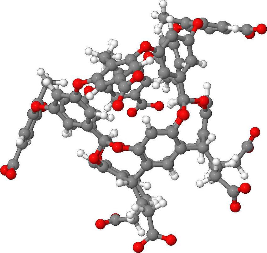
G1                             G2
                                            0        2
             z (Å)                                       r (Å)                                           L4
                                       V8                                       L4
                                                                                                                          L1
             15                        V7                                       L3       L2                   L2
                                                                                              L1
                                       V6                                                                                          L3

             10                                                      G3        L4                   G4
                                       V5                                                                          L3
                                   t
                                in
                               ra
                            st

                                       V4
                          re

                                                                          L3
                       el

                                                                                                         L1
                     nn

                                                V3                                                                       L2
                                                                                    L2
                  Fu

             5
                                                                                               L1                             L4

                                             V2                      G5                             G6
                                                                                                                    L4
             0
                                        V1                                     L4
                                                                                     L3
                                                                                                              L2
                                                                                                                              L3
                                                                                              L2
                                                                                    L1                   L1

Figure 1: Sketch of the octa-acid host OAMe with the funnel restraint geometry and the guest molecules
from the SAMPL5 challenge. We indicate the position of the points where the descriptors are centred
and hint at their spatial outreach by drawing surfaces at a constant radius around some of them.

    Water is expected to play an important role since, upon entering the binding site, the ligand has to
shed its solvation shell in toto or in part, while the water that originally was in the binding site has to
rearrange and negotiate its way out of the binding cavity. Not surprisingly much effort has been devoted
on the role of water in ligand-host binding [18, 19, 20, 21, 22, 23, 24]. In the context of enhanced sampling
many attempts have been made at capturing the role of water in a CV, leading to an improvement in
binding free energy estimations [25, 5, 26, 27, 28]. We show here that there is room for a further decisive
step as none of these water-related CVs has been able to describe accurately the highly non-local changes
in water structure that take place during binding, both in the vicinity of the ligand and in and around the
binding pocket.
    In order to succeed in our endeavour, we rely on a combination of physical considerations and modern
machine learning (ML) techniques. In particular, we use a method that we have recently developed which
goes under the name of Deep Linear Discriminant Analysis (Deep-LDA) [29]. Deep-LDA builds efficient
CVs from the equilibrium fluctuations of a large set of descriptors, expressing them as a neural network
(NN). In this context, the choice of descriptors is essential and we appeal to our physical understanding
to introduce one such set that is capable of characterising not only the ligand solvation shell but also the
water structure inside and outside the binding cavity. After building such a CV, we use it in OPES for
accelerating the sampling of binding-unbinding events.
    We measure the performance of our approach on a set of test systems taken from the SAMPL5 com-
petition [30, 31, 32] and study the interaction of six ligands with an octa-acid calixarene host (OAMe) (see
Fig. 1). We choose this system because, despite its relative simplicity, it retains most of the key features
of a biologically relevant protein-ligand system. Very recently, a closely related system has been used to
investigate how water flows in and out of the system in the absence of a ligand [33]. Furthermore, the
host’s symmetry simplifies the analysis and comparison can be made to existing theoretical calculations
[32]. The choice to perform simulations on a system with a standard set of simulation parameters allows

                                                                 2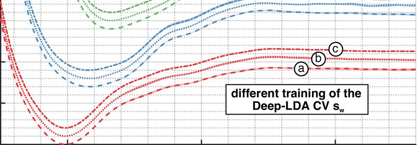
Descriptors
                           d                                  LDA Eigenvector w
                      L1
                            L2                   Hidden
                      L3                          layer
                                                    h
                            L4
                      V1
                                                                                     Deep-LDA CV
                            V2
                                                               Linear                  sw=s+s3
                      V2
                                                            combination
                            V4
                      V5                                                           s=wTh
                            V6                                                    NN output
                      V7
                            V8

Figure 2: Schematics of the Deep-LDA architecture used in this work. The descriptors d are fed to a NN
that generates s as a linear combination of the last NN hidden layer h and the LDA eigenvector w. The
Deep-LDA CV is then sw = s + s3 .

our results to be compared to a range of different techniques, among which the attach-pull-release method
[34], alchemical protocols [35] and metadynamics [36].

Results
Collective variables from equilibrium fluctuations with Deep-LDA
    In this work, we are mainly interested in computing the free energy difference ∆G between the bound
state (B) in which the ligand sits in the lowest free energy binding pose and the unbound state (U) where
the ligand is solvated in water and free to diffuse. In order to obtain a CV able to capture water behaviour
we use the recently developed machine learning Deep-LDA method [29].
    Deep-LDA is a non-linear evolution of the time-honoured Linear Discriminant Analysis (LDA) classi-
fication method [37]. In LDA, one takes two sets of data, in our case the configurations visited in short
unbiased simulations in B and U, and defines a set of Nd descriptors d that are able to distinguish between
the two. The aim of LDA is to find the linear combination of descriptors s = w T d that best separates the
two sets of data, w being a Nd -dimensional vector.
    To this effect, one calculates for each set of data the vectors of the average descriptors values µB , µU
and their variance matrices SB , SU . With these quantities, one then computes the so-called Fisher’s ratio:

                                                        w T Sb w
                                             J (w ) =            .                                        (1)
                                                        w T Sw w

where one has defined the within scatter matrix Sw = SB + SU and the between one Sb = (µB − µU ) (µB − µU ) T .
The w that maximises this ratio is the direction that optimally discriminates the two states and gives the
best separated projection of the data in the one-dimensional s space. The variable thus obtained has been
shown to perform well as CV in many cases, especially if one uses its Harmonic LDA variant [38, 39].
    In Deep-LDA, a similar paradigm applies with the key difference that LDA is performed on a non-
linear transformation of the descriptors. The non-linearity is introduced by a neural network (NN) (see
Fig. 2) whose input is the set of Nd descriptors d and the outputs are the Nh components of the last hidden
layer h. LDA is performed on the components of h, so that, after determining the corresponding Sw and
Sb , the NN is optimised using J (w ) as loss function. At convergence, one determines the weights of the
NN and the Nh -dimensional optimal vector w that produces the Deep-LDA projection:

                                                 s = w T h.                                               (2)

                                                        3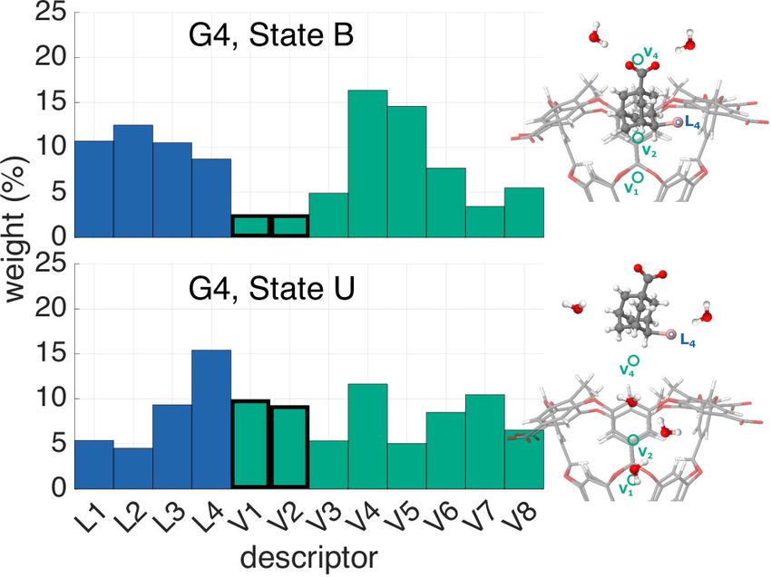
Deep-LDA is a powerful classifier that tends to compress the data into very sharp distributions which
are unsuitable for enhanced sampling applications. To address this issue, we smooth the distributions by
applying the following cubic transformation sw = s + s3 , in the spirit of what was done in Ref. [40]. The
CV thus obtained will be used to describe water behaviour in our simulations.

Including water in the model
    The choice of the descriptors d is of paramount importance since it implies the physics that we want
to describe. In our case, we are interested in capturing the role of water in the binding process. To this
effect, we choose two sets of points around which we compute the water coordination number. One set is
located on the ligand, while the second one is fixed along the host’s axis z at regular intervals (see Fig. 1
and the Supplementary Methods).
    The first set of coordination numbers {Li } describes water solvation around the ligand and is similar
in spirit to the ligand solvation variables that have been used in the past [5, 28]. The second one {Vi }
is aimed instead at capturing the water arrangement inside and outside the binding pocket without any
explicit reference to the ligand. It is essential that the descriptors capture all the water molecules that
contribute to the host and the guest solvation. Missing some of them would create a incomplete picture
of solvation, which in turn would lead to Deep-LDA classification errors and ineffective bias.
    The set of descriptors {Li , Vi } gives information on the structure of water and its non-local changes
on a small to medium length scale during the binding-unbinding process. Its effectiveness does not lie in
the individual action of each descriptor but in its collective capability to capture the many-body concerted
movements of host, guest and water molecules. The use of these descriptors is one of the elements of
novelty in our approach and one of the keys to its success.

Binding free energies from enhanced sampling simulations
    We perform OPES simulations to estimate the binding free energies of all the six ligands of Fig. 1. We
use the Deep-LDA CV sw together with a second CV sz , that is the projection of the ligand centre of mass
on the binding axis z. In the ligand binding context, using the latter is a natural choice [5, 36] as it has
a clear physical interpretation and helps distinguishing B from U. Furthermore, we employ a funnel-like
restraint potential [4] to encourage the ligand to find its way back to the binding site once it is out in
the solution. The entropic correction to the free energy due to the funnel restriction can be calculated
analytically (see Eq. 4 in the Supplementary Methods) and is taken into account when computing the
binding free energies ∆G. We refer the interested reader to the Supplementary Methods for further details.
    The combined use of these two CVs leads to an efficient sampling, which is reflected in a high number
of binding-unbinding events per unit time (see for example Supplementary Fig. 18). We notice a clear
improvement over a more standard set of CVs [36], namely sz itself and the cosine of the angle θ between
the binding axis z and the ligand orientation (see Supplementary Fig. 17). The introduction of a water-
based CV in enhanced sampling simulations allows the system to reach a regime where it diffuses without
hysteresis from one metastable state to another, yielding a high accuracy in estimating ensemble averages
of physical quantities. This makes it possible to significantly reduce the error bars without having to
increase the computational time relative to what reported in the literature [34].
    Performing enhanced sampling simulations allows retrieving the equilibrium distribution P(s) of
any collective variable s [14]. Here we focus on the free energy surface (FES), defined as FES(s) =
−kB T log P(s) where kB is the Boltzmann constant and T is the temperature of the system. In the context
of ligand binding, it is customary to look at the FES as a function of the host-guest distance sz . For each
of the six ligands we compute the FES and estimate the errors with a block average analysis. We report
these results in Fig. 3 in which we also assess the robustness of the Deep-LDA CV by showing the results
corresponding to three different Deep-LDA training.
    We then report the binding free energies ∆G corrected for the presence of the funnel in Tab. 1. In
Fig. 4 we compare them with experimental values and theoretical calculations performed on the same
model but with different sampling techniques [35, 34, 36]. We assess the quality of our estimates through
the metrics used in the SAMPL5 overview paper [32] and obtain a root mean-squared error of 0.68 kcal

                                                     4
45
                                                                                      G6

                                          40
                                                                                      G5
                                          35

                       FES (kcal mol-1)
                                          30
                                                                                      G4
                                          25                                          G3

                                          20
                                                                                      G2
                                          15

                                          10                                          G1

                                           5

                                           0
                                               5               10                15
                                                              s z (Å)

Figure 3: Free energy surfaces projected along the host-guest distance. For each of the six ligands, we
compute the free energy along the sz variable using a standard umbrella-sampling-like reweighting for-
mula to recover the unbiased distribution [13]. The shaded areas indicate the errors, whose calculation is
detailed in the Supplementary Methods. To ensure that the results do not depend on a specific realisation
of the Deep-LDA CV, we repeat the training three times by using different initial weights of the NN.
The resulting CVs are denoted as sw  a , sb and sc and the corresponding FES are indicated respectively by
                                          w      w
dashed, dotted and dash-dotted lines. For clarity, curves related to the same ligand but with different CVs
are shifted by 1 kcal mol−1 , while the shift between different ligand curves is 5 kcal mol−1 .

Table 1: Binding free energies. We show the mean binding free energy ∆G (kcal mol−1 ) for every
ligand and the corresponding experimental value. We calculate ∆G as a weighted block average over the
simulations with all Deep-LDA CVs (see the Supplementary Methods for further details).
                                                   Ligand   Deep-LDA       Exp
                                                    G1      −6.31 ± 0.06   -5.24
                                                    G2      −6.19 ± 0.08   -5.04
                                                    G3      −6.27 ± 0.07   -5.94
                                                    G4      −2.51 ± 0.07   -2.38
                                                    G5      −3.91 ± 0.09   -3.90
                                                    G6      −4.97 ± 0.07   -4.52

mol−1 , a Pearson coefficient of determination of 0.93, a linear regression slope of 1.21 and a Kendall
correlation coefficient of 0.87. With some exceptions, we are in line with the SAMPL5 results (see Fig. 4
and Supplementary Tab. 1-2). However, the error bars are significantly reduced over the whole set of
ligands investigated.
    To test the generality of our procedure, we investigate the interaction of the six ligands with the OAH
host also studied in the SAMPL5 challenge. The results are in agreement with those reported in Refs. [35,
34, 36] and in Supplementary Fig. 31-57 and Tab. 9-16 we provide a complete report. As a further check of

                                                                5
(b)
(a)
(kcal mol-1)
ΔGDeep-LDA = 1.21 ΔGexp + 0.40 kcal mol -1 G4
(kcal mol-1)
R2 = 0.93
G5
G6
G3
G2
G1
G1 G2 G3 G4 G5 G6
(kcal mol-1) ligand
Figure 4: Comparison of the binding free energies with experiments and other calculations. In (a), we
plot the value of ∆G obtained from the Deep-LDA simulations (in blue crosses) for every ligand versus
the experimental values and show the corresponding linear fit. In (b), we report their difference with
the experimental values and compare them with other computational results performed using the same
simulation setup. Results from [36] are indicated with red circles, from [34] in green diamonds and
from [35] in yellow squares.
our method and of the role of water, we also perform simulations of the host OAMe with the six ligands
using the TIP4P/EW water model [41] instead of the TIP3P model [42]. While the binding/unbinding
process is unchanged, we find that the binding free energies depend on the water model chosen. Modulo
a shift of about 1.3 kcal mol−1 , the two sets of results correlate reasonably well with one another and with
the experiments. For a quantitative assessment of this statements, see Supplementary Fig. 59-78 and Tab.
19-26. The root of this change can be possibly attributed to a different solubility of the ligand in the two
water models and to a different host-water interaction.
The case of G4
The use of the Deep-LDA CV sw not only allows us to obtain accurate binding free energies but also
a detailed insight into water behaviour during the binding process. We illustrate here the case of G4, the
guest that exhibits the most complex behaviour, and refer the interested reader to Supplementary Fig. 5-30
and Tab. 3-8 for a detailed analysis of all the other ligands.
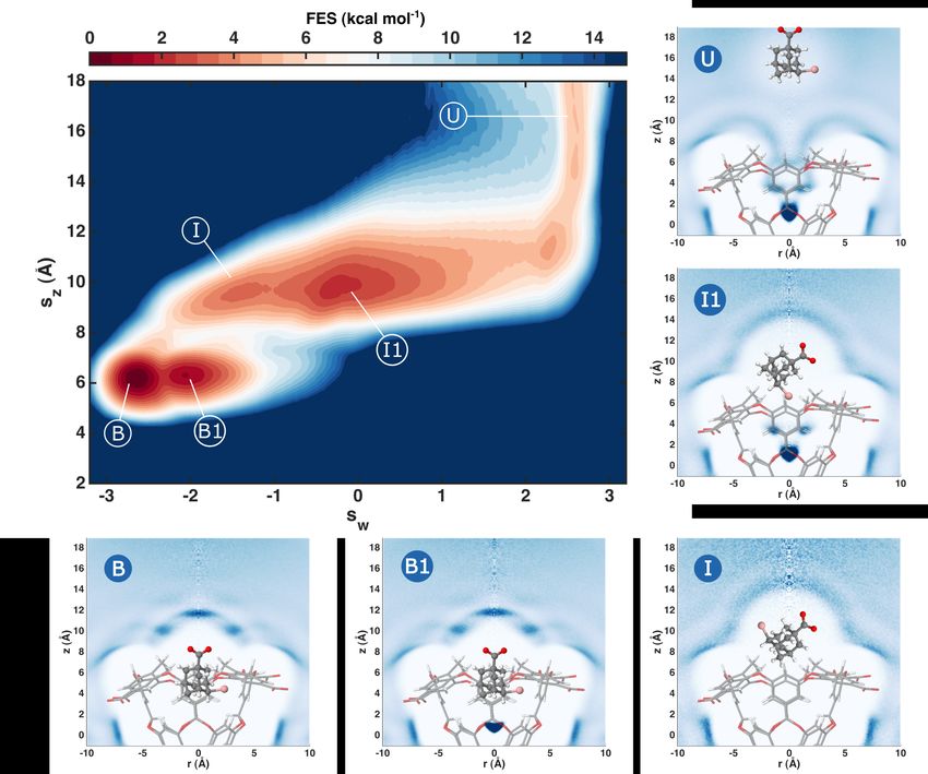
In Fig. 5 we show the FES of G4 and the cylindrically averaged water density in the metastable states.
We find that the system presents two binding poses B and B1. The lowest free energy binding pose B is
the same as the one found in the experiments and contains no water. Our simulation discovered a second
binding pose B1 that differs from B for the presence of a water molecule at the centre of the cavity. This
second pose is ≈ 2 kB T higher in free energy and thus it is occupied with a much lower probability.
When the ligand exits the pocket, before being fully solvated, it can pass through two intermediate
short lived states I and I1. In I, the cavity is dry and the ligand is free to rotate in front of the cavity
entrance. In I1, the ligand sits again in front of the host entrance but its rotation favour configurations
in which the ligand bromine atom points towards the cavity forming a linear arrangement where a water
at the centre of the cavity is bridged by another water to the Br− anion (see Supplementary Fig. 21). We
underline that neither B1 nor I and I1 were part of the Deep-LDA training.
The ability of the Deep-LDA CV sw to capture the non-local water structural changes is the main
reason behind our capability to study the system’s FES and its metastable states at this level of detail.
6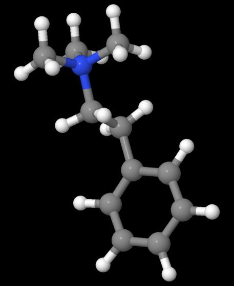
Figure 5: Binding FES of ligand G4 with a study of the water presence in the visited states. We show the
two-dimensional FES of the ligand G4 with respect to sz and Deep-LDA CV sw . Different adjacent colours
corresponds to a free energy difference of 1 kB T ≈ 0.6 kcal mol−1 . We highlight some relevant states
over which we perform plain molecular dynamics (MD) simulations to measure the presence of water.
We show histograms of the water oxygen atoms density in cylindrical coordinates z, r. Each histogram
is normalised by the density value in its top right corner and darker colours correspond to higher water
density regions. The position of the ligand in these plots is illustrative.

For instance, the use of CVs that concentrate solely on the position of the ligand with respect to the
binding site such as sz alone would clearly lead to an incomplete picture. In fact, B and B1 (and similarly
I and I1) cannot be distinguished properly by sz and, without the presence of a bias changing the cavity’s
solvation, the limiting timescale of the simulations would be the water movement in and out of the pocket.
Furthermore, local CVs that only describe the average ligand solvation can only partially take into account
these non-local effects.

                                                    7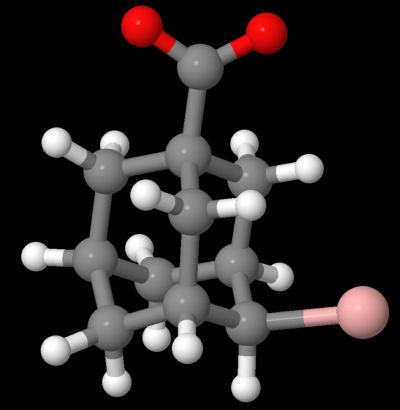
G4, State B

Figure 6: Descriptors relative weights for guest G4. Following the derivative-based ranking from
Ref. [29], we show the relative weight that each descriptor has in the Deep-LDA CV in the bound and
the unbound state of guest G4. We show the average weight over the 3 different Deep-LDA CVs that we
trained. The V1 , V2 descriptors, which measures the number of molecules inside the pocket, are outlined
to mark the significant change in their contribution between the two states.

Analysis of the role of water
    We can gain a deeper insight of the role of water by investigating the dependence of the Deep-LDA
CV on the {Li , Vi } descriptors. This can be done by analysing the descriptors’ relevance in the action of
sw and, for doing that, we use the derivative ranking method illustrated in Ref. [29]. Here, we separate
the role of the descriptors in the bound and unbound state and we report the results of ligand G4 in Fig. 6
(see Supplementary Fig. 22 for an analysis over all the G4 metastable states).
    Both in state B and U, the weights are distributed over a wide range of descriptors pointing to the
fact that the Deep-LDA CV is able to capture the complex non-local action of water. However, different
descriptors act in different ways in the two states. In the B state, the descriptors V4 , V5 that are linked to
the water molecules that reside in the proximity of the host’s entrance have more weight. This indicates
that the fluctuations in this part of the water system need to be amplified for the ligand to exit.
    In contrast, in the U state, the descriptors that gain more weight are L4 which measures the solvation
around the Bromine atom of the ligand and V1 , V2 that control the quantity of water contained in the
binding cavity. Fluctuations towards the dry state of the cavity need to occur for the ligand to bind. Such
fluctuations can occur with a small but not negligible probability also in the holo state (see Supplementary
Fig. 2). Even larger fluctuations have been observed experimentally in Ref. [33] in a related system. We
expect these fluctuations to be an important part of the reaction process in many host-guest systems.
    The non-local action of the Deep-LDA CV is thus reflected in the relevance given to different water-
based descriptors, depending on whether the system is in the bound or unbound state. When enhancing
the sampling of this CV, this non-locality determines a collective motion of water that encourages the
occurrence of binding/unbinding events.

Discussion
   We have shown that, even in the relatively simple systems studied here, a complex and subtle reor-
ganisation of water structure takes place and our strategy is able to capture it. Our calculations offer a
powerful analysis tool and lead to accurate binding free energies.
   Often, in the paper, we have underlined the efficiency of our method. However, this was not done in a
spirit of competition with the SAMPL5 participants who, by the way, did not have the benefit of knowing

                                                       8
the results beforehand. Our aim was instead to uncover and describe the role of water through the design
and the application of an effective CV. In a scheme like MetaD, the efficiency of a CV is measured by its
ability to capture the physics of the problem, hence our insistence on efficiency.
    Having been able to reduce this much the sampling error on a commonly used model, we might even
be tempted to claim that the discrepancies with respect to experiments can be blamed mainly on the
inaccuracy of the force field. It would be interesting in this respect to investigate the force field limitations
and how the inclusion of effects like polarisation could bring the results closer to experiments. The method
is very robust and defines a protocol that can be naturally applied to larger and more complex systems.
In fact, the sampling proficiency of our method will prove even more crucial in complex scenarios where
a large number of water molecules can be trapped in multiple pocket locations.

                                                       9
Data Availability
   The simulations inputs were taken from https://github.com/michellab/Sire-SAMPL5. We perform
the simulations with GROMACS 2019.4 [43] using the GAFF force field [44] with RESP charges [45]
and the TIP3P water model [42]. For enhanced sampling we use a custom version of the PLUMED
plugin 2.5.4 [46] where we include OPES [13] and the Pytorch library 1.4 [47]. More details can be
found in the Supplementary Methods. Simulations data are available on the Materials Cloud Archive at
DOI:10.24435/materialscloud:p3-1x.

Code Availability
    All the inputs and instructions to reproduce the results presented in this manuscript are deposited in
the PLUMED-NEST repository at plumID:20.025. A tutorial about the Deep-LDA training can be found
at this link.

References
 [1] Michel, J. & Essex, J. W. Prediction of protein-ligand binding affinity by free energy simulations:
     assumptions, pitfalls and expectations. Journal of Computer-Aided Molecular Design 24, 639–658 (2010).
     URL http://link.springer.com/10.1007/s10822-010-9363-3.

 [2] Mobley, D. L. & Gilson, M. K. Predicting Binding Free Energies: Frontiers and Benchmarks. An-
     nual Review of Biophysics 46, 531–558 (2017). URL http://www.annualreviews.org/doi/10.1146/
     annurev-biophys-070816-033654.
 [3] Bronowska, A. Thermodynamics of Ligand-Protein Interactions: Implications for Molecular De-
     sign. In Thermodynamics - Interaction Studies - Solids, Liquids and Gases, vol. i (InTech, 2011). URL
     http://www.intechopen.com/books/thermodynamics-interaction-studies-solids-liquids-
     and-gases/thermodynamics-of-ligand-protein-interactions-implications-for-molecular-
     design.
 [4] Limongelli, V., Bonomi, M. & Parrinello, M. Funnel metadynamics as accurate binding free-energy
     method. Proceedings of the National Academy of Sciences 110, 6358–6363 (2013). URL http://www.pnas.
     org/cgi/doi/10.1073/pnas.1303186110.
 [5] Tiwary, P., Mondal, J. & Berne, B. J. How and when does an anticancer drug leave its binding site?
     Science Advances 3, e1700014 (2017). URL https://advances.sciencemag.org/lookup/doi/10.1126/
     sciadv.1700014.
 [6] Evans, R. et al. Combining Machine Learning and Enhanced Sampling Techniques for Efficient and
     Accurate Calculation of Absolute Binding Free Energies. Journal of Chemical Theory and Computation
     16, 4641-4654 (2020). URL https://pubs.acs.org/doi/10.1021/acs.jctc.0c00075.
 [7] Limongelli, V. Ligand binding free energy and kinetics calculation in 2020. WIREs Computational
     Molecular Science 10, 1–32 (2020). URL https://onlinelibrary.wiley.com/doi/abs/10.1002/wcms.
     1455.

 [8] Mobley, D. L. Let’s get honest about sampling. Journal of Computer-Aided Molecular Design 26, 93–95
     (2012). URL http://link.springer.com/10.1007/s10822-011-9497-y.
 [9] Rizzi, A. et al. The SAMPL6 SAMPLing challenge: assessing the reliability and efficiency of binding
     free energy calculations. Journal of Computer-Aided Molecular Design 34, 601–633 (2020). URL https:
     //doi.org/10.1007/s10822-020-00290-5.

                                                    10
[10] Laio, A. & Parrinello, M. Escaping free-energy minima. Proceedings of the National Academy of Sciences
99, 12562–12566 (2002). URL http://www.pnas.org/cgi/doi/10.1073/pnas.202427399.
[11] Barducci, A., Bussi, G. & Parrinello, M. Well-Tempered Metadynamics: A Smoothly Converging and
Tunable Free-Energy Method. Physical Review Letters 100, 020603 (2008). URL https://link.aps.
org/doi/10.1103/PhysRevLett.100.020603.
[12] Bussi, G. & Laio, A. Using metadynamics to explore complex free-energy landscapes. Nature Reviews
Physics 2, 200–212 (2020). URL http://dx.doi.org/10.1038/s42254-020-0153-0.
[13] Invernizzi, M. & Parrinello, M. Rethinking Metadynamics: From Bias Potentials to Probability Distri-
butions. The Journal of Physical Chemistry Letters 11, 2731–2736 (2020). URL https://pubs.acs.org/
doi/10.1021/acs.jpclett.0c00497.
[14] Valsson, O., Tiwary, P. & Parrinello, M. Enhancing Important Fluctuations: Rare Events and Metady-
namics from a Conceptual Viewpoint. Annual Review of Physical Chemistry 67, 159–184 (2016). URL
http://www.annualreviews.org/doi/10.1146/annurev-physchem-040215-112229.
[15] Tiwary, P. & van de Walle, A. A Review of Enhanced Sampling Approaches for Accelerated Molecular
Dynamics. In Multiscale Materials Modeling for Nanomechanics, chap. 6, 195–221 (Springer, 2016). URL
http://link.springer.com/10.1007/978-3-319-33480-6_6.
[16] Debnath, J. & Parrinello, M. Gaussian Mixture-Based Enhanced Sampling for Statics and Dynamics.
The Journal of Physical Chemistry Letters 11, 5076–5080 (2020). URL https://pubs.acs.org/doi/10.
1021/acs.jpclett.0c01125.
[17] Invernizzi, M., Piaggi, P. M. & Parrinello, M. A Unified Approach to Enhanced Sampling. Preprint
at http://arxiv.org/abs/2007.03055 (2020).
[18] Ladbury, J. E. Just add water! The effect of water on the specificity of protein-ligand binding sites
and its potential application to drug design. Chemistry & Biology 3, 973–980 (1996). URL https:
//linkinghub.elsevier.com/retrieve/pii/S1074552196901647.
[19] Ewell, J., Gibb, B. C. & Rick, S. W. Water inside a hydrophobic cavitand molecule. Journal of Physical
Chemistry B 112, 10272–10279 (2008).
[20] Abel, R., Young, T., Farid, R., Berne, B. J. & Friesner, R. A. Role of the Active-Site Solvent in the
Thermodynamics of Factor Xa Ligand Binding. Journal of the American Chemical Society 130, 2817–2831
(2008). URL https://pubs.acs.org/doi/10.1021/ja0771033.
[21] Wang, L., Berne, B. J. & Friesner, R. A. Ligand binding to protein-binding pockets with wet and dry
regions. Proceedings of the National Academy of Sciences 108, 1326–1330 (2011). URL http://www.pnas.
org/cgi/doi/10.1073/pnas.1016793108.
[22] Mahmoud, A. H., Masters, M. R., Yang, Y. & Lill, M. A. Elucidating the multiple roles of hydration for
accurate protein-ligand binding prediction via deep learning. Communications Chemistry 3, 19 (2020).
URL http://dx.doi.org/10.1038/s42004-020-0261-x.
[23] Bergazin, T. D. et al. Enhancing Water Sampling of Buried Binding Sites Using Nonequilibrium
Candidate Monte Carlo. Preprint at https://doi.org/10.26434/chemrxiv.12429464 (2020).
[24] Ben-Shalom, I. Y. et al. Accounting for the Central Role of Interfacial Water in Protein-Ligand Binding
Free Energy Calculations. Preprint at https://doi.org/10.26434/chemrxiv.12668816 (2020).
[25] Limongelli, V. et al. Sampling protein motion and solvent effect during ligand binding. Proceedings of
the National Academy of Sciences of the United States of America 109, 1467–1472 (2012).
11[26] Casasnovas, R., Limongelli, V., Tiwary, P., Carloni, P. & Parrinello, M. Unbinding Kinetics of a p38
MAP Kinase Type II Inhibitor from Metadynamics Simulations. Journal of the American Chemical Society
139, 4780–4788 (2017).
[27] Brotzakis, Z. F., Limongelli, V. & Parrinello, M. Accelerating the Calculation of Protein–Ligand Bind-
ing Free Energy and Residence Times Using Dynamically Optimized Collective Variables. Journal of
Chemical Theory and Computation 15, 743–750 (2019). URL https://pubs.acs.org/doi/10.1021/acs.
jctc.8b00934.
[28] Pérez-Conesa, S., Piaggi, P. M. & Parrinello, M. A local fingerprint for hydrophobicity and hy-
drophilicity: From methane to peptides. The Journal of Chemical Physics 150, 204103 (2019). URL
http://dx.doi.org/10.1063/1.5088418.
[29] Bonati, L., Rizzi, V. & Parrinello, M. Data-Driven Collective Variables for Enhanced Sampling.
The Journal of Physical Chemistry Letters 2998–3004 (2020). URL http://dx.doi.org/10.1021/acs.
jpclett.0c00535.
[30] Bannan, C. C. et al. Blind prediction of cyclohexane–water distribution coefficients from the
SAMPL5 challenge. Journal of Computer-Aided Molecular Design 30, 927–944 (2016). URL http:
//link.springer.com/10.1007/s10822-016-9954-8.
[31] Sullivan, M. R., Sokkalingam, P., Nguyen, T., Donahue, J. P. & Gibb, B. C. Binding of carboxylate and
trimethylammonium salts to octa-acid and TEMOA deep-cavity cavitands. Journal of Computer-Aided
Molecular Design 31, 21–28 (2017).
[32] Yin, J. et al. Overview of the SAMPL5 host–guest challenge: Are we doing better? Journal of
Computer-Aided Molecular Design 31, 1–19 (2017). URL http://link.springer.com/10.1007/s10822-
016-9974-4.
[33] Barnett, J. W. et al. Spontaneous drying of non-polar deep-cavity cavitand pockets in aqueous solution.
Nature Chemistry 12, 589–594 (2020). URL http://dx.doi.org/10.1038/s41557-020-0458-8.
[34] Yin, J., Henriksen, N. M., Slochower, D. R. & Gilson, M. K. The SAMPL5 host–guest challenge:
computing binding free energies and enthalpies from explicit solvent simulations by the attach-pull-
release (APR) method. Journal of Computer-Aided Molecular Design 31, 133–145 (2017). URL http:
//link.springer.com/10.1007/s10822-016-9970-8.
[35] Bosisio, S., Mey, A. S. & Michel, J. Blinded predictions of host-guest standard free energies of binding
in the SAMPL5 challenge. Journal of Computer-Aided Molecular Design 31, 61–70 (2017).
[36] Bhakat, S. & Söderhjelm, P. Resolving the problem of trapped water in binding cavities: prediction
of host–guest binding free energies in the SAMPL5 challenge by funnel metadynamics. Journal of
Computer-Aided Molecular Design 31, 119–132 (2017).
[37] Welling, M. Fisher Linear Discriminant Analysis. Tech. Rep., Dep. Comput. Sci. Univ. Toronto (2005).
[38] Mendels, D., Piccini, G. & Parrinello, M. Collective Variables from Local Fluctuations. The Jour-
nal of Physical Chemistry Letters 9, 2776–2781 (2018). URL http://pubs.acs.org/doi/10.1021/acs.
jpclett.8b00733.
[39] Capelli, R. et al. Chasing the Full Free Energy Landscape of Neuroreceptor/Ligand Unbinding by
Metadynamics Simulations. Journal of Chemical Theory and Computation 15, 3354–3361 (2019). URL
http://pubs.acs.org/doi/10.1021/acs.jctc.9b00118.
[40] Bjelobrk, Z. et al. Naphthalene crystal shape prediction from molecular dynamics simulations. Crys-
tEngComm 21, 3280–3288 (2019).
12[41] Horn, H. W. et al. Development of an improved four-site water model for biomolecular simulations:
TIP4P-Ew. The Journal of Chemical Physics 120, 9665–9678 (2004). URL http://aip.scitation.org/
doi/10.1063/1.1683075.
[42] Jorgensen, W. L., Chandrasekhar, J., Madura, J. D., Impey, R. W. & Klein, M. L. Comparison of simple
potential functions for simulating liquid water. The Journal of Chemical Physics 79, 926–935 (1983). URL
http://aip.scitation.org/doi/10.1063/1.445869.
[43] Abraham, M. J. et al. GROMACS: High performance molecular simulations through multi-level par-
allelism from laptops to supercomputers. SoftwareX 1-2, 19–25 (2015). URL https://linkinghub.
elsevier.com/retrieve/pii/S2352711015000059.
[44] Wang, J., Wolf, R. M., Caldwell, J. W., Kollman, P. A. & Case, D. A. Development and testing of
a general amber force field. Journal of Computational Chemistry 25, 1157–1174 (2004). URL http:
//doi.wiley.com/10.1002/jcc.20035.
[45] Bayly, C. I., Cieplak, P., Cornell, W. & Kollman, P. A. A well-behaved electrostatic potential based
method using charge restraints for deriving atomic charges: the RESP model. The Journal of Physical
Chemistry 97, 10269–10280 (1993). URL https://pubs.acs.org/doi/abs/10.1021/j100142a004.
[46] Tribello, G. A., Bonomi, M., Branduardi, D., Camilloni, C. & Bussi, G. PLUMED 2: New feathers
for an old bird. Computer Physics Communications 185, 604–613 (2014). URL http://linkinghub.
elsevier.com/retrieve/pii/S0010465513003196.
[47] Paszke, A. et al. Automatic differentiation in PyTorch. Adv. Neural Inf. Process. Syst. 32, 8024–8035
(2019).
Acknowledgements
We acknowledge the Swiss National Science Foundation Grant Nr. 200021_169429/1 and the European
Union Grant Nr. ERC-2014-AdG-670227/VARMET for funding. This research was also supported by the
NCCR MARVEL, funded by the Swiss National Science Foundation. The simulations were performed on
the ETH Euler cluster. Many people helped us during the process of developing and writing this article.
We give our sincere thanks to Sergio Pérez, Pablo Piaggi, Riccardo Capelli, Michele Invernizzi, Zoran
Bjelobrk, Sandro Bottaro, Yue-Yu Zhang, Tarak Karmakar, Jayashrita Debnath and Paolo Carloni. We also
express our gratitude to the SAMPL challenges organisers for their precious initiative.
Author contributions
V.R. performed the simulations. V.R., L.B., N.A. and M.P. discussed the results and reviewed the
manuscript.
13You can also read