U-Net - Deep Learning for Cell Counting, Detection, and Morphometry - Computer Vision Group, Freiburg
←
→
Page content transcription
If your browser does not render page correctly, please read the page content below
Author’s version of Falk et al. "U-Net – Deep Learning for Cell Counting, Detection, and
Morphometry". Nature Methods 16, 67–70 (2019), DOI:
http://dx.doi.org/10.1038/s41592-018-0261-2

   U-Net – Deep Learning for Cell Counting,
         Detection, and Morphometry
 Thorsten Falk1,2,3,† , Dominic Mai1,2,4,† , Robert Bensch1,2,† , Özgün Çiçek1 ,
       Ahmed Abdulkadir1,5 , Yassine Marrakchi1,2,3 , Anton Böhm1 ,
Jan Deubner6,7 , Zoe Jäckel6,7 , Katharina Seiwald6 , Alexander Dovzhenko8 ,
 Olaf Tietz8 , Cristina Dal Bosco8 , Sean Walsh8 , Deniz Saltukoglu2,9,10,11 ,
         Tuan Leng Tay7,12,13 , Marco Prinz2,3,12 , Klaus Palme2,8 ,
     Matias Simons2,9,10,14 , Ilka Diester6,7,15 , Thomas Brox1,2,3,7 , and
                            Olaf Ronneberger1,2,*
            1
                Department of Computer Science, Albert-Ludwigs-University, Freiburg, Germany
                          2
                            BIOSS Centre for Biological Signalling Studies, Freiburg, Germany
3
  CIBSS Centre for Integrative Biological Signalling Studies, Albert-Ludwigs-University, Freiburg, Germany
     4
       Life Imaging Center, Center for Biological Systems Analysis, Albert-Ludwigs-University, Freiburg,
                                                          Germany
   5
     University Hospital of Old Age Psychiatry and Psychotherapy, University of Bern, Bern, Switzerland
         6
           Optophysiology Lab, Institute of Biology III, Albert-Ludwigs-University, Freiburg, Germany
                       7
                         BrainLinks-BrainTools, Albert-Ludwigs-University, Freiburg, Germany
                        8
                          Institute of Biology II, Albert-Ludwigs-University, Freiburg, Germany
            9
              Center for Biological Systems Analysis, Albert-Ludwigs-University, Freiburg, Germany
                             10
                                Renal Division, University Medical Centre, Freiburg, Germany
    11
       Spemann Graduate School of Biology and Medicine (SGBM), Albert-Ludwigs-University, Freiburg,
                                                          Germany
                   12
                      Institute of Neuropathology, University Medical Centre, Freiburg, Germany
                        13
                           Institute of Biology I, Albert-Ludwigs-University, Freiburg, Germany
               14
                  Paris Descartes University-Sorbonne Paris Cité, Imagine Institute, Paris, France
                    15
                       Bernstein Center Freiburg, Albert-Ludwigs-University, Freiburg, Germany
                                                     †
                                                       Equal Contribution
                                                   *
                                                     Corresponding author

         U-Net is a generic deep-learning solution for frequently occurring quantification
      tasks like cell detection and shape measurements in biomedical image data. We present
      an ImageJ plugin that enables non-machine learning experts to analyze their data with
      U-Net either on the local computer or a remote server/cloud service. The plugin comes
      with pre-trained models for single cell segmentation and allows adaptation of U-Net to
      new tasks based on few annotated samples.

                                                    1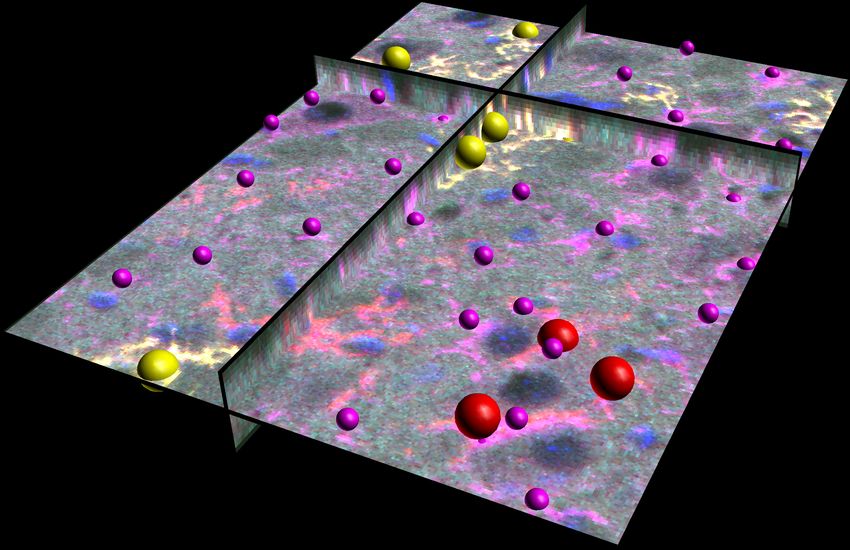
Author’s version of Falk et al. "U-Net – Deep Learning for Cell Counting, Detection, and
Morphometry". Nature Methods 16, 67–70 (2019), DOI:
http://dx.doi.org/10.1038/s41592-018-0261-2

The advancement of microscopy and sample preparation techniques leaves researchers with large
amounts of image data. The stacks of data promise additional insights, more precise analysis, and
more rigorous statistics, were there not the hurdles of quantification. Images must be converted
first into numbers before they are accessible for statistical analysis. Often this requires counting
thousands of cells with a certain marker or drawing the outlines of cells to quantify their shape
or the strength of a reporter. Such work is not much liked in the lab and, consequently, it is often
avoided. In neuroscientific studies applying optogenetic tools, for example, it is often requested
to quantify the number of opsin expressing neurons or the localization of newly developed opsins
within the cells. However, because of the effort, most studies are published without this information.
Is such quantification not a job that computers can do? Indeed it is. For decades, computer scientists
have developed specialized software that can lift the burden of quantification from researchers in
the life sciences. However, each lab produces different data and focuses on different aspects of the
data for their research question at hand. Thus, a new software must be built for each case. Deep
learning could change this situation. It learns the features relevant for the task from data rather than
being hard-coded. Therefore, software engineers need not set up a specialized software for a certain
quantification task. Instead, a generic software package can learn to adapt to the task autonomously
from appropriate data; data that researchers in the life sciences can provide by themselves.
Learning-based approaches caught the interest of the biomedical community already years ago.
Popular solutions like ilastik1a or the trainable WEKA segmentation toolkit2b allow training of seg-
mentation pipelines using generic hand-tailored image features. More recently, attention has shifted
towards deep learning which automatically extracts optimal features for the actual image analysis
task, lifting the need for feature design by experts in computer science3–5 . However, a wide-spread
use for quantification in the life sciences has been impaired by the lack of generic, easy-to-use soft-
ware packages. While the packages Aiviac and Cell Profiler6d already use deep learning models,
they do not allow training on new data. This restricts their application domain to a small range of
datasets. In the scope of image restauration, CSBDeep7 provides an ImgLib2e -based plugin with
models for specific imaging modalities and biological specimen. It allows to integrate externally
trained new restoration models. Another approach of bringing deep learning to the life sciences is
CDeep3M8 which ships a set of command line tools and tutorials for training and applying a resid-
ual inception network architecture for 3D image segmentation. They specifically address researchers
with occasional need for deep learning by providing a cloud-based setup that does not require a local
GPU.
The present work provides a generic deep-learning-based software package for cell detection and
cell segmentation. For our successful U-Net3 encoder-decoder network architecture, which has al-
ready achieved top ranks in biomedical data analysis benchmarks9 and which has been the basis of
many deep learning models in biomedical image analysis, we developed an interface that runs as
plugin in the popular ImageJ software10 (Supplementary note 1, Supplementary Software 1–4). In
contrast to all previous software packages of such kind, our U-Net can be trained and adapted to
new data and tasks by the users themselves using the familiar ImageJ interface (Fig. 1). This enables
application of U-Net to a wide range of tasks and makes it accessible for a wide set of researchers,
 a
   http://ilastik.org
 b
   https://imagej.net/Trainable_Weka_Segmentation
 c
   https://www.drvtechnologies.com/aivia6
 d
   http://cellprofiler.org/
 e
   https://imagej.net/ImgLib2

                                                   2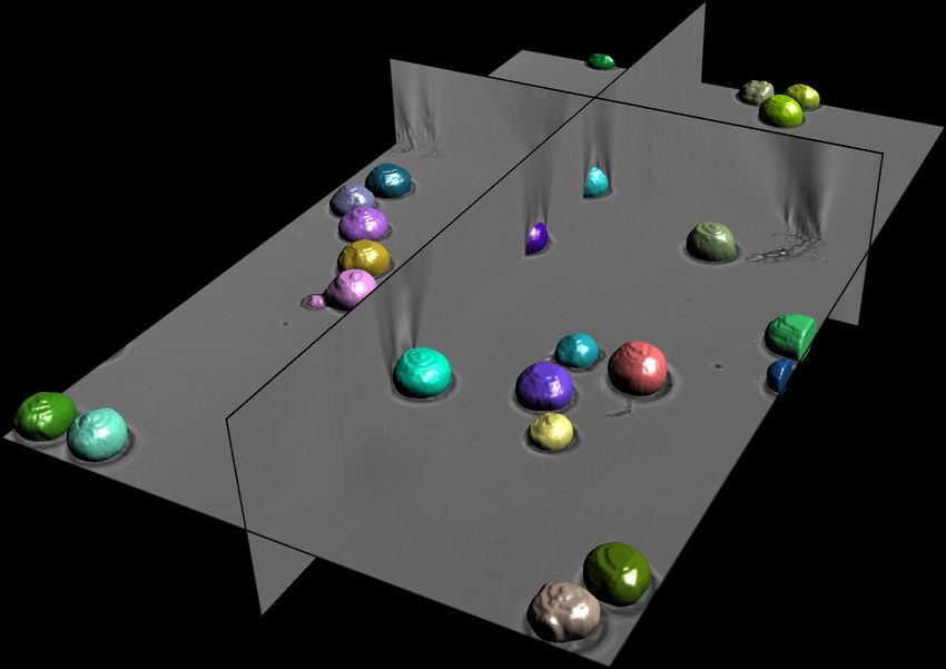
Author’s version of Falk et al. "U-Net – Deep Learning for Cell Counting, Detection, and
Morphometry". Nature Methods 16, 67–70 (2019), DOI:
http://dx.doi.org/10.1038/s41592-018-0261-2

who do not have experience with deep learning. For more experienced users the plugin offers an
interface to adapt aspects of the network architecture, and to train on data sets from completely
different domains. The software comes with a step-by-step protocol and tutorial that shows how to
annotate the data for adapting the network and that indicates typical pitfalls (Supplementary Note
2).
U-Net applies to general pixel classification tasks in flat images or volumetric image stacks with
one or multiple channels. Such tasks include detection and counting of cells, i.e., prediction of a
single reference point per cell, and segmentation, i.e., delineation of the outline of individual cells.
These tasks are a superset of the more wide-spread classification tasks, where the object of interest
is already localized and only its class label must be inferred. Although adaptation to the detection
and segmentation of arbitrary structures in biological tissue is possible given corresponding training
data, our experiments focused on cell images, where the flexibility of U-Net is shown on a wide
set of common quantification tasks, including detection in multi-channel fluorescence data of dense
tissue, and segmentation of cells recorded with different imaging modalities in 2D and 3D (Fig. 2
and Supplementary Note 3). In all shown cases, the U-Net would have saved the responsible sci-
entists much work. As cross-modality experiments show, the diversity in biological samples is too
large to ship a single software that can cover them all out-of-the-box (Supplementary note 3.2.2).
Thanks to the learning approach, U-Net’s applicability is extended from a set of special cases to
an unlimited number of experimental settings. The exceptionally precise segmentation results on
volumetric brightfield data, the annotation of which gets even human experts to their limits, is a par-
ticular strong demonstration of the capabilities of a deep-learning-based automated quantification
software (Fig. 2d and Supplementary Note 3.2.4).
Critics often stress the need for huge amounts of training data to train a deep network. In case of
U-Net, a base network trained on a diverse set of data and our special data augmentation strategy
allow adaptation to new tasks with only one or two annotated images (Online Methods). Only in
particularly hard cases, more than 10 training images are needed. Judgment whether a model is
adequately trained requires evaluation on a held-out validation set and successive addition of training
data until no significant improvement on the validation set can be observed (Supplementary Note
3.2.3). If computational resources allow, cross validation with randomly allocated train/test splits
avoids selection of a non-representative validation set at the expense of multiple trainings. The
manual effort that must be invested to adapt U-Net to a task at hand is typically much smaller than
what is needed for a minimal statistical analysis of the experimental data. In addition, U-Net offers
the possibility to run on much larger sample sizes without causing any additional effort. This makes
it particularly well-suited for automated large scale sample preparation and recording setups, which
are likely to become more and more common in the coming years.
U-Net was optimized for usability in the life sciences. The integration of the software in ImageJ
and a step-by-step tutorial make deep learning available to scientists without a computer science
background (Supplementary Videos 1–4). Importantly, the computational load is practicable for
common life science laboratory settings (Supplementary Note 1). Adaptation of the network to new
cell types or imaging modalities ranges from minutes to a few hours on a single computer with
a consumer GPU. If the dedicated compute hardware is not available in the lab, common cloud
services can be used.
Our experiments provide evidence that U-Net yields results comparable in quality to manual anno-
tation. One special feature of U-Net compared to other automatic annotation tools is the individual

                                                   3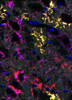
Author’s version of Falk et al. "U-Net – Deep Learning for Cell Counting, Detection, and
Morphometry". Nature Methods 16, 67–70 (2019), DOI:
http://dx.doi.org/10.1038/s41592-018-0261-2

Figure 1: Pipelines of the U-Net software. Left to right: input images and model → network train-
  ing/application on the local machine, a dedicated remote server or a cloud service → generated
  output. (a–c) Adaptation of the U-Net to newly annotated data using transfer learning; (a) Seg-
  mentation with regions of interest (ROI) annotations; (b) Segmentation with segmentation mask
  annotations. (c) Detection with multi-point annotations; (d–e) Application of the pre-trained or
  adapted U-Net to newly recorded data; (d) Segmentation; (e) Detection.

                                                4
Author’s version of Falk et al. "U-Net – Deep Learning for Cell Counting, Detection, and
Morphometry". Nature Methods 16, 67–70 (2019), DOI:
http://dx.doi.org/10.1038/s41592-018-0261-2
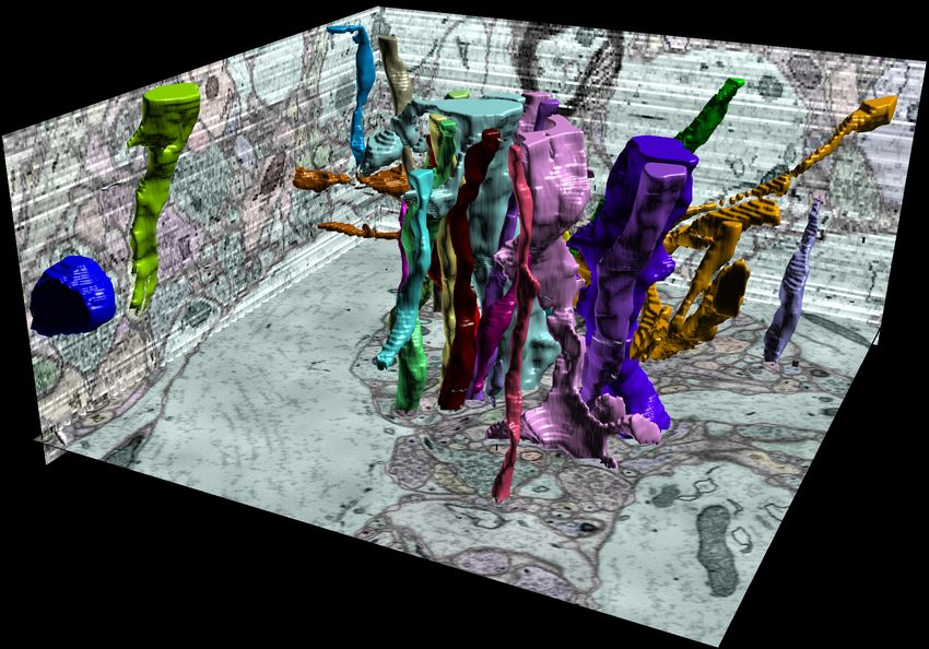
Figure 2: Example applications of the U-Net for 2D and 3D detection and segmentation. left: raw
data; right: U-Net output (with comparison to human annotation in the 2D cases). (a) Detection of
co-localization in two-channel epi-fluorescence images; (b) Detection of xFP-tagged microglial
cells in five-channel confocal image stacks. Magenta: all microglia; red, green, cyan: confetti
markers; blue: nucleus stain. (c) Cell segmentation in 2D images from fluorescence, DIC, phase
contrast and brightfield microscopy using one joint model. (d) Cell segmentation in 3D brightfield
image stacks. (e) Neurite segmentation in electron microscopy stacks.
5Author’s version of Falk et al. "U-Net – Deep Learning for Cell Counting, Detection, and
Morphometry". Nature Methods 16, 67–70 (2019), DOI:
http://dx.doi.org/10.1038/s41592-018-0261-2
influence of the annotator. This is advantageous as typically researchers develop individual proto-
cols in which multiple parameters are taken into account without being explicitly mentioned. Due
to the complexity of these labeling rules they cannot be reproduced by common automatic labeling
tools. This advantage can also be turned into a disadvantage: U-Net learns from the provided exam-
ples. If these examples are not representative for the actual task or if the manual annotation in these
examples is of low quality and inconsistent, U-Net will either fail to train or will reproduce incon-
sistent annotations on new data. This could also serve as a quality check of the manual annotations.
Together, U-Net cannot correct for low-quality human annotations but is a tool to apply individual
labeling rules to large data sets and thereby can save manual annotation effort in a vast variety of
quantification tasks.
1 Acknowledgements
This work was supported by the German Federal Ministry for Education and Research (BMBF)
through the MICROSYSTEMS project (0316185B): TF, AD; and the Bernstein Award 2012 (01GQ2301):
ID; by the Federal Minstry for Economic Affairs and Energy (ZF4184101CR5): AB; by the Deutsche
Forschungsgemeinschaft (DFG) through the collaborative research center KIDGEM (SFB 1140):
DM, ÖC, TF, OR; the clusters of excellence BIOSS (EXC 294): TF, DM, RB, AA, YM, DS, TLT,
MP, KP, MS, TB, OR; and BrainLinks-Brain-Tools (EXC 1086): ZJ, KS, ID, TB; as well as grants
DI 1908/3-1: JD; DI 1908/6-1: ZJ, KS; and DI 1908/7-1: ID; by the Swiss National Science Foun-
dation (SNF Grant 173880): AA; by the ERC Starting Grant OptoMotorPath (338041): ID; and by
the FENS-Kavli Network of Excellence (FKNE): ID. We thank F. Prósper, E. Bártová, V. Ulman,
D. Svoboda, G. van Cappellen, S. Kumar, T. Becker and the Mitocheck consortium for providing a
rich diversity of datasets through the ISBI segmentation challenge. We thank P. Fischer for manual
image annotations. We thank S. Wrobel for tobacco microspore preparation.
2 Author Contributions
TF, DM, RB, YM, ÖC, TB and OR selected and designed the computational experiments.
TF, RB, DM, YM, AB and ÖC performed the experiments, RB, DM, YM, AB (2D) and TF, ÖC
(3D).
R.B., Ö.C., A.A., T.F. and O.R. implemented the U-Net extensions into caffe.
T.F. designed and implemented the Fiji plugin.
D.S. and M.S. selected, prepared and recorded the Keratinocyte dataset PC3-HKPV.
T.F. and O.R. prepared the airborne pollen dataset BF1-POL.
A.D., S.W., O.T., C.D.B. and K.P. selected, prepared and recorded the protoplast and microspore
datasets BF2-PPL and BF3-MiSp.
T.L.T. and M.P. prepared, recorded and annotated the data for the microglial proliferation experi-
ment.
J.D. and Z.J. selected, prepared, and recorded the optogenetic data set.
I.D., J.D., and Z.J. manually annotated the optogenetic data set.
I.D., T.F., D.M., R.B., Ö.C., T.B. and O.R. wrote the manuscript.
6Author’s version of Falk et al. "U-Net – Deep Learning for Cell Counting, Detection, and
Morphometry". Nature Methods 16, 67–70 (2019), DOI:
http://dx.doi.org/10.1038/s41592-018-0261-2
3 Competing financial interests
We declare no competing financial interests.
4 Ethics compliance statement
We declare that we complied with all relevant ethical regulations.
References
1. Sommer, C., Straehle, C., Koethe, U. & Hamprecht, F. A. Ilastik: Interactive learning and
segmentation toolkit in Biomedical Imaging: From Nano to Macro, 2011 IEEE International
Symposium on Biomedical Imaging (2011), 230–233.
2. Arganda-Carreras, I. et al. Trainable Weka Segmentation: a machine learning tool for mi-
croscopy pixel classification. Bioinformatics 33, 2424–2426 (2017).
3. Ronneberger, O., Fischer, P. & Brox, T. U-Net: Convolutional Networks for Biomedical Image
Segmentation in Medical Image Computing and Computer-Assisted Intervention (MICCAI)
9351 (2015), 234–241.
4. Rusk, N. Deep learning. Nature Methods 13, 35–35 (2016).
5. Webb, S. Deep Learning For Biology. Nature 554, 555–557 (2018).
6. Sadanandan, S. K., Ranefall, P., Le Guyader, S. & Carolina, W. Automated Training of Deep
Convolutional Neural Networks for Cell Segmentation. Scientific Reports 7, 7860 (2017).
7. Weigert, M. et al. Content-Aware Image Restoration: Pushing the Limits of Fluorescence Mi-
croscopy tech. rep. (Center for Systems Biology Dresden (CSBD), Dresden, Germany, 2017).
8. Haberl, M. G. et al. CDeep3 – Plug-and-Play cloud-based deep learning for image segmenta-
tion. Nature Methods 15, 677–680 (2018).
9. Ulman, V. et al. An objective comparison of cell-tracking algorithms. Nature Methods 14,
1141–1152 (2017).
10. Schneider, C. A., Rasband, W. S. & Eliceiri, K. W. NIH Image to ImageJ: 25 years of image
analysis. Nature Methods 9, 671–675 (2012).
11. Çiçek, Ö., Abdulkadir, A., Lienkamp, S. S., Brox, T. & Ronneberger, O. 3D U-Net: Learn-
ing dense volumetric segmentation from sparse annotation in Medical Image Computing and
Computer-Assisted Intervention (MICCAI) 9901 (2016), 424–432.
12. He, K., Zhang, X., Ren, S. & Sun, J. Delving Deep into Rectifiers: Surpassing Human-Level
Performance on ImageNet Classification. CoRR abs/1502.01852 (2015).
13. Everingham, M., Van Gool, L., Williams, C. K. I., Winn, J. & Zisserman, A. The Pascal Vi-
sual Object Classes (VOC) Challenge. International Journal of Computer Vision 88, 303–338
(2010).
14. Maška, M. et al. A benchmark for comparison of cell tracking algorithms. Bioinformatics 30,
1609–1617 (2014).
7Author’s version of Falk et al. "U-Net – Deep Learning for Cell Counting, Detection, and
Morphometry". Nature Methods 16, 67–70 (2019), DOI:
http://dx.doi.org/10.1038/s41592-018-0261-2
C 64 64
192 128 128 K
Output segmentation map
Input image tile
(C channels)
(K classes)
3602
3582
3562
3562
5402
5382
5362
128 128
er
256 128
En
cod
cod
De
er
1842
1822
1802
2682
2662
2642
256 256 512 256
convolution 3x3, ReLU
962
942
922
1322
1302
1282
512 512 1024 512 max pooling 2x2 (stride 2)
up-convolution 2x2 (stride 2)
642
622
602
522
502
482
1024 convolution 1x1
copy & crop
302
282
262
Figure 3: The U-Net architecture at the example of the 2D cell segmentation network. An image tile
with C channels is input to the network on the left (blue box). The K-class soft-max segmentation
is output on the right (yellow box). Blocks show the computed feature hierarchy. Numbers atop
each network block: number of feature channels; numbers left to each block: spatial feature map
shape in pixels. Yellow arrows: Data flow.
Online Methods
M1 Network architecture
The U-Net is an encoder-decoder-style neural network solving semantic segmentation tasks end-
to-end (Fig. 3). Its 26 hidden layers can be logically grouped in two parts: An encoder that takes
an image tile as input and successively computes feature maps at multiple scales and abstraction
levels yielding a multi-level, multi-resolution feature representation; a decoder that takes the feature
representation and classifies all pixels/voxels at original image resolution in parallel. Layers in the
decoder gradually synthesize the segmentation starting at low-resolution feature maps (describing
large scale structures) up to full-resolution feature maps (describing fine scale structures).
The encoder is a typical convolutional neural network. It consists of the repeated application of two
convolutions (without padding), each followed by a leaky rectified linear unit (ReLU) with leakage
factor 0.1 and a max-pooling operation with stride two halving the resolution of the resulting feature
map. Convolutions directly following down-sampling steps double the number of feature channels.
The decoder consists of repeated application of an up-convolution (an up-convolution is equivalent
to a bed-of-nails up-sampling by a factor of two followed by a convolution with edge length two)
that halves the number of feature channels, then concatenation with the cropped encoder feature
map at corresponding resolution and two convolutions each followed by leaky ReLUs with leakage
factor 0.1.
At the final layer a 1×1 convolution is used to map feature vectors to the desired number of classes
8Author’s version of Falk et al. "U-Net – Deep Learning for Cell Counting, Detection, and
Morphometry". Nature Methods 16, 67–70 (2019), DOI:
http://dx.doi.org/10.1038/s41592-018-0261-2
K.
For training, the final K-class scores are transformed to pseudo-probabilities with soft-max before
they are compared to the ground truth annotations in one-hot encoding using cross entropy.
If not explicitly mentioned, operations are isotropic and convolutions use a kernel edge length of
three pixels. We only use the valid part of each convolution, i.e. the segmentation map only contains
the pixels, for which the full context is available in the input image tile.
This fully convolutional network architecture allows to freely choose the input tile shape with the
restriction that edge lengths of feature maps prior to max pooling operations must be even. This
implies the possibility to process arbitrarily large images using an overlap-tile strategy where the
stride is given by the output tile shape. To predict pixels in the border region of an image, missing
context is extrapolated by mirroring the input image.
The ImageJ plugin presents only valid tile shapes to the user. For 2D networks the user can also let
the plugin automatically choose an optimal tiling based on the available GPU memory. For this the
amount of memory used by the given architecture for different tile sizes must be measured on the
client PC beforehand and corresponding information stored to the model definition file using the
provided MATLAB script caffe-unet/matlab/unet/measureGPUMem.m.
M1.1 3D U-Net
The 3D U-Net architecture for volumetric inputs is only a slight modification of its 2D counterpart.
First, input tiles have a shape of 236×236×100 voxels (vx). Secondly, due to memory limitations,
we half the number of output features of each convolution layer except for the last up-convolution
step that only produces 32 channels. Thirdly, to deal with anisotropic image voxel sizes, convolu-
tions and pooling at the finest resolution levels are 2D until voxel extents are roughly isotropic. At
all remaining resolution levels operations are applied along all three dimensions.
M2 Weighted soft-max cross-entropy loss
We use pixel-weighted soft-max cross-entropy loss to allow to change the influence of imbalanced
classes in semantic segmentation. The loss is computed as
X eŷy(x) (x)
l (I) := − w (x) log PC
ŷc (x)
x∈Ω c=0 e
where x is a pixel in image domain Ω, ŷc : Ω → R is the predicted score for class c ∈ {0, . . . , C},
C is the number of classes, y : Ω → {0, . . . , C} is the true class label. With this, ŷy(x) (x) is the
predicted score for the ground truth class at position x. As defined above, w : Ω → R≥0 is the
pixel-wise loss weight.
We employ loss weighting to optimize class-balancing and handle regions without annotations (in
the following termed "ignored regions") using weight map wbal . We additionally enforce instance
separation using weight wsep as described in the following sections. The final loss weights are then
given by
9Author’s version of Falk et al. "U-Net – Deep Learning for Cell Counting, Detection, and
Morphometry". Nature Methods 16, 67–70 (2019), DOI:
http://dx.doi.org/10.1038/s41592-018-0261-2
0
w (x) := wbal + λwsep
where λ ∈ R≥0 controls the importance of instance separation.
M2.1 Class balancing and regions with unknown ground truth
In our images most pixels belong to the background class, and in many cases this class is homoge-
neous and easy to learn. Therefore, we reduce the weight of background pixels by factor vbal ∈ [0, 1]
compared to foreground pixels resulting in the class balancing weight function
1
y (x) > 0
wbal (x) := vbal y (x) = 0
0 y (x) unknown (i.e. ignored regions).
We observed slightly better segmentation results when replacing the step-shaped cutoff at the edges
of foreground objects by a smoothly decreasing Gaussian function for the weighted loss computa-
tion, therefore we define
1 y (x) > 0
d2 (x)
0
wbal (x) := vbal + (1 − vbal ) · exp − 2σ1 2 y (x) = 0
bal
0 y (x) unknown (i.e. ignored)
where d1 (x) is the distance to the closest foreground object and σbal is the standard deviation of the
Gaussian.
For the detection tasks we added rings/spherical shells of ignored regions with outer radius rign
around annotated locations to both wbal and wbal 0 . These regions help to stabilize the detection
process in case of inaccurate annotations, but are not essential to the approach.
M2.2 Instance segmentation
Semantic segmentation classifies pixels/voxels of an image. Therefore, touching objects of the same
class will end up in one joint segment. Most often we want to measure properties of individual object
instances (e.g. cells). Therefore we must turn the pure semantic segmentation into an instance-aware
semantic segmentation. For this we insert an artificial one pixel wide background ridge between
touching instances in the ground truth segmentation mask (Fig. 4a).
To force the network to learn these ridges we increase their weight in the loss computation such that
the thinnest ridges get the highest weights. We approximate the ridge width at each pixel by the sum
of the distance d1 to its nearest instance and the distance d2 to its second-nearest instance. From this
we compute the weight map as
!
(d1 (x) + d2 (x))2
wsep (x) := exp − 2
,
2σsep
which decreases following a Gaussian curve with standard deviation σsep (Fig. 4b).
10Author’s version of Falk et al. "U-Net – Deep Learning for Cell Counting, Detection, and
Morphometry". Nature Methods 16, 67–70 (2019), DOI:
http://dx.doi.org/10.1038/s41592-018-0261-2
a b
40
30
20
10
Figure 4: Separation of touching cells using pixel-wise loss weights. (a) Generated segmentation
mask with one pixel wide background ridge between touching cells (white: foreground, black:
background) (b) Map showing pixel-wise loss weights to enforce the network to separate touching
cells.
a b c
75
100µm 225
375
525
75 225 375 525
Figure 5: Training data augmentation by random smooth elastic deformation. (a) Upper left: Raw
image; Upper right: Labels; Lower Left: Loss Weights; Lower Right: 20µm grid (for illustration
purpose only) (b) Deformation field (black arrows) generated using bicubic interpolation from
a coarse grid of displacement vectors (blue arrows; magnification: 5×). Vector components are
drawn from a Gaussian distribution (σ = 10px). (c) Back-warp transformed images of (a) using
the deformation field.
M3 Tile sampling and augmentation
Data augmentation is essential to teach the expected appearance variation to the neural network
with only few annotated images. To become robust to translations and to focus on relevant regions
in the images, we first randomly draw spatial locations of image tiles that are presented to the
network from a user-defined probability density function (pdf). For all our experiments we used the
normalized weight map wbal for sampling the spatial location, i.e. foreground objects are presented
to the network ten times more often (according to our selection of vbal = 0.1) than background
regions and tiles centered around an ignore region are never selected during training. Then, we draw
a random rotation angle (around the optical axis in 3D) from a uniform distribution in a user-defined
range. Finally, we generate a smooth deformation field by placing random displacement vectors with
11Author’s version of Falk et al. "U-Net – Deep Learning for Cell Counting, Detection, and
Morphometry". Nature Methods 16, 67–70 (2019), DOI:
http://dx.doi.org/10.1038/s41592-018-0261-2
user-defined standard deviation of the magnitude for each component on a very coarse grid. These
displacement vectors are used to generate a dense full-resolution deformation field using bicubic
interpolation (Fig. 5). Rigid transformations and elastic deformations are concatenated to look-up
intensities in the original image during tile generation.
We additionally apply a smooth strictly increasing intensity transformation to become robust to
brightness and contrast changes. The intensity mapping curve is generated from a user-defined num-
ber of equidistant control points in the normalized [0, 1] source intensity range. Target intensities at
the control points are drawn from uniform distributions with user defined ranges. The sampling pro-
cess enforces intensities at subsequent control points to increase and spline interpolation between
the control points ensures smoothness.
All data augmentation is applied on-the-fly to input image, labels and weight maps during network
training11 .
M4 Training
All networks were trained on an nVidia TITAN X with 12GB GDDR5 RAM using cuda 8 and
cuDNN 6 with caffe after applying our proposed extensions. Thep initial network parameters are
drawn from a Gaussian distribution with standard deviation σ = 2/nin , where nin is the number
of inputs of one neuron of the respective layer12 .
For all experiments, raw image intensities per channel were normalized to the [0, 1] range before
training using
I − min {I}
Iˆ :=
max {I} − min {I}
where I is the raw and Iˆ the normalized intensity.
M5 Transfer learning
Adaptation of a pre-trained U-Net to a new dataset using annotated data is called transfer learning
or finetuning. Transfer learning leverages the knowledge about the different cell datasets already
learned by the U-Net and usually requires considerably less annotated data and training iterations
compared to training from scratch.
Transfer to a new dataset is based on the same training protocol as described above. All the user
must provide are raw images and corresponding annotations as ImageJ ROIs or pixel masks (De-
tection: One Multi-point ROI per class and image; Segmentation: One regional ROI per object or
pixel masks) (Supplementary Section B). The plugin performs image re-scaling, pixel weight w(x)
generation, and parametrization of the caffe training software.
12Author’s version of Falk et al. "U-Net – Deep Learning for Cell Counting, Detection, and
Morphometry". Nature Methods 16, 67–70 (2019), DOI:
http://dx.doi.org/10.1038/s41592-018-0261-2
M6 Evaluation Metrics
M6.1 Object Intersection over Union
The intersection over union (IoU) measures how well a predicted segmentation matches the corre-
sponding ground truth annotation by dividing the intersection of two segments by their union. Let
S := {s1 , . . . , sN } be a set of N pixels. Let G ⊂ S be the set of pixels belonging to a ground truth
segment and P ⊂ S be the set of pixels belonging to the corresponding predicted segment. The IoU
is defined as
|G ∩ P|
MIoU (G, P) = .
|G ∪ P|
IoU is a widely used measure, e.g. in the Pascal VOC challenge13 or the ISBI cell tracking chal-
lenge14 . MIoU ∈ [0, 1] with 0 meaning no overlap at all and 1 meaning a perfect match. In our
experiments, a value of ∼ .7 indicates a good segmentation result, and a value of ∼ .9 is close to
human annotation accuracy.
We first determine the predicted objects by performing a connected component labelling with 8-
neighborhood on the binary output of the U-Net. This yields candidate segments Si . Then we
compute the IoU for every pair of output and ground truth segments Gj : MIoU (Si , Gj ) and ap-
ply the Hungarian algorithm on MIoU to obtain 1:1 correspondences maximizing the average IoU.
Unmatched segments or matches with zero IoU are considered false positives and false negatives,
respectively. The average IoU is computed based on the ground truth annotations, i.e. false negatives
contribute to the average IoU with a value of 0. False positives, however, are not considered in the
average IoU.
In the supplementary material we provide a detailed analysis of false positive segmentations pro-
duced by the U-Net.
M6.2 F-measure
We measure the quality of a detector using the balanced F1 score (denoted as F-measure) which is
the harmonic mean of precision and recall. Let G be the set of true object locations and P be the set
of predicted object locations. Then precision and recall are defined as
|G ∩ P | |G ∩ P |
Precision := and Recall := .
|P | |G|
The F-measure is then given by
Precision · Recall
F1 = 2 · .
Precision + Recall
Pixel-accurate object localization is almost impossible to reach, therefore, we introduce a tolerance
dmatch for matching detections and annotations. To get one-to-one correspondences, we first com-
pute the pairwise distances of ground truth positions to detections. Predictions with distance greater
13Author’s version of Falk et al. "U-Net – Deep Learning for Cell Counting, Detection, and
Morphometry". Nature Methods 16, 67–70 (2019), DOI:
http://dx.doi.org/10.1038/s41592-018-0261-2
than dmatch to any ground truth position can be directly classified as false positive. Similarly ground
truth positions without detections in the dmatch range are classified as false negatives. We apply
the Hungarian algorithm to the remaining points to obtain an assignment of predictions to ground
truth positions minimizing the total sum of distances of matched positions. Correspondences with
distance greater than dmatch and unmatched positions in either ground truth or prediction are treated
as false negative/false positive detections as before.
M7 Code availability
We provide pre-built binary versions of the U-Net caffe extensions for Ubuntu Linux 16.04 at
https://lmb.informatik.uni-freiburg.de/resources/opensource/unet/. We
additionally provide our changes to the source code of the publicly available caffe deep learning
frameworkf as patch file with detailed instructions on how to apply the patch and build our caffe
variant from source in the supplementary material.
Binary installation only requires to unpack the archive and install required third-party libraries which
can be done within few minutes on an Ubuntu 16.04 machine depending on your internet connection
for fetching the packages.
Building from scratch requires to install the dependent development libraries and checkout the given
tagged version of the BVLC caffe master branch and apply the patch. With "normal" internet connec-
tion, package installation is a matter of few minutes. Cloning the BVLC master repository requires
less than a minute, applying the patch imposes no measurable overhead. Configuring and building
the package requires approximately ten to fifteen minutes.
The U-Net segmentation plugin for Fiji/ImageJ is available at http://sites.imagej.net/
Falk/plugins/ or through the ImageJ updater within Fiji. Source code is included in the plugin
jar File Unet_Segmentation.jar. Installation using the Fiji updater requires only a few seconds.
The trained caffe-models for the 2d- and 3d-U-Net are available at https://lmb.informatik.
uni-freiburg.de/resources/opensource/unet/.
M8 Data availability
The datasets F1-MSC, F2-GOWT1, F3-SIM, F4-HeLa, DIC1-HeLa, PC1-U373, and PC2-PSC are
from the ISBI Cell Tracking Challenge 201514 . Information on how to obtain the data can be found
at http://celltrackingchallenge.net/datasets.html and currently requires free-
of-charge registration for the challenge.
The datasets PC3-HKPV, BF1-POL, BF2-PPL, and BF3-MiSp are custom and are available from
the corresponding author upon reasonable request.
Datasets for the detection experiments partially contain unpublished sample preparation protocols,
and are currently not freely available. Upon protocol publication datasets will be made available on
request-basis.
f
https://github.com/BVLC/caffe
14You can also read