Motion Estimation and Segmentation of Natural Phenomena - BMVC 2018
←
→
Page content transcription
If your browser does not render page correctly, please read the page content below
CHEN, LI, HALL: MOTION ESTIMATION AND SEGMENTATION OF NATURAL PHENOMENA 1

Motion Estimation and Segmentation
of Natural Phenomena
Da Chen                                                        Department of Computer Science
da.chen@bath.edu                                               University of Bath
                                                               Bath, UK
Wenbin Li                                                      Imperial College London
wenbin.li@imperial.ac.uk                                       London, UK
Peter Hall                                                     CAMERA
P.M.Hall@bath.ac.uk                                            University of Bath
                                                               Bath, UK

                                                        Abstract

            Dense motion estimation for dynamic natural phenomena (water, smoke, fire, etc.) is a
        significant open problem. Current approaches tend to be either general, giving poor results, or
        specialise in one phenomenon and fail to generalise. Segmentation of phenomena is also an open
        problem. This paper describes an approach to estimate dense motion for dynamic phenomena
        that is simple, general, and which yields state of the art results. We use our dense motion field
        to segment phenomena to above state of the art levels. We demonstrate our contributions using
        lab-based video, video from a public dataset, and from the internet.

1 Introduction
Accurate, dense motion estimation is a long-standing problem in Computer Vision. Several decades
of research have produced impressive results. Motion estimation over a wide variety of different
types of object is now possible: rigid bodies, articulated bodies, soft bodies. Yet a simple but general
motion estimator for natural phenomena (smoke, fire, etc) currently remains unavailable. Similar
remarks apply to segmentation where many problem have been solved but the segmentation of natural
phenomena remains difficult.
    Simple but general solutions to these problems would benefit many diverse application areas. For
example Computer Graphics has applications in both post-production [16, 18, 26] and model acqui-
sition [22]. In atmospheric research, there are applications for storm identification and forecast [21],
forecast and tracking the evolution of convective systems [37] and rain cloud tracking [5]. Our motiva-
tion derives from model acqusition and editing in the creative sector. Our approach using “skeletons”
included a desire to provide entities to support editing, but a discussion of editing would take us well
beyond the focus of this paper: the computer vision problems of flow estimation and segmentation.
    This contributions of this paper are as follows. First to describe a simple method using “skeletons”
for sparse flow estimation with an upgrade to dense flow estimation, and in particular to show that
it generalises to several phenomena. Skeletons are sparse topographical maps over the phenomena.
Empirical testing using laboratory based data, a public dataset for natural phenomena, and video from
the internet “in the wild") show our method significantly improve state-of-the-art accuracy above a rep-
resentative range of both well established and current methods. Second, we show how to use our dense
flow solution, including skeletons, to segment natural phenomena, exceeding state-of-the-art solutions.

 c 2018. The copyright of this document resides with its authors.
It may be distributed unchanged freely in print or electronic forms.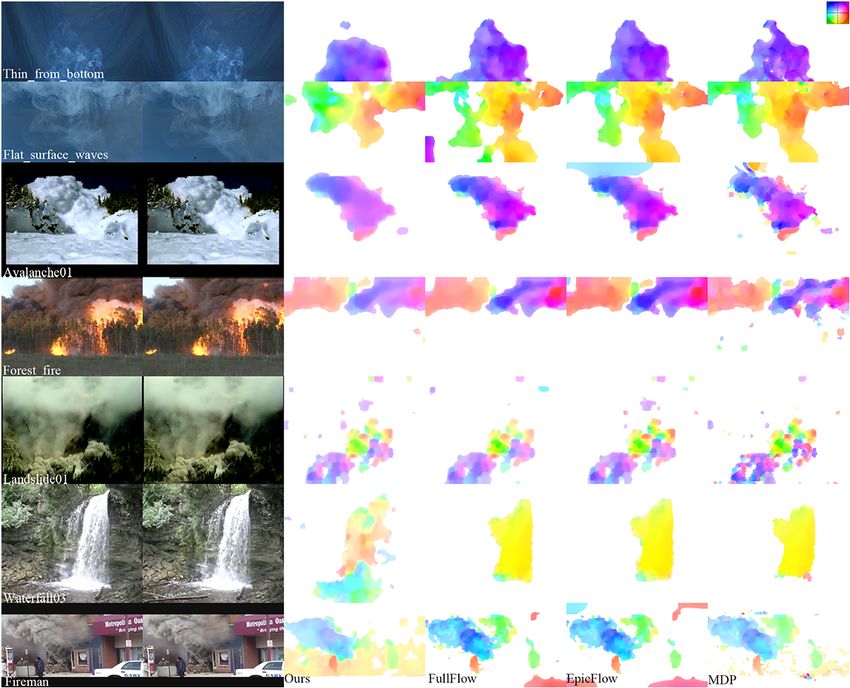
2 CHEN, LI, HALL: MOTION ESTIMATION AND SEGMENTATION OF NATURAL PHENOMENA

2 Related Work
Optical flow [19] describes dense motion. Significant effort has been expended on real-world chal-
lenges e.g. large pixel displacement [7], non-rigid deformation [15] and rapid optimization [9, 14, 29],
etc.
    Most optical flow estimation approaches are based on a variational model which combines a data
term with a regularising term. The former encodes a brightness constancy assumption while the
latter constraints how the motion field can vary over space. Fluid motion is non-rigid and violates
the brightness constancy assumption; but careful choice of the regularising term boosts performance.
Example appraaches include Auroux et al. [3] who utilise a group-wise appearance prior to regularize
the flow; also Corpetti et al. [11] who impose divergence and curl smoothness to constraint fluid
motion. Stronger physical models appeal to the Navier-Stokes (NS) equations to design a regulariser.
Doshi et al. [13] replace the normal smoothness term with Navier-Stokes (NS) equation, which
preserves general motion behaviour but often over-smooths details. To further smooth the motion,
Anumolu et al. [2] propose vorticity confinement which blurs the internal boundaries. Li et al.. [23]
claim that NS equations can be applied together with 3D flow prediction in order to improve precision.
    Others have used physical properties more directly. Sakaino [30] generates the properties of
wave using sinusoidal functions to achieve dense fluid motion. Refractive properties are used in
[20, 42]. These approaches give high performance in the laboratory environments but lead to errors
on real-world cases.
    Recent work has proven the importance of high-quality sparse flow estimations to initiate upgrades
to dense flow. Revaud et al. [29] propose a novel sparse to dense interpolation to post-process the
matching result of DeepMatch [39] and use it as an initial input for standard optical flow energy
minimization process. Chen et al. [9] further improve the sparse match result and got state-of-the-art
result using the same framework as EpicFlow [29]. Such work is of relevance here because we too
begin with a sparse estimate, which is then upgraded to a dense estimate.
    Segmentation of natural phenomena is difficult because they are diffuse, translucent, often have ill
defined borders, and usually form part of a complex scene. There are some works in the literature on
the subject. Xu et al. [40], and later, Ochs et al. [24] use multiple frames. Papazoglou and Ferrari [27]
use optical flow to track superpixels over time to establish temporal coherence and further achieve
the fast foreground segmentation. Teney et al. [34, 35] propose custom spatio-temporal filters, over
a time window of about 7 or 8 frames, to separate spatial and temporal patterns – a learnable metric
improves their segmentation on highly dynamic objects. Most recently, Cheng et al. [10] integrate
segmentation and motion estimation by proposing an end-to-end trainable network; they provide
good results in both segmentation and motion estimation. Due to the lack of ground-truth data, we
cannot train this network on natural phenomena sequences, hence during experiments we applied
the model provided by the authors to obtain test results.
    Our flow estimator differs from all of the above. Its aims to be less specific than approaches
premised on fluids, so we cannot appeal to Navier-Stokes or similar physical equations. As explained
next, we use a two-stage approach, the first of which completely abandons the brightness constacy
assumption to produce a sparse but global flow. This global flow then provides a starting point for
a dense estimation that does use brightness constancy. Our algorithm for segmentation is also unique:
it re-purposes the “skeletons” from the flow estimate, and requires only a pair of frames to exceed
state of the art results.
3 Flow Estimation
As observed in Section 2, current motion estimation methods for natural phenomena either make weak
but (in this case) invalid assumptions such as brightness constancy, or else make strong assumptions
regarding the behaviour of fluids. We adopt neither of these to estimate a global flow. Instead, our
method assumes that the global shape of the phenomena under observation changes little between
frames. Specifically, we assume topographical maps, here called skeletons, in adjacent frames are
CHEN, LI, HALL: MOTION ESTIMATION AND SEGMENTATION OF NATURAL PHENOMENA 3
=16 =4 =1 1
Input 0
Skeleton
=8 =2 =0.5
Figure 1: Given an input frame, a weighted skeleton is aggregated from binary skeletons generated
different filtering scales. Although we use the as example to explain skeleton generation, the same
applies to other natural phenomena.
similar. Our skeletons are maps of local intensity maxima, because this typically corresponds the
the densest region of smoke / steam / fire etc. These skeletons do not change much between frames
even if brightness changes it is likley to remain locally maximaly, and being sparse makes skeletons
easy to use to construct a sparse flow.
Our approach has three main steps: (1) construct a skeleton for each of two frames; (2) estimate a
sparse flow; (3) upgrade sparse flow to dense flow (at which point we do allow brightness constancy
to influence the solution). For segmentation, we segment with the aid of the skeleton. As results
show, we obtain excellent results over a range of phenomena and videos from different sources.
3.1 Skeleton Construction
Constructing a skeleton is straightforward. Given a gray scale image, we blur it with a Gaussian
kernel of scale σ, to obtain f (.). Next, we mark local horizontal maxima. There is horizontal maxima
at pixel (x,y) if f (x−1,y) ≤ f (x,y) ≥ f (x+1,y). Similarly, mark local vertical maxima over pixel
columns. Finally, we combine these maps of maxima to make a binary skeleton by combining them
with an ‘or’ operator. We construct a weighted multi-scale skeleton by the aggregation of binary
skeletons at different scales:
1 N
h(x)= ∑ h j (x), (1)
N j=1
with h j being a binary skeleton image under blurring kernel σ j , and x is a point in the image. The
result of this is a multi-scale skeleton that tends to emphasise stable structures within the phenomenon:
higher values of the mutli-scale skeleton indicate locations that are more stable over scale. Figure 1
illustrates the skeleton building process.
3.2 Sparse Flow Estimation
We begin flow estimation by assuming R that the motion of observed phenomena is subject to a very
general transfer of mass ρt+dt (y)= x∈ℜ3 φ(y,x)ρt (x)dx in which ρ(.) is local density, ρt (x)dx is
local mass, and φ is a mass transfer function that includes systematic motion, diffusion, etc. This
is at best very hard to solve. Instead, we further assume points x and y lie in the plane ℜ2, that local
density is proportional to observed pixel brightness, and we consider only points on one multi-scale
skeleton. Specifically, we estimate the expected location of each point x on a topographic skeleton
S1 ⊂ℜ2 when attracted by all points y on a topographic skeleton S2 ⊂ℜ2:
E[y|x]= ∑ yp(y|x). (2)
y∈S2
The expected point E[y|x] is not constrained to lie on skeleton S2, but it is global in the sense that
it takes all S2 points into account. It does not rely on brightness, nor does it require any optimisation,
so is very fast to compute.
The definition of p(y|x) is important. It is defined using spatial distance and intensity of the
skeletal pixels, similar to a bilateral filter [36]
p(y|x)∝N (x|y,Cy)N (h(x)|h(y),σv). (3)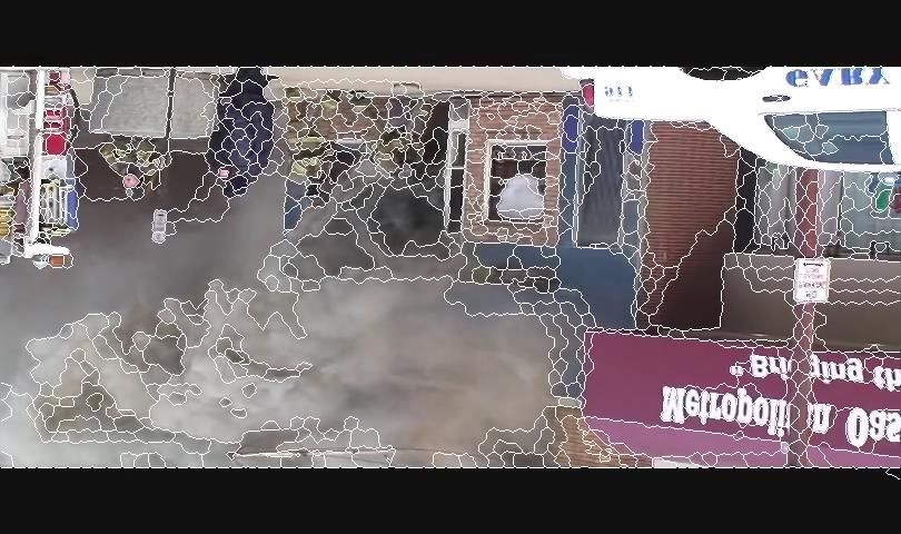
4 CHEN, LI, HALL: MOTION ESTIMATION AND SEGMENTATION OF NATURAL PHENOMENA

in which h(.) is the value at a point in a multi-valued skeletal image (Eqn. 1). The term using them
encourages a match between skeletal parts of about equal stability; the variance σv matters little;
we set σv = 1. The spatial part of the attraction depends on a covariance C. For this we use a
non-isotropic Gaussian that is aligned so that its longest principle axis is normal to the skeleton S2
at y. The covariance matrix Cy =ULU T is specified by:
                                        U = [n̂, t̂],                                                (4)
                                         L = σdiag([s, 1]).                                          (5)
The value of σ determines the effective range of the attraction, we set σ = 1, but a wide range of
values suffice. The scale s determines the weight of the axis normal to the skeleton relative to the
tangential axis. An isotropic Gaussian tends to attract points more strongly to the centre of skeletal
lines, a tendency we wish to avoid. Therefore, we adopt an elliptical covariance with long-axis normal
to the local skeleton mitigates against a build-up of probability density towards the centre of skeletal
lines. A wide range of s value works well, in our experiments we set s=10.
3.2.1 Improving the sparse estimate
We improve on the sparse estimate by also considering the ‘backward’ process (similar to [25]).
That is, we also consider E[x|y]. In particular, we assume that the underlying physics governing
the phenomenon are symmetric in time. Therefore, we estimate both sparse motion both forward
and backward in time, and maintain only consistent results. In a little more detail, we consider sets
with ‘forward elements’ (x ∈ S1,E[y|x]) and ‘backward elements’ (x0 ∈ S2,E[y0|x0]). To check the
consistency, we use
                                               2                    2
                            x−E[y0|x0] + E[y|x]−x0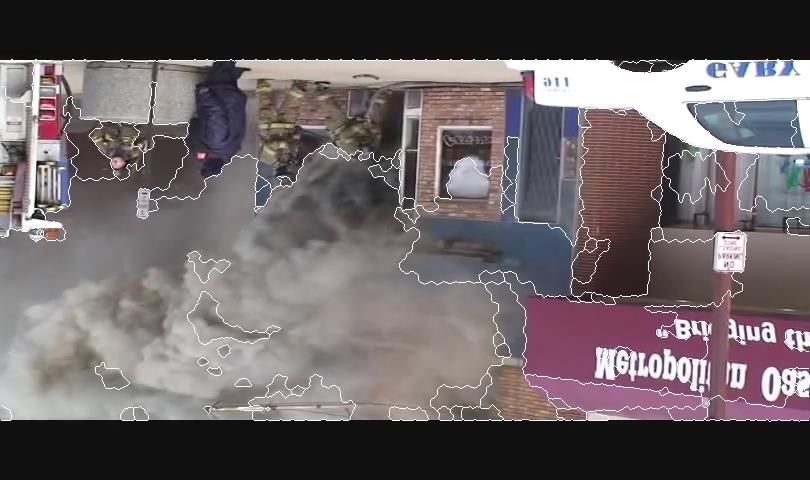
CHEN, LI, HALL: MOTION ESTIMATION AND SEGMENTATION OF NATURAL PHENOMENA 5

      Original Frame     SuperPixel (SP)   SP on L*A*B Color   SP Merged on Motion Final Segmentations

Figure 2: Steps in frame segmentation, each step uses agglomerative clustering to merge super-pixels
into image segments; colour, motion and skeletal density are used respectively.

 where f∗ denotes the input images and v represents the smoothed flow field in between; ∇ =
(∂xx ,∂yy)T is a spatial gradient and φ(s)=ε 2log(1+s2/ε 2) with ε =2 penalizes the flow gradient
norm. The energy function was defined as a combination of a data term (brightness constancy and
gradient constancy). We used parameter values for α and γ quoted in the original paper. See our
supplementary material for a more in-depth explanation of our dense upgrade.
4 Segmentation
Our algorithm for segmentation is outlined in Figure 2. The general idea is to merge superpixels [1]
using a sequence of criteria, as explained next, there are three steps to the algorithm.
   First, superpixels are merged into segments using spatial distance, which uses the Euclidean
distance in the image plane, and colour similarity, which uses the mean colour in each superpixel. We
specify it to be the Euclidean distance in CIE L*a*b* colour space. Superpixels are thereby clustered
into larger superpixels.
   Second, dense motion similarity is used next. We use only the direction of flow because we want
to encourage grouping of super-pixels that move in a globally similar direction, regardless of speed.
Therefore, we group on the basis of min(dθ,2π −dθ) with the angle between flow vectors, e.g.
dθ = tan−1 u2 −tan−1 u1. The result is mid-sized areas, larger than super-pixels but smaller than
region segments.
   Finally we make use of the skeletal density. Skeletal density tends to be much lower than in the
general background. This is especially marked in diffuse phenomena of interest here exhibit little
surface texture, which can make them difficult for matching algorithms (and optical flow). We take
advanatge of this charactersitic by defining skeletal density as the number of skeletal pixels per unit
area, and continue to cluster on the basis of skeletal density similarity.
   Despite the simplicty of this approach, experiments show it produces execellent results.
5 Empirical Evaluation
This section provides quantitative and qualitative evidence that our motion estimation and segmenta-
tion exceed state of the art for natural phenomena. Further evidence can be found in the supplementary
material. Here we use videos of fire, steam, smoke, avalanches, landslides, boiling water, waterfalls,
and volcanic eruptions. We used three classes of videos representing a progression from controlled
conditions to “in the wild”: (i) High resolution video captured in our laboratory at a frame rate of
100 fps. (ii) Lower resolution video from established databases: Moving Vistas [32], Dyntex [17]
and YUPENN DynSce datset [12]. (iii) Video taken directly from the internet, of varying spatial
resolution and a low frame rate typically. The “internet” videos include background motion clutter,
and a computer graphic simulation. All experiments were run on consumer level laptops, using code
written in a mixture of MATLAB and C++.
5.1 Dense Flow
We compare our approach to eight alternatives, using two different measures. We follow Li et al. [23]
in comparing our method with general optical flow methods. FullFlow [31] and EpicFlow [29] are
recent state-of-the-art algorithms that share a framework similar to our method. Classic+NL [33]
provides robustness to motion discontinuity. HS [19] and BA [6] are classical optical flow methods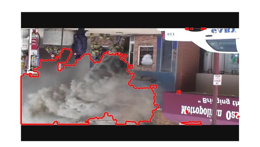
6 CHEN, LI, HALL: MOTION ESTIMATION AND SEGMENTATION OF NATURAL PHENOMENA

                                                      Ours    FullFlow   EpicFlow   Class+NL    HS      BA      LDOF     MDP      FlowNet
                                     Thick_rise       61.60   128.12      166.78     100.03    93.48   100.15   160.14   136.48    135.9
   Our Database

                                Thin_from_bottom      37.89   43.39       43.37      42.44     42.91   42.98    44.08    45.43     39.59
                                 Thin_drops_multi     58.25   73.32       68.12      65.76     67.16   68.33    64.59    68.14     67.03
                                Orange_white_meet     37.89   46.56       41.21      42.14     44.94   43.66    41.75    42.79     42.64
                               Slanted_surface_pour   41.00   59.63       57.73      57.18     56.8    59.58    55.61    56.75     80.11
                                Flat_surface_waves    47.63   48.90       52.17      46.21     44.29   45.30    49.99     50.66    43.37
                                     Steam            7.38      8.84       8.27      12.55     12.52   13.01     12.4    13.57     15.47
                                  Avalanche01         10.43    12.29      12.26      12.12     12.57   12.24    12.78    12.64     17.76
 Public Datasets[12, 17, 32]

                                   Boil (water)       13.27    48.61      18.72      13.91     26.26   25.83    13.94    20.96      42.3
                                   Fountain01         19.69    26.52       18.8      23.67      20.2   20.18    21.39    27.48     22.25
                                   Fountain02         30.67    61.72      31.72      26.93     34.66   25.72     31.3    33.56     27.64
                                   Forest_fire        8.37      8.84       8.39       8.61     10.59   10.45    10.61      9.1     18.85
                                  Landslide01         86.08    87.72      84.94      87.06     89.67   87.82    87.24    86.31     120.2
                                  Landslide02         88.13    86.96      89.43      91.74     89.04   87.49    91.12    91.17     117.7
                               Volcano_eruption01     5.63      5.82       5.99       5.92      6.89    5.98     5.69     5.97      5.63
                               Volcano_eruption02     6.96      7.22       7.41       7.24      7.54    7.47     7.34     7.58      7.5
                                   Waterfall01        17.86     19.1      18.97      21.45      20.8   19.89     19.3     17.9     18.33
                                   Waterfall02        15.8     17.76        18       20.02      17.6   18.32    18.14    18.42     18.89
                                   Waterfall03        13.97    15.06      14.91      18.06     18.14   17.88    16.68    14.82     16.00
                                   Car_smoke          8.85     10.3       10.69      10.64     10.57   10.66    10.58    9.01      10.79
                                   Fire_smoke         12.49    13.21      13.17      12.64     12.81   12.61    12.91    12.68     16.49
  Internet

                                   Avalanche02        12.34    13.36      13.65      13.38     14.05   13.98    14.24    13.95     15.82
                                      Train           11.2     14.13      14.31      14.28     14.18    14.3    14.08    33.44     16.11
                                     Fireman          18.86    19.42      19.42      19.66     19.52   19.56    19.29    20.72     19.04
                                   Match_cube         72.53    74.65      72.93      80.50     87.40   84.32    77.22    87.88     85.09
Table 1: Low Rate Distance (Equation 9) designed for low frame rate video (Public Database
and Internet). We compare our method to eight state-of-the-art algorithms using videos from our
laboratory, from public datasets, and from the Internet; “Train” is a computer graphic simulation.
Bold figures indicate the best performance in each row, we come first in most cases. Data shown
×100 for easy reading. Note that the lower readings show higher accuracy.

used to benchmark general methods. Brox et al. (LDOF) [7] address large motion displacement
issues using feature matching. Xu et al. (MDP) [41] show excellent performance on the Middleburry
benchmark [4]. FlowNet [14] uses a deep neural network and achieves good results. Since the ground
truth motion for natural phenomenon is unavailable we keep the original FlowNet parameters.
   There is no ground truth for any of our video, so we use two measures adapted from the literature.
One measure is similar to in Li et al. [23] who warp frame 1 using the flow, v12, from frame 1 to
frame 2. The warped image is compared to the second frame using mean RMS error. This measure
is suitable for low video frame rates, so we call it the low rate distance (LRD):
                                  LRD=||I2 −warp(I1,v12)||22                                     (9)
 The second measure we used is an adapted version of the Interpolation Error(IE) suggested in [4],
which is better for high frame rate video because it uses frames 1 and 3, tacitly assuming constant
velocity. We compute a forward flow (frame 1 to 3) and a backward flow (frame 3 to 1), then warp
frames 1 and 3, taking the average wherever the flow is consistent, and the forward flow elsewhere.
Again, we use RMS error but now call it high rate distance (HRD):
                       HRD=||I2 −merge[warp(I1,v13),warp(I3,v31)]||22                           (10)

  Results for all videos are shown in Table 1 for LRD, and Table 2 for HRD. The tables show that
our approach consistently outperforms other methods: we come first in most cases. In fact, due to
space limitations, we removed many cases in which were we first; full tables can be found in the
supplementary material. These larger tables show that, on average, our method outperforms all others
by at least 17% when using LRD and 31% when using HRD.
  Figure 3 shows qualitative results which uses a colour wheel to visualise flow. The waterfall
provides a useful example. Our result shows a predominantly downward fall (orange colour), but
captures flow into and away from the fall (cyan) at the top and bottom; these are the cyan regions. All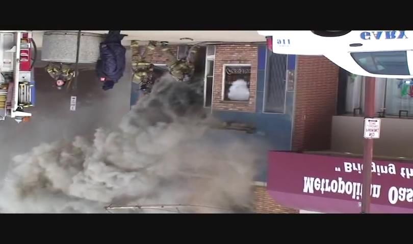
CHEN, LI, HALL: MOTION ESTIMATION AND SEGMENTATION OF NATURAL PHENOMENA 7
Ours FullFlow EpicFlow Class+NL HS BA LDOF MDP FlowNet
Thick_rise 26.74 69.43 72.92 58.54 64.5 53.29 69.16 65.36 61.64
Our Database
Thin_from_bottom 28.03 40.01 41.28 41.32 38.03 40.6 38.95 38.24 30.99
Thin_drops_multi 32.52 44.01 51.35 40.41 43.17 36.3 46.06 40.15 34.37
Orange_white_meet 21.63 34 37.13 37.85 36.88 36.2 33.54 34.98 35.28
Slanted_surface_pour 20.26 44.19 41.94 37.41 34.65 34.75 41.92 41.57 39.81
Flat_surface_waves 16.87 31.55 31.14 30.2 27.96 27.33 30.74 30.88 25.49
Steam 12.51 16.01 15.33 17.40 17.86 16.75 16.36 18.01 18.95
Avalanche01 15.33 28.00 28.53 30.33 27.39 27.58 29.14 28.55 19.75
Public Datasets[12, 17, 32]
Boil_water 35.87 40.37 40.95 36.57 36.62 36.45 39.80 28.55 48.15
Fountain01 36.67 61.69 61.56 50.54 47.68 48.99 50.93 50.68 54.53
Fountain02 137.1 165.4 164.5 235.3 177.1 201.0 164.7 164.7 160.9
Forest_fire 29.81 29.74 31.00 28.27 67.03 78.26 28.66 31.56 26.24
Landslide01 98.01 138.9 142.8 127.2 127.2 129.3 139.1 129.7 142.8
Landslide02 63.17 56.99 66.95 78.93 80.47 57.29 77.23 57.94 58.45
Volcano_eruption01 15.87 21.53 21.43 22.70 21.86 21.69 20.96 21.32 20.65
Volcano_eruption02 13.79 20.23 20.40 20.05 19.50 19.86 19.81 19.32 16.16
Waterfall01 30.78 39.96 40.02 41.38 42.12 45.76 38.76 39.87 42.12
Waterfall02 39.32 35.74 41.78 36.70 37.02 40.39 41.92 39.1 39.69
Waterfall03 34.19 43.06 47.58 42.31 43.80 41.65 42.69 43.08 41.40
Car_smoke 45.26 49.62 50.17 129.6 116.5 114.3 113.6 98.56 101.4
Fire_smoke 60.74 120.5 108.2 52.04 60.98 51.90 53.84 60.56 46.36
Internet
Avalanche02 20.56 29.22 30.98 32.20 23.84 23.48 20.99 20.80 30.45
Train 35.76 83.44 72.45 92.24 91.68 82.13 66.76 150.3 47.11
Fireman 59.84 155.1 167.3 180.8 143.4 180.9 164.9 174.7 124.0
Match_cube 57.59 70.57 71.26 72.75 73.07 72.94 65.23 73.21 73.17
Table 2: High Rate Distance (Equation 10) designed for high frame rate video (our database). We
compare our method to eight state-of-the-art algorithms using videos from our laboratory, from public
datasets, and from the Internet; “Train” is a computer graphic simulation. Bold figures indicate the
best performance in each row, we come first in most cases. Data shown ×100 for easy reading. Note
that the lower readings show higher accuracy.
the alternatives show little other than a strong downward fall. Similar analysis can be applied to the
remaining examples. This paper has space only for qualitative comparison with selected alternatives,
but, our supplementary material holds more sets, where the reader can see the trend persists.
5.2 Segmentation
We compared our results with three segmentation methods. Teney et al. [35] has been designed
expressly to segment dynamic texture and gives excellent results. Papazoglou and Ferrari [27]
is chosen because their approach is fully automatic, and enables to handle unconstrained video.
Segflow[10] provides a very recent comparator.
To obtain a quantitative measure we used a hand-segmented frame as ground truth to compute the
Rand Index [28], which is commonly used for segmentation. We also applied the default parameter
settings for all the baselines and manually select the best result from their outcomes. The reader in
invited to ‘zoom in’ to see details. Results are shown in Table 3. Looking at the results, we see our
method outperforms the state-of-the-art alternatives.
Qualitative results, including the hand-segmentations are shown in 4. These results confirm that
our segmentations are meaningful, but also show that more work is necessary in this problem. Note
that SegFlow [10] proved unable to segment the some phenomena, in those cases we present the
original image.
6 Conclusion and Discussion
We have described a motion estimation algorithm that is robust to a wide range of diverse natural
phenomena, different input video classes at different resolutions and frame rates. Our approach
outperforms state-of-the art methods in most cases. On average, the proposed method is at least 17%
and 31% better than other alternatives based on two evaluation methods. The key to the performance
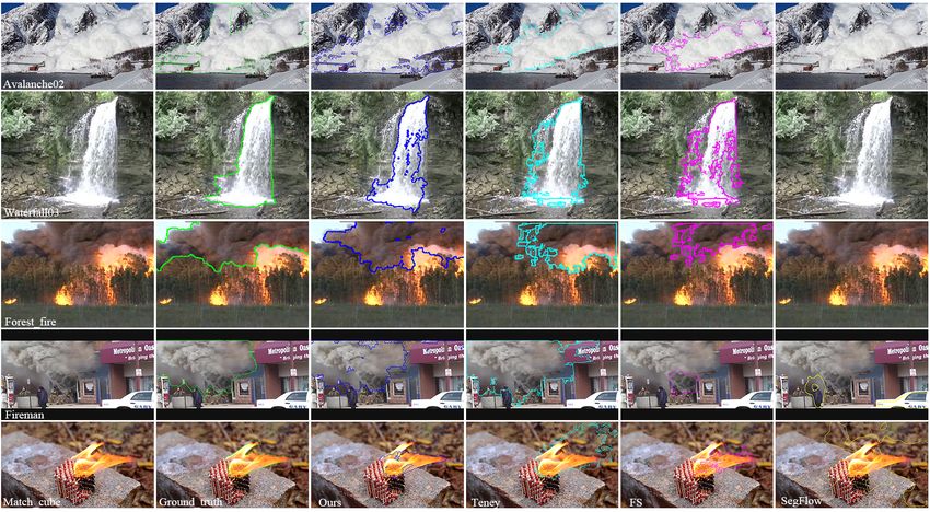
is that we assume global shape changes only a little, which motivates our use of a skeleton as a spatial8 CHEN, LI, HALL: MOTION ESTIMATION AND SEGMENTATION OF NATURAL PHENOMENA Figure 3: Qualitative results for selected phenomena: Left two columns show input frames, subsequent columns show dense flow visualizations for selected contemporary alternatives. From left to right: Ours, FullFlow [31], EpicFlow [29], MDP) [41]. We use colour to indicate direction and magnitude of the flow, see top right for key. Figure 4: Qualitative comparison of segmentations. Left to right: original image; hand drawn ground truth (green); our approach (blue); Teney et al. [35] (cyan); Papazoglou et al.(FS) [27] (magenta); and SegFlow [10] (yellow). Our segmentation yields better representative for the natural phenomena given either clean or complex background. Segflow is able to segment some but not all cases, so some images have no segmentations shown.
CHEN, LI, HALL: MOTION ESTIMATION AND SEGMENTATION OF NATURAL PHENOMENA 9

                                       Ours    Teney [35]    FS [27]   SegFlow [10]
                       Car_smoke       77.78      76.76       68.10        69.11
                       Fire_smoke      89.75      85.46       59.91        51.27
                          Train        94.21      86.41       50.01        56.06
                       Avalanche02     79.49      68.10       57.76        50.20
                       Waterfall03     89.10      86.35       80.72        68.73
                        Forest_fire    82.44      67.10       66.27        57.39
                         Fireman       92.35      89.98       56.64        87.01
                       Match_cube      95.40      81.90       87.89        58.38
Table 3: Average Rand Index (%) evaluation on segmentations for our method and three other
state-of-the-art unsupervised algorithms.

map of topographical features to capture the ‘gist’ of shape, and therefore the ‘gist’ of global flow.
We explain our flow results by posultating that our global, sparse flow we obtain provides a strong
prior constraint for dense, local flow, in the sense of “picking” a useful stating point for search. We
explain our segmentation results by appeal to the diffuse nature of the phenomena we deal with –
particles move freely so that features are highly blurred and transient – our skeleton is robust to such
movements because they change overall shape only a little.
   Like any method, ours has its limitations, each of which provide interesting avenues for future
work. Our motion estimator is designed for natural phenomena rather than, say, articulated objects,
so more general applicability is an open question. A perhaps subtle problem is that we tacitly assume
the spatial distance between skeletal limbs in a single frame exceeds the distance moved by a single
skeletal limb between frames. We have yet to conduct a detailed analysis of this, but preliminary
studies suggest to us there is Nyquist-like problem here that might be solved using a coarse-to-fine
approach over different scales of skeleton. Although we achieve excellent segmentation results, above
state-of-the-art alternatives, it is clear more work needs to be done. We favour an iterative scheme
in which segmentation and motion are jointly estimated. Finally, we have only just begun to explore
the possibilities of using a skeleton for Computer Graphics. Motion editing being the motivation
application is a particular application that would benefit from having a skeleton at hand provides
a mid-level model that could be built into an interactive tool in which users drag skeletons, or even
draw them – but such work is for another paper.
   Our general conclusions from this work are: (i) brightness constancy can and should be replaced
by more appropriate assumptions when needed; (ii) assumptions regarding physical behaviour do not
have to be strong assumptions; and (iii) global behaviour is useful for constraining local behaviour.
7 Acknowledgements
This research is partly funded by CAMERA, the RCUK Centre for the Analysis of Motion, Enter-
tainment Research and Applications, EP/M023281/1.
References
 [1] Radhakrishna Achanta, Appu Shaji, Kevin Smith, Aurelien Lucchi, Pascal Fua, and Sabine Süsstrunk.
     Slic superpixels compared to state-of-the-art superpixel methods. IEEE transactions on pattern analysis
     and machine intelligence, 34(11):2274–2282, 2012.
 [2] Lakshman Anumolu and Imaduddin Ahmed. Simulation of smoke in openfoam framework. 2012.
 [3] Didier Auroux and Jérôme Fehrenbach. Identification of velocity fields for geophysical fluids from a
     sequence of images. Experiments in Fluids, 50(2):313–328, 2011.
 [4] Simon Baker, Daniel Scharstein, JP Lewis, Stefan Roth, Michael J Black, and Richard Szeliski. A database
     and evaluation methodology for optical flow. International Journal of Computer Vision, 92(1):1–31, 2011.
 [5] Frédéric Barbaresco and Bernard Monnier. Rain clouds tracking with radar image processing based
     on morphological skeleton matching. In Image Processing, 2001. Proceedings. 2001 International
     Conference on, volume 1, pages 830–833. IEEE, 2001.
10CHEN, LI, HALL: MOTION ESTIMATION AND SEGMENTATION OF NATURAL PHENOMENA
[6] Michael J Black and Paul Anandan. The robust estimation of multiple motions: Parametric and
piecewise-smooth flow fields. Computer vision and image understanding, 63(1):75–104, 1996.
[7] Thomas Brox and Jitendra Malik. Large displacement optical flow: descriptor matching in variational mo-
tion estimation. Pattern Analysis and Machine Intelligence, IEEE Transactions on, 33(3):500–513, 2011.
[8] Thomas Brox, Andrés Bruhn, Nils Papenberg, and Joachim Weickert. High accuracy optical flow
estimation based on a theory for warping. In Computer Vision-ECCV 2004, pages 25–36. Springer, 2004.
[9] Qifeng Chen and Vladlen Koltun. Full flow: Optical flow estimation by global optimization over regular
grids. arXiv preprint arXiv:1604.03513, 2016.
[10] J. Cheng, Y.-H. Tsai, S. Wang, and M.-H. Yang. Segflow: Joint learning for video object segmentation
and optical flow. In IEEE International Conference on Computer Vision (ICCV), 2017.
[11] Thomas Corpetti, Etienne Mémin, and Patrick Pérez. Estimating fluid optical flow. In Pattern Recognition,
2000. Proceedings. 15th International Conference on, volume 3, pages 1033–1036. IEEE, 2000.
[12] Konstantinos G Derpanis, Matthieu Lecce, Kostas Daniilidis, and Richard P Wildes. Dynamic scene
understanding: The role of orientation features in space and time in scene classification. In Computer
Vision and Pattern Recognition (CVPR), 2012 IEEE Conference on, pages 1306–1313. IEEE, 2012.
[13] Ashish Doshi and Adrian G Bors. Robust processing of optical flow of fluids. Image Processing, IEEE
Transactions on, 19(9):2332–2344, 2010.
[14] Alexey Dosovitskiy, Philipp Fischer, Eddy Ilg, Philip Hausser, Caner Hazirbas, Vladimir Golkov, Patrick
van der Smagt, Daniel Cremers, and Thomas Brox. Flownet: Learning optical flow with convolutional net-
works. In Proceedings of the IEEE International Conference on Computer Vision, pages 2758–2766, 2015.
[15] Ravi Garg, Anastasios Roussos, and Lourdes Agapito. A variational approach to video registration with
subspace constraints. volume 104, pages 286–314. Springer, 2013.
[16] Bernard Ghanem and Narendra Ahuja. Extracting a fluid dynamic texture and the background from
video. In Computer Vision and Pattern Recognition, 2008. CVPR 2008. IEEE Conference on, pages
1–8. IEEE, 2008.
[17] Bernard Ghanem and Narendra Ahuja. Maximum margin distance learning for dynamic texture
recognition. In European Conference on Computer Vision, pages 223–236. Springer, 2010.
[18] James Gregson, Ivo Ihrke, Nils Thuerey, Wolfgang Heidrich, et al. From capture to simulation-connecting
forward and inverse problems in fluids. ACM Transactions on Graphics, 33, 2014.
[19] Berthold K Horn and Brian G Schunck. Determining optical flow. In 1981 Technical Symposium East,
pages 319–331. International Society for Optics and Photonics, 1981.
[20] Yu Ji, Jinwei Ye, and Jingyi Yu. Reconstructing gas flows using light-path approximation. In Computer
Vision and Pattern Recognition (CVPR), 2013 IEEE Conference on, pages 2507–2514. IEEE, 2013.
[21] V Lakshmanan, R Rabin, and V DeBrunner. Multiscale storm identification and forecast. Atmospheric
research, 67:367–380, 2003.
[22] Chuan Li, David Pickup, Thomas Saunders, Darren Cosker, David Marshall, Peter Hall, and Philip Willis.
Water surface modeling from a single viewpoint video. Visualization and Computer Graphics, IEEE
Transactions on, 19(7):1242–1251, 2013.
[23] Feng Li, Liwei Xu, Philippe Guyenne, and Jingyi Yu. Recovering fluid-type motions using navier-stokes
potential flow. In Computer Vision and Pattern Recognition (CVPR), 2010 IEEE Conference on, pages
2448–2455. IEEE, 2010.
[24] Peter Ochs, Jitendra Malik, and Thomas Brox. Segmentation of moving objects by long term video
analysis. IEEE transactions on pattern analysis and machine intelligence, 36(6):1187–1200, 2014.
[25] Abhijit S Ogale, Cornelia Fermuller, and Yiannis Aloimonos. Motion segmentation using occlusions.
IEEE Transactions on Pattern Analysis and Machine Intelligence, 27(6):988–992, 2005.
[26] Makoto Okabe, Ken Anjyo, and Rikio Onai. Extracting fluid from a video for efficient post-production.
In Proceedings of the Digital Production Symposium, pages 53–58. ACM, 2012.
[27] Anestis Papazoglou and Vittorio Ferrari. Fast object segmentation in unconstrained video. In Proceedings
of the IEEE International Conference on Computer Vision, pages 1777–1784, 2013.
[28] W.M. Rand. Objective criteria for the evaluation of clustering methods. Journal of the American Statistical
Association, 66(336):846–850, 1971.
[29] Jerome Revaud, Philippe Weinzaepfel, Zaid Harchaoui, and Cordelia Schmid. Epicflow: Edge-preservingCHEN, LI, HALL: MOTION ESTIMATION AND SEGMENTATION OF NATURAL PHENOMENA 11
interpolation of correspondences for optical flow. In Proceedings of the IEEE Conference on Computer
Vision and Pattern Recognition, pages 1164–1172, 2015.
[30] Hidetomo Sakaino. Fluid motion estimation method based on physical properties of waves. In Computer
Vision and Pattern Recognition, 2008. CVPR 2008. IEEE Conference on, pages 1–8. IEEE, 2008.
[31] Laura Sevilla-Lara, Deqing Sun, Varun Jampani, and Michael J Black. Optical flow with semantic segmen-
tation and localized layers. In IEEE Conference on Computer Vision and Pattern Recognition (CVPR), 2016.
[32] Nitesh Shroff, Pavan Turaga, and Rama Chellappa. Moving vistas: Exploiting motion for describing
scenes. In Computer Vision and Pattern Recognition (CVPR), 2010 IEEE Conference on, pages
1911–1918. IEEE, 2010.
[33] Deqing Sun, Stefan Roth, and Michael J Black. Secrets of optical flow estimation and their principles.
In Computer Vision and Pattern Recognition (CVPR), 2010 IEEE Conference on, pages 2432–2439.
IEEE, 2010.
[34] Damien Teney and Matthew Brown. Segmentation of dynamic scenes with distributions of spatiotemporally
oriented energies. In 25th British Machine Vision Conference, BMVC 2014, 2014.
[35] Damien Teney, Matthew Brown, Dmitry Kit, and Peter Hall. Learning similarity metrics for dynamic
scene segmentation. In Proceedings of the IEEE Conference on Computer Vision and Pattern Recognition,
pages 2084–2093, 2015.
[36] Carlo Tomasi and Roberto Manduchi. Bilateral filtering for gray and color images. In Computer Vision,
1998. Sixth International Conference on, pages 839–846. IEEE, 1998.
[37] Daniel Alejandro Vila, Luiz Augusto Toledo Machado, Henri Laurent, and Ines Velasco. Forecast and
tracking the evolution of cloud clusters (fortracc) using satellite infrared imagery: Methodology and
validation. Weather and Forecasting, 23(2):233–245, 2008.
[38] Guojie Wang, Damien Garcia, Yi Liu, Richard De Jeu, and A Johannes Dolman. A three-dimensional
gap filling method for large geophysical datasets: Application to global satellite soil moisture observations.
Environmental Modelling & Software, 30:139–142, 2012.
[39] Philippe Weinzaepfel, Jerome Revaud, Zaid Harchaoui, and Cordelia Schmid. DeepFlow: Large
displacement optical flow with deep matching. In IEEE Intenational Conference on Computer Vision
(ICCV), Sydney, Australia, December 2013. URL http://hal.inria.fr/hal-00873592.
[40] Chenliang Xu, Caiming Xiong, and Jason J Corso. Streaming hierarchical video segmentation. In
European Conference on Computer Vision, pages 626–639. Springer, 2012.
[41] Li Xu, Jiaya Jia, and Yasuyuki Matsushita. Motion detail preserving optical flow estimation. Pattern
Analysis and Machine Intelligence, IEEE Transactions on, 34(9):1744–1757, 2012.
[42] Tianfan Xue, Michael Rubinstein, Neal Wadhwa, Anat Levin, Fredo Durand, and William T Freeman.
Refraction wiggles for measuring fluid depth and velocity from video. In Computer Vision–ECCV 2014,
pages 767–782. Springer, 2014.You can also read