A Statistical Wisp Model and Pseudophysical Approaches for Interactive Hairstyle Generation
←
→
Page content transcription
If your browser does not render page correctly, please read the page content below
IEEE TRANSACTIONS ON VISUALIZATION AND COMPUTER GRAPHICS, VOL. 11, NO. 2, PP. 160–170, MARCH 2005                                   160

 A Statistical Wisp Model and Pseudophysical Approaches
            for Interactive Hairstyle Generation
                                      Byoungwon Choe and Hyeong-Seok Ko
                                           Seoul National University

Abstract— This paper presents an interactive technique that          gravity and collisions, as well as the variations in hair strands.
produces static hairstyles by generating individual hair strands     This would be labor-intensive and, more importantly, the result
of the desired shape and color, subject to the presence of grav-     would appear unnatural unless the manual creation properly
ity and collisions. A variety of hairstyles can be generated by      conveyed the complexity of real hair.
adjusting the wisp parameters, while the deformation is solved          This paper propose a pseudophysical approach that pro-
efficiently, accounting for the effects of gravity and collisions.   duces realistic hairstyles from a few intuitive parameters and
Wisps are generated employing statistical approaches. As for         provides a means to edit the style in a straightforward way.
hair deformation, we propose a method which is based on              Our method runs fast, thus works interactively; but it does not
physical simulation concepts but is simplified to efficiently        require the users to engage in a cumbersome manual effort. For
solve the static shape of hair. On top of the statistical wisp       example, the effects of gravity and collisions are automatically
model and the deformation solver, a constraint-based styler          generated by the hair deformation solver (Section 3). Varia-
is proposed to model artificial features that oppose the natural     tions among strands are generated using statistical methods
flow of hair under gravity and hair elasticity, such as a hairpin.   (Section 2) that require only a few parameters to be input by
Our technique spans a wider range of human hairstyles than           the users. As a result, our method has a short turnaround time
previously proposed methods, and the styles generated by this        for modeling a hairstyle.
technique are fairly realistic.                                         We note that the framework presented in this paper works in
                                                                     a fashion that is quite simple considering the complexity and
Index Terms— hair modeling, Markov chain, statistical wisp
                                                                     variety of the hairstyles it generates. Rather than applying ad
model, hair deformation solver, hairstyling constraint
                                                                     hoc methods to create different styles, the framework produces
                                                                     various hairstyles by modifying a small number of modeling
1 Introduction                                                       parameters. Still, the synthesized hairstyles are realistic and
                                                                     demonstrate a wide range of hairdos in the real world.

H      AIR constitutes an important part of a person’s overall
       appearance. The same face can make quite different
impressions as the person’s hairstyle is varied. Therefore, to
                                                                     1.1 Related Work
create visually convincing computer-generated humans, it is          In this section, we review the previous work on modeling
imperative to develop techniques for synthesizing realistic hair.    hair geometry, computing hair deformations due to gravity and
   Synthesizing hair requires the modeling, animation, and           collisions, and rendering techniques that can be applied to hair.
rendering techniques. In this paper, we focus on the modeling
aspect. We aim to develop an interactive technique to generate       1.1.1 Modeling Hair Geometry
static human hairstyles in the presence of gravity, with a proper    To model hair by populating a number of strands, the geometry
treatment of collisions.                                             of each individual strand must eventually be modeled. Noting
   Hair strands are very thin (40 to 80 microns in shaft             that adjacent hair strands tend to be alike, Watanabe and
diameter for medium-sized strands [20]) and are subject to           Suenaga [27] introduced a wisp model to generate a group
deformation. Therefore, physically-based methods, such as            of similar neighboring strands by adding variations to one key
finite element analysis or mass-spring simulation, can be            strand. Since then, different methods, such as the thin shell
used to model the shape of a strand in a gravitational field.        volume [12] and the generalized cylinder [29,30], have been
A simple collection of the strands generated by the above            used to represent the wisps. Recently, Kim and Neumann [14]
simulation methods, however, would appear different from             proposed a multi-resolution wisp structure and user interfaces
hair we normally see because hair strands constantly touch           which could model a variety of hairstyles. Ward et al. [26]
or collide with each other; therefore, the interactions among        used level-of-detail representations which modeled individual
strands must be accounted for. Considering that there are            strands and hair clusters with subdivision curves and surfaces,
normally about 100,000 strands of hair [23], the above task          respectively.
would require an enormous amount of computation if only                 The concept of wisp is an important basis of this work.
physically-based methods were used.                                  We also represent wisps using generalized cylinders. However,
   The extreme opposite of the physically-based method would         unlike the previous approaches which model strands and
be to manually control every detail, including the effect of         wisps manually or represent them by parametric functions,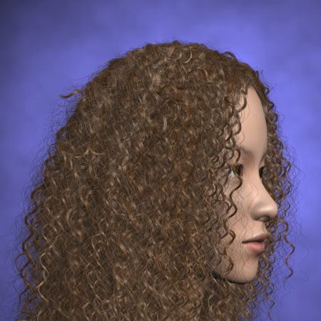
IEEE TRANSACTIONS ON VISUALIZATION AND COMPUTER GRAPHICS, VOL. 11, NO. 2, PP. 160–170, MARCH 2005                                    161

we introduce a statistical wisp model. Starting from a key          1.2 Algorithm Overview
strand, we construct a wisp by duplicating the key strand
                                                                    Our algorithm for hair modeling consists of three steps—
while constraining the wisp shape by some parameters with
                                                                    generating wisps, solving hair deformation, and constraint-
statistical meanings. Moreover, to generate the key strands, we
                                                                    based styling.
introduce a Markov chain hair model by adopting the method
proposed by Hertzmann et al. [10].                                    1. Generating wisps. A whole hair is formed by generating
                                                                         a collection of wisps. We determine the geometrical
   There have been other approaches that do not employ the
                                                                         shape of a wisp by manipulating a representative strand
wisp model. Hadap and Magnenat-Thalmann [8] and Yu [31]
                                                                         and controlling the statistical properties of the surround-
modeled hair as a flow of vector fields and calculated the
                                                                         ing member strands.
strand geometries according to these fields. In simulating dy-
                                                                      2. Solving hair deformation. The hair deformation solver
namic movement of hair, interpolation-based approaches have
                                                                         accounts for the effects of gravity, hair elasticity, and
generally been used [1,5,16,24]: To reduce the computation
                                                                         collisions to determine the deformed shape of the wisps.
required, only a relatively small number of key strands are
                                                                         This procedure is essential for relieving the user of
simulated, and the results are interpolated to generate the
                                                                         excessive manual effort, yet it is flexible enough to
neighboring strands. The above approaches, however, are not
                                                                         handle a wide range of hairstyles.
suitable for modeling non-uniform behavior of human hair
                                                                      3. Constraint-based styling. To model hairstyles such as
such as clustering, which is why we take a wisp-based hair
                                                                         braided hair, we propose a constraint-based approach
model.
                                                                         to make wisps pass through a certain point or follow
   Apart from the above procedural or manual modeling of hair            a certain path. This approach is effective in modeling
geometries, Paris et al. [21] proposed a technique to capture            hairstyles that involve artificial styling pieces such as
hair geometry from multiple images, which showed a new way               hairpins or ribbons.
to generate digital hair.
                                                                    1.3 Paper Organization
1.1.2 Modeling Hair Deformations
                                                                    The remainder of this paper is organized as follows: Sections
Deformations due to gravity and collisions can be dealt with by     2, 3, and 4 present the statistical wisp model, the hair de-
employing physically-based models such as a simplified can-         formation solver, and the constraint-based styler, respectively;
tilever beam model [1,16], a mass-spring-hinge model [5,24],        Section 5 describes how rendering is implemented; Section 6
or a combination of a multi-body serial chain and a continuum       summarizes experimental results; and Section 7 concludes the
hair model [9]. Extensions to the above models to allow for the     paper.
use of the wisp structure have also been proposed [3,4,22,25].
However, those methods were targeted for animating hair of
some limited styles, thus were not suitable for generating a
                                                                    2 Statistical Wisp Model
variety of static hairstyles. Therefore, in the systems dedicated   It is readily observable that hair exhibits clustering behavior; a
to modeling complicated hairstyles [14,29,30], the deformed         group of hair strands that are spatially close and geometrically
hair shapes have been created manually.                             similar is called a wisp. We view the task of synthesizing
   In this work, we propose a new hair deformation solver           a hairstyle as generating a collection of wisps. This section
which is different from the previous approaches: It is tailored     describes how we generate the hair strands and wisps by
to handle static hairstyles and automatically generates the         controlling the statistical properties of hair.
shape of hair that has been deformed due to the effects of
gravity and collisions. The method is based on the physical         2.1 Wisp Modeling
principles involved in hair deformation, but is simplified to
solve only static hair shapes.                                      Our wisp model consists of a master strand and numerous
                                                                    member strands, and the overall shape of the wisp is a gen-
                                                                    eralized cylinder. This section describes the wisp generation
1.1.3 Rendering Hair
                                                                    algorithm under the assumption that the geometry of the
To render a hair strand, Kajiya and Kay’s reflectance model         master strand is given; the method for generating the master
[7,11] has been widely used; we also use this model in this         strand is presented in Section 2.2.
work. Lately, Marschner et al. [19] measured the scattering            We represent a strand as a Catmull-Rom spline, which is
from real individual hair fibers and proposed a shading model       defined by and passes through a sequence of control points
to render complicated scattering effects based on these ob-         {p1 , p2 , · · · , pn }. The spline p(s) is parameterized within the
servations. To account for self-shadowing among hair strands,       range [0, 1] so that p(0) = p1 and p(1) = pn correspond to the
LeBlanc et al. [15] proposed a method that uses pixel blending      root and tip of the strand, respectively.
and shadow buffers. The deep shadow map proposed by                    Within a wisp, the degree of similarity among the strands
Lokovic and Veach [18] extended the concept of a conven-            is controlled by the length distribution, the deviation radius
tional shadow map to cover volumetric objects such as smoke         function, and the strand-shape fuzziness value.
and hair. Kim and Neumann [13] showed that the deep shadow             • Length distribution l(u) is a probability density function
map can be implemented efficiently on graphics hardware.                  that gives the probability that a member strand will have
IEEE TRANSACTIONS ON VISUALIZATION AND COMPUTER GRAPHICS, VOL. 11, NO. 2, PP. 160–170, MARCH 2005                                                          162

    l                                l                                 r                     r
                                                                                            2.0

                       u                                 u
                                                                      1.0
                                                                      0.5             s
                                                                                           1.0
                                                                                                           s             σ = 0.1               σ =1
                 1.0                               1.0                          1.0                  1.0

Fig. 1.   Wisps generated by two different                         Fig. 2.   Wisps generated by two different      Fig. 3.   Wisps generated by two different
length distributions.                                              deviation radius functions.                     fuzziness values.

     length u, relative to the length of the master strand                                where rk−1 and rk are the deviation radii at pk−1 and pk ,
     (Fig. 1).                                                                            respectively, and e is a three-dimensional noise vector.
  • Deviation radius function r(s) specifies an upper limit                                  The vector e cannot have an arbitrary value because dk must
     on the positional offset of the member strands from the                              lie within the sphere of radius rk according to the definition of
     master strand at the parameter value s; it controls the                              the deviation radius function. Let the noise vector be expressed
     shape of the generalized cylinder representing the wisp                              as e = yx̄, where x̄ is a unit direction vector and y is a scalar
     (Fig. 2).                                                                            value. To determine the noise vector e:
  • Strand-shape fuzziness value σ controls the variation                                    1. x̄ is randomly selected;
     of the strands within a wisp. Fig. 3 shows the appearance                               2. y is randomly chosen while |dk | < rk is satisfied.
     of wisps at σ = 0.1 (low variance) and σ = 1 (high                                   To find y, a ray is cast originating from pO            M    rk
                                                                                                                                           k = pk + rk−1 dk−1
     variance).
                                                                                          in the direction of x̄ until the ray intersects the sphere at a
  Now, the member strands are formed from the master strand                               point pSk . Let L be the distance from pO             S
                                                                                                                                         k to pk . A value for
by applying l(u), r(s) and σ . The k-th control point pk of a                             y is then chosen from the uniform distribution of the range
member strand is computed by adding a displacement dk to                                  [0, min(L, σ · rk )] as illustrated in Fig. 4. Therefore, dk remains
the k-th control point pM
                        k of the master strand:                                           within the sphere, and the control points of the member strands
                                         pk = pM                                          are not concentrated at the boundary of the sphere.
                                               k + dk .
                                                                                             The above procedure is repeated until the member strand
Assuming that the displacement at the root d1 = p1 − pM1                                  attains the desired length u relative to the master strand.
is known, dk is computed iteratively using the following
equation:
                          rk                                                              2.2 Master Strand Modeling
                   dk =       dk−1 + e,              (1)
                         rk−1                                                             The wisp modeling algorithm assumes that the master strands
                                                                                          have been already given. This section presents how we actually
                                                                                          model the geometry of a master strand.
          p Sk             pk                                                                It is generally accepted that hair strands from a single person
                                    pO                                                    resemble each other, which forms a unique characteristic of
                  e= yx              k
                                                                                          the person’s hairstyle. In our wisp model, an effective way of
                                     rk                      r
                                                             k
                                         dk −1 p M                                        ensuring that the entire hair possesses a common pattern is to
                                    rk−1         k
                                                                                          enforce that all the master strands have the same pattern. Then
                                                                                          the member strand generation algorithm (Section 2.1) extends
                           p k −1                            r
                                                             k−1                          this pattern to the entire hair.
                                         dk −1
                                                 p kM−1                                      We obtain the master strands of a common pattern by
                                                                                          synthesizing new strands that resemble a given prototype
                                                                                          strand. To synthesize a new similar strand from the prototype,
                                     master strand                                        we adopt the example-based Markov chain models [6,10,28],
Fig. 4. Computing the point pk of a member strand from the points                         but formulate it as a Gibbs distribution to mathematically
pM      M                                                                                 control the degree of similarity between the prototype and the
 k and pk−1 of the master strand.
                                                                                          synthesized strand.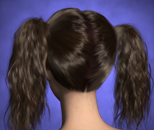
IEEE TRANSACTIONS ON VISUALIZATION AND COMPUTER GRAPHICS, VOL. 11, NO. 2, PP. 160–170, MARCH 2005 163
outline
detaili+2 joint i+2
detaili+1 joint i+1
joint i detaili
(a) (b)
Fig. 5. Representation of the master strand: (a) the original curve,
(b) the outline and details components.
2.2.1 Strand Representation
Instead of directly manipulating the control points
{p1 , p2 , · · · , pn } of a master strand, we decompose them into an
outline component, {c1 , c2 , · · · , cn }, and a details component, Fig. 6. Synthesizing a new strand from a prototype: To find δi ,
{δ1 , δ2 , · · · , δn }, such that pi = ci + δi (i = 1, 2, · · · , n). In the window ω (δi ) is compared with every possible window in the
Fig. 5 (b), the straight line segments at the center correspond prototype, then δk∗ is selected from the prototype based on Eq. (4).
to the outline component of the strand; they are connected
with 3-DOF rotary joints, and ci represents the position of
the joint center. We use the segments of the equal length
neighborhood containing only the points preceding the current
between the joints to simplify the calculation of deformations
point. Therefore, in the sequence of the details component
in Section 3. The displacements from the joint centers to the
{δ1 , δ2 , · · · , δn }, the neighborhood of δi is defined by
control points correspond to the details component.
The purpose of the decomposition is to separate the intrinsic
ω (δi ) = {δi−h , δi−h+1 , · · · , δi−1 },
geometry of the strand from the deformations applied to it by
styling procedures. The subsequent deformations of the strand
where h is the window size.
modify only the joint angles of the outline component, but
Let ε (ωi , ω j ) be the Euclidean distance between the two
do not modify the details component. As a consequence, the
h-sized windows ω (δi ) and ω (δj ):
geometrical characteristics—which are encoded by the details
component—can be preserved. v
u h
u ¯ ¯2
2.2.2 Strand Synthesis ε (ωi , ω j ) = t ∑ ¯δi−t − δj−t ¯ . (2)
t=1
The outline component of the strand consists of straight
line segments, thus is determined straightforwardly once the
segment length Ls is given. This section describes how the Now, the problem of determining δi so that ω (δi ) resembles
details component is generated from a prototype strand. the prototype pattern can be reduced to finding a portion
The control points of a new strand must be established so ω (δk∗ ) = {δk−h
∗ ,δ∗
k−h+1 , · · · , δk−1 } of the prototype strand such
∗
that the strand resembles the given prototype. Assuming that that
a hair strand can be modeled as a Markov chain, we can min{ε (ωi , ωk∗ )}. (3)
k
construct the details component by sequentially determining
δi (i = 1, 2, · · · , n) until the curve has reached the desired Then we can deterministically specify δi to be δi = δk∗ .
length while observing only the neighborhood of δi . Let
However, the diversity of synthesized strands can be in-
{δ1∗ , δ2∗ , · · · , δm∗ } be the details component of the prototype
creased by stochastically selecting the details component in-
strand. To determine δi , we examine the prototype strand and
stead of the optimal choice given by Eq. (3). We introduce
find the best match δk∗ while restricting the comparison only
the Gibbs distribution as a selection probability Pk for each
to the neighborhood of δi as illustrated in Fig. 6.1
possible window of the prototype strand:
The neighborhood is modeled as a window—a set of control
µ 
points—around the current control point. Intuitively, the size 1 ε (ωi , ωk∗ )
of the window should be on the scale of the largest regular Pk = exp − , (4)
Z T
structure of the curve; otherwise, the structure may be lost.
We also let the neighborhood be causal: We construct the where T is the temperature of the system, which can be
1 We adopt an approach similar to that used in “curve analogy” [10], which
controlled by the
¡ user, and Z ¢is the partition function defined
can be referenced for the detailed description of the curve synthesis algorithms by Z = ∑k exp −ε (ωi , ωk∗ )/T . The strand diversity increases
using Markov chains. as T increases, which is demonstrated in Fig. 7.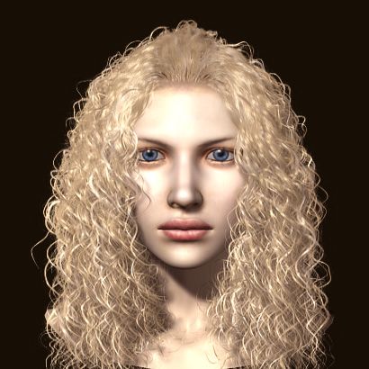
IEEE TRANSACTIONS ON VISUALIZATION AND COMPUTER GRAPHICS, VOL. 11, NO. 2, PP. 160–170, MARCH 2005                                      164

                                                                         mine the length and protrusion direction of the master strands.
                                                                         For the member strands, these properties are determined by the
                                                                         algorithm presented in Section 2.1.

                                                                         3 Hair Deformation Solver
                                                                         In this section, we address the problem of determining the
                                                                         shape of wisps under the influence of gravity and collisions.
                                                                         The purpose of the hair deformation solver is to find the joint
                                                                         angles of the master strands after these factors are taken into
                                                                         account. Then the shape of the member strands is routinely
                                                                         determined from the shape of the master strand (Section 2.1).
     (a)              (b)          (c)          (d)          (e)            Our hair deformation solver is based on two ideas. Firstly,
Fig. 7. The effects of T on the master strand shape: (a) the prototype   it incorporates the physical properties of hair, but avoids
strand and synthesized strands when (b) T = 0.01, (c) T = 0.03, (d)      dynamics simulation. Styling operations such as braiding
T = 0.07, (e) T = 0.12.                                                  assemble hair into a complex structure that is beyond the
                                                                         realm of simple Newtonian mechanics. Instead of simulating
                                                                         those situations in a pure physically-based way, we deal with
                                                                         gravity and the current styling operation as a unified force
2.3 Global Hair Parameters                                               field, and solve the deformation employing pseudophysical
At the topmost level, the user sets the number of wisps Nw and           approaches. Secondly, the deformation solver models hair as
the total number of hair strands Ns . The user then interactively        a continuum, as proposed by Hadap and Magnenat-Thalmann
constructs the density, length, and protrusion maps which                [9], and interprets density as a measure of collision. When the
define the corresponding hair properties for every point in the          density of a certain region is above a threshold, it is regarded
scalp region. The effects of the density and length maps are             as a collision and the hair is forced to occupy a larger volume.
illustrated in Fig. 8.                                                      We implement the two ideas within a single framework.
   Once Nw is given, the root positions of the master strands are        The deformation solver works quickly, and can be applied to
determined by evenly distributing the number of points over              a wide range of hairstyles.
the scalp region. Voronoi diagrams can then be generated to
set the boundary of each wisp. Finally, using the density map            3.1 Deformation Due to Styling Force Field
and Ns , the roots of the member strands are randomly located
                                                                         The styling force field Φ(x), defined in 3D space, quantitatively
within each Voronoi region.
                                                                         combines the effects of gravity and styling operations to
   Note that the length and protrusion maps are used to deter-
                                                                         represent the desired flow direction and intensity at each 3D
                                                                         point x. The force fields rotate the joint so that the outline
                                                                         segment (Figure 5) attached to the joint is oriented along
                                                                         Φ(x). However, hair has an elastic property that resists such
                                                                         deformation in proportion to the bending amount and stiffness.
                                                                         Therefore, we determine the orientation of a segment by
                                                                         finding the joint angle that maximizes the following equation:
                                                                                                 E = EΦ + κ EB ,                      (5)
                                                                         where EΦ represents the degree to which the strand is aligned
                                                                         with the force field, and EB represents the degree to which the
                                                                         strand is aligned with its rest position.
                                                                            Let q be the unit direction vector of the segment. EΦ is
                                                                         calculated by the following function:
                                                                                                 EΦ = Φ(x) · q,
                                                                         and its value is greatest when q is aligned with Φ(x). EB
                                                                         represents the (inversely proportional) amount of bending by
                (a)                               (b)
                                                                                                   EB = q0 · q,
Fig. 8.    Density and length maps and their effects: (a) a density
map (top)—with bright area representing high density and dark area       where q0 is the direction of the segment when the joint
representing low density—and its effect on hair (bottom), (b) a length   angle is zero. Finally, κ is the scalar value that models the
map (top)—with bright area representing long hair and dark area
representing short hair—and its effect on hair (bottom).                 bending stiffness of hair. Fig. 9 (a) and (b) show the resulting
                                                                         deformation for two different values of κ .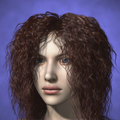
IEEE TRANSACTIONS ON VISUALIZATION AND COMPUTER GRAPHICS, VOL. 11, NO. 2, PP. 160–170, MARCH 2005                                                   165

                                                                                 for τ , the overall hair volume becomes larger, as demonstrated
                                                                                 in Fig. 9 (c).

                                                                                 3.3 Implementation Using a 3D Grid Structure
                                                                                 The description of the previous two sections was based on
                                                                                 continuous fields. To implement the algorithms in a discretized
                                                                                 space, a three-dimensional grid is constructed around the
                                                       (b)                       head and shoulder that includes all regions where hair may
                                                                                 potentially be placed during the styling process. The values of
                                                                                 the styling force and density are then stored only for points on
                                                                                 the grid. The styling force and density at an arbitrary point in
                   (a)                                                           the 3D space is obtained by performing a trilinear interpolation
                                                                                 of the values at the eight nearest grid points.
                                                                                    The hair deformation solver works by repeating the follow-
                                                                                 ing two steps: (1) Deform the strands based on the fields,
                                                       (c)                       and (2) update the density field based on the deformation.
                                                                                 One question remains: whether the steps should run in the
Fig. 9.    Effects of bending stiffness κ and density threshold τ on             breadth-first order or depth-first order. We choose the breadth-
hairstyles: (a) κ = 0.5, τ = 0.9; (b) κ = 2.5, τ = 0.9; (c) κ = 0.5,
                                                                                 first order with the rationale that this handles hair-to-hair
τ = 0.1.
                                                                                 collisions better than the depth-first order does, especially
                                                                                 because the master strands have the segments of the equal
                                                                                 length (Section 2). We summarize the procedure for the hair
   Since the optimization function in Eq. (5) is linear, it can                  deformation solver in Algorithm 1.
be easily solved to find the unit vector q∗ that maximizes it.
The joint angle corresponding to q∗ can then be calculated
                                                                                 Algorithm 1 Hair deformation solver
straightforwardly.
                                                                                   initializeDensityField(); // 1 inside and 0 outside the head
   The above procedure determines the angle for a single                           for joint = 1 to J /* root-to-tip order */ do
joint. To determine the shape of an entire master strand, the                         for wisp = 1 to W do
procedure is repeated along the strand, from the root to the                             deformByStylingForceField(); /* Eq. (5) */
tip.                                                                                     for grid points occupied by the wisp segment do
                                                                                            while checkCollision() /* Eq. (6) */ do
                                                                                              bend the joint by ∆θ along the density gradient;
3.2 Deformation Due to Density Field                                                        end while
                                                                                         end for
We now account for the hair-to-head and hair-to-hair col-                                updateDensityField(); // add the density of this segment
lisions. Detecting collisions between every pair of strands                           end for
would be computationally intractable. Fortunately, when we                         end for
observe a hairstyle, collisions between individual strands are
not noticeable. When wisps cross each other, however, it
produces unmistakable artifacts. Therefore, our collision res-
olution method is developed to handle collisions at the wisp                     4 Constraint-Based Styler
level.
   We interpret that hair produces a density field.2 When the                    The hair deformation solver is quite powerful in producing
procedure in Section 3.1 would locate a wisp segment in                          the styles that are based on the natural flow of hair under
a position x, it is first checked whether the wisp segment                       the gravity field. However, the method is not easily applicable
introduces a collision by:                                                       to producing artificial hairstyles such as braids. To produce
                                                                                 such types of hairstyles, we take a new approach—styling
                           ρ (x) + ρ∆ (x) > τ ,                           (6)    constraints.
where ρ (x) is the existing density value at x, ρ∆ (x) is the                       A constraint causes a constraint force field Ψ(x) to be
increased density that would be added due to the positioning                     generated over a portion of the 3D space, as shown in Fig. 10.
of the wisp segment, and τ is the density threshold. When the                    When and only when the hair deformation solver processes the
sum on the left-hand side of Eq. (6) is greater than τ , this is                 portion being constrained, instead of the original styling force
treated as a collision and the segment is reoriented based on                    field Φ(x), it uses a modified styling force field Φ0 (x) given
the gradient of the density field. When a small value is used                    by
                                                                                                  Φ0 (x) = (1 − w)Φ(x) + wΨ(x),               (7)
   2 Even though the geometries of the strands are defined after the wisps are
generated (Section 2), the strands are regarded as not existing yet. When the    where the control parameter w is the weight of the constraint
hair deformation solver starts processing strands, the density over the entire
space is zero. Once the solver calculates a segment, the density corresponding   force field Ψ(x) relative to the original styling force field Φ(x).
to the segment is created.                                                       Other than the selective superimposition of the constraint force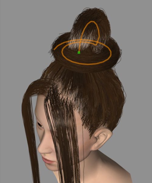
IEEE TRANSACTIONS ON VISUALIZATION AND COMPUTER GRAPHICS, VOL. 11, NO. 2, PP. 160–170, MARCH 2005                                             166

                                                                                 apply to the selected portion.
                                                                              When the hair deformation solver processes those selected
                                                                           wisps, the constraint force field Ψ(x) is superimposed with the
                                                                           styling force field Φ(x). The constraint-based styler activates
                                                                           the first constraint in the queue and processes the selected
          (a)                     (b)                    (c)               wisps until they all meet the constraint. It then processes
                                                                           each subsequent constraint, one at a time, in the queue.
Fig. 10. Three styling constraints: (a) point constraint, (b) trajectory   When all of the constraints have been processed, the hair
constraint, (c) direction constraint.
                                                                           deformation solver resumes processing the wisps in the usual
                                                                           way. Figure 11 demonstrates the use of two different constraint
                                                                           queues.
field over the original styling force field, the hair deformation
solver works in the same way.
   Based on the results of our experiments, we have concluded
that the three types of styling constraints illustrated in Fig. 10         5 Rendering
can be used to create most of the artificial hairstyles.
   • Point Constraint: A point constraint is specified by an               The geometric models of hair would not look natural unless
      attraction point and a tolerance radius. This constraint             they are rendered properly. Rendering quality is more impor-
      produces vector fields toward the attraction point, as               tant for hair than other parts of the body. This section addresses
      shown in Fig. 10 (a). The constraint force vector is                 two problems: how to determine the colors of individual
      activated only until the wisp comes within the sphere.               strands, and how to render the hair geometries.
   • Trajectory Constraint: A trajectory constraint is speci-                 The colors of strands taken from the same person might
      fied by a trajectory and a tolerance radius. The constraint          appear to be similar. However, closer examination reveals
      generates unit vectors (1) toward the nearest point of               that no two hair strands have exactly the same color. To
      the trajectory for grid points lying outside the tolerance           modulate the change of hair colors, a stochastic approach
      radius, or (2) in the tangential direction of the trajectory         is employed. We adopt HSV color space, and model hue,
      for grid points lying inside the tolerance radius, as shown          saturation and value (brightness) channels as three independent
      in Fig. 10 (b).                                                      probability density functions, using either uniform or Gaussian
   • Direction Constraint: A direction constraint is specified             distributions. The different effects produced by adopting these
      by a trajectory and an influence radius. For grid points             two distributions are shown in Fig. 12 (b) and (c). We can
      lying within the influence radius, the constraint generates          also control the color variations at the wisp level, as shown in
      unit vectors in the tangential direction of the trajectory,          Fig. 12 (d).
      as shown in Fig. 10 (c).
                                                                              In order to explicitly render individual hair strands, the
   The functioning of the constraint-based styler can be sum-              Catmull-Rom splines, representing the strands (Section 2), are
marized as follows:                                                        converted to thin ribbons using the RiCurves primitive in
   1. Select the portion of hair, consisting of a set of wisps,            RenderManT M [2]. Then the hair shading model proposed
        upon which to apply the constraints.                               by Kajiya and Kay [11] is used for shading each strand.
   2. Build a constraint queue, a sequence of constraints, to              Finally, the deep shadow map [18] is used to represent the self-
                                                                           shadowing among hair strands, which is essential for creating
                                                                           the volumetric appearance of hair.

                 (a)                               (b)                            (a)              (b)               (c)              (d)
Fig. 11. Examples of using the constraint-based styler: (a) applying       Fig. 12. Hair color corresponding to different probability dis-
a single [point + trajectory] constraint queue to a group of hair, (b)     tributions: (a) constant color, (b) uniform distribution, (c) Gaussian
applying three [point + trajectory] constraint queues to three groups      distribution, (d) variation of colors in the wisp level.
of hair, respectively. Fig. 15 (c) and (d) show the rendered images of
these hairstyles.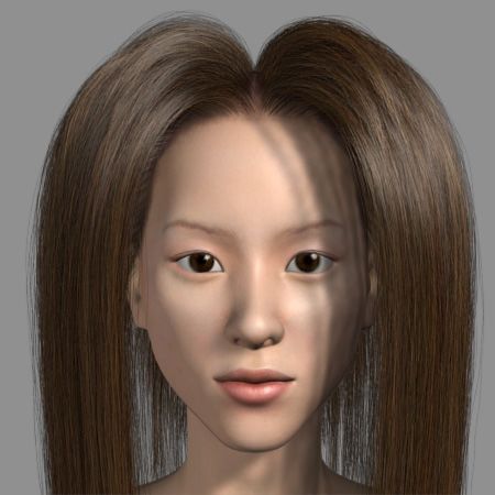
IEEE TRANSACTIONS ON VISUALIZATION AND COMPUTER GRAPHICS, VOL. 11, NO. 2, PP. 160–170, MARCH 2005 167
Fig. 13. Hairstyles produced by applying the statistical wisp model and the hair deformation solver. Each hairstyle has approximately
80,000 to 100,000 strands.
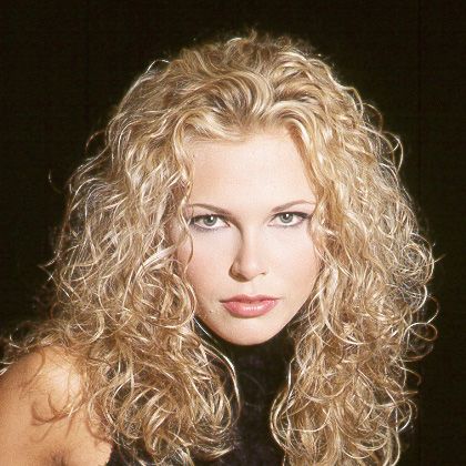
(a) (b) (c) (d)
Fig. 14. Synthetic hairstyles inspired by real ones: (a) a real hairstyle and (b) a corresponding synthetic one generated by applying the
statistical wisp model and hair deformation solver; (c) a real updo hairstyle and (d) a synthetic imitation of it obtained by applying the
constraint-based styler (images by the courtesy of http://www.hairboutique.com).
6 Results and the number of strands Ns .
3. Edit the geometry of the prototype strand: The user
We implemented the presented techniques on a PC with an models the prototype strand with a 3D spline curve.3
Intel Pentium (4) 2.54GHz CPU and an NVIDIA GeForce FX 4. Tune the wisp parameters—the length distribution l(u),
5600 GPU. To check the intermediate results during styling deviation radius function r(s), and fuzziness value σ .
processes, we also implemented a renderer on a programmable 5. Setup the styling force field (see Section 6.1 for the
graphics hardware [17]. details).
Using our hair modeling system, both ordinary users 6. Tune the deformation parameters—the bending stiffness
and professional hairstylists were asked to either reproduce κ and the density threshold τ .
hairstyles from beauty magazines or to create novel hairstyles. 7. Specify the hair color: When the user uses the Gaussian
To help the readers understand how the whole system works, color model, he/she inputs the mean and variance of
we summarize the steps taken for the hairstyling. The user three HSV channels.
starts the styling work on a given 3D polygon model of head
Fig. 13 shows some hairstyles created by taking the above
and shoulder. In a preprocessing step, the scalp surface is
modeling steps. Approximately 80,000 to 100,000 hair strands
specified as a polygonal surface, which defines the region
were used for generating each hairstyle. The computation time
where hair follicles exist. Then, the following steps are taken:
1. Construct the density, length, and protrusion maps. 3 We also provided pre-modeled samples representing the various types of
2. Tune the global parameters—the number of wisps Nw curly and wavy hair so that the user could simply select one from the samples.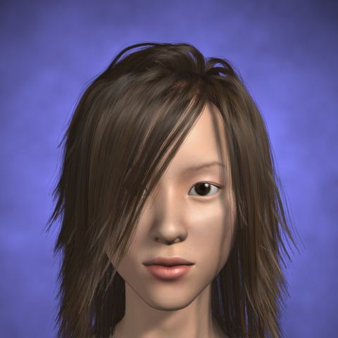
IEEE TRANSACTIONS ON VISUALIZATION AND COMPUTER GRAPHICS, VOL. 11, NO. 2, PP. 160–170, MARCH 2005                                         168

                      (a)

                                                                   (c)

                      (b)                                                                                        (d)
Fig. 15.    Hairstyles produced by the constraint-based styler after applying (a) a single point constraint, (b) two point constraints, (c) a
point constraint followed by a trajectory constraint, (d) three sets of a point constraint followed by a trajectory constraint.

greatly depended on the number of control points in a strand as          only for the rough-level control of a hairstyle. The detailed
well as Nw and Ns . In the initial setup, most time was spent on         properties of hair depend on separate controls. Preventing the
user interactions for preparing input to the system. However,            penetration of hair into the head is done by the collision
once the input was provided, usually the result could be seen in         resolution procedure (Section 3.2). Geometric details of hair
less than 10 seconds on the hardware renderer which rendered             strands are generated inside the wisp model (Section 2).
about 20,000 strands. The accompanying video shows, step by              Therefore, even though the current procedural construction
step, how the above modeling procedure is done.                          is not an ultimate interface for specifying the force fields in
   When a desired hairstyle was formed after tuning the                  general, it already provides enough flexibility to generate the
parameters, it finally went through a software renderer, which           variety of hairstyles in Fig. 13.
produced the results shown in Fig. 13. The software rendering
took about 30 minutes to render a hairstyle. Fig. 14 shows real          6.2 Hairdressing Operations
hairstyles and the corresponding synthetic imitations modeled
after the real ones.                                                     Since the five hairdressing operations—cutting, permanent
                                                                         waving, combing, tying, and braiding—would produce most
                                                                         human hairstyles, showing that our modeling system is capable
6.1 Producing Styling Force Field                                        of implementing these operations can give an estimation of the
Currently, we construct the styling force field using a procedu-         applicable range of the proposed technique.
ral approach. For convenience, we provide the users predefined              • Cutting: It can be implemented by directly editing the
force fields—e.g., gravity field, pulled-back hair field. To allow            length map.
general users to fully exploit our system, a tool for editing               • Permanent waving: It can be achieved by giving a
vector fields, such as the one described in [8], should be                    prototype strand of the desired shape to the statistical
implemented in the future.                                                    wisp model.
   It needs to be noted that our use of vector field is somewhat            • Combing: It can be implemented using a direction con-
different from that in the previous work [8,31], where almost                 straint. First, a portion of hair is selected for combing,
all the aspects of hairstyles are directly controlled by the                  then the desired trajectory is indicated. Finally, we specify
vector field. For instance, the vector field should be carefully              the weight w of Eq. (7) that controls the influence of the
constructed to prevent the penetration of hair into head. The                 constraint force field relative to the styling force field.
strand details are also controlled by the vector field: e.g., curly         • Tying: The portion to tie is selected, and a point con-
hair is generated by applying perturbations to the vector field.              straint is imposed so that the selected portion is attracted
   On the other hand, the construction of the force field in                  to the point. A value of w = 1 is used so that the portion
our system is much less cumbersome since the field is used                    is entirely affected by the constraint force field. Once the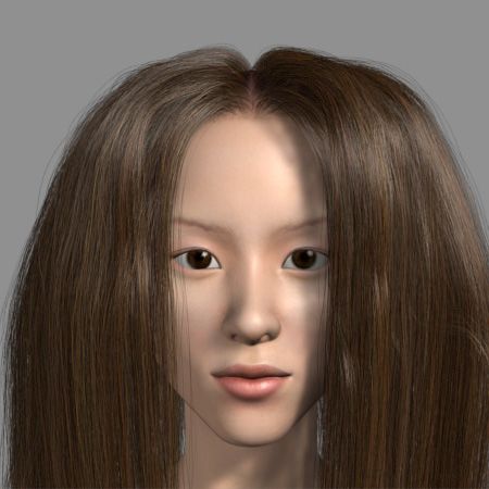
IEEE TRANSACTIONS ON VISUALIZATION AND COMPUTER GRAPHICS, VOL. 11, NO. 2, PP. 160–170, MARCH 2005                                              169

      constraint is met, the selected portion is then affected by     Limitations and Future Work: The dynamic movement of
      the normal styling force field.                                 hair is not considered in this work, though the technique is
  •   Braiding: It can be implemented by applying a point             still useful for many applications. Hair, especially short hair,
      constraint followed by a trajectory constraint to three         generally moves very little unless there is a strong wind or the
      or more groups of hair. Each group of strands is first          character makes a sudden movement; as a result, the technique
      gathered at the point specified by the point constraint.        can be used in some limited cases of character animation.
      Then the trajectory constraint is applied so that the strands   As future work, we are developing hair simulation technique
      form braids.                                                    based on the wisp models presented in this paper. Another
   Fig. 15 demonstrates several hairstyles produced by ap-            limitation of this work is the difficulty of modeling hairstyles
plying these operations. All hairstyles commonly involved             where the wisps are closely packed so that there are too many
cutting, permanent waving and combing. We additionally                collisions among them. To solve this problem, we could use
applied tying operations to produce the styles in Fig. 15 (a) and     a multi-resolution approach such as the “wisp tree” [3,14].
(b), a variation of the tying operation followed by a trajectory
constraint for an updo style in Fig. 15 (c), and the braiding         Acknowledgments
operation for Fig. 15 (d). In the production, the accessories,
such as a ribbon, did not affect the styling, but were added          This research was supported by the Ministry of Information
just to enhance the visual realism. The accompanying video            and Communication, Republic of Korea. This work was also
shows the user interface for hairdressing operations.                 partially supported by the Automation and Systems Research
                                                                      Institute at Seoul National University and the Brain Korea 21
                                                                      Project. The authors would like to thank Prof. Il Dong Yun for
7 Conclusion                                                          his inspiration and guidance at the initial stage of this research.

We have presented a technique for interactively modeling
human hair. A variety of hairstyles can be generated by
                                                                      References
modifying a small number of wisp parameters while the effect           [1] K. Anjyo, Y. Usami, and T. Kurihara. A simple method for extracting
of gravity is automatically solved by the hair deformation                 the natural beauty of hair. In Computer Graphics (Proceedings of
                                                                           SIGGRAPH 92), volume 26, pages 111–120, July 1992.
solver. The framework is quite versatile to be capable of              [2] A. A. Apodaca and L. Gritz. Advanced RenderMan: Creating CGI for
realizing familiar but non-trivial styling operations such as              Motion Pictures. Morgan Kaufmann, 1999.
permanent waving and braiding in a straightforward manner.             [3] F. Bertails, T. Kim, M.-P. Cani, and U. Neumann. Adaptive wisp tree -
The technique provides improvements over previous methods                  a multiresolution control structure for simulating dynamic clustering in
                                                                           hair motion. In ACM SIGGRAPH Symposium on Computer Animation,
in the reality of the result and the range of hairstyles it can            pages 207–213, 2003.
produce.                                                               [4] J. T. Chang, J. Jin, and Y. Yu. A practical model for hair mutual
                                                                           interactions. In ACM SIGGRAPH Symposium on Computer Animation,
   The speedup, realism, and diversity are possible due to the             pages 73–80, July 2002.
combination of the statistical wisp model, the hair deformation        [5] A. Daldegan, N. M. Thalmann, T. Kurihara, and D. Thalmann. An
solver, the constraint-based styler, and the stochastic hair color         integrated system for modeling, animating and rendering hair. Computer
                                                                           Graphics Forum (Eurographics ‘93), 12(3):211–221, 1993.
model.                                                                 [6] A. A. Efros and T. K. Leung. Texture synthesis by non-parametric
   Firstly, the statistical wisp model has relieved us from                sampling. In IEEE International Conference on Computer Vision, pages
modeling each hair strand manually or by employing paramet-                1033–1038, Sept. 1999.
                                                                       [7] D. B. Goldman. Fake fur rendering. In Proceedings of SIGGRAPH
ric functions. We have introduced an example-based Markov                  97, Computer Graphics Proceedings, Annual Conference Series, pages
chain model to synthesize a master strand from a given                     127–134, Aug. 1997.
prototype curve. We duplicate a master strand to neighboring           [8] S. Hadap and N. Magnenat-Thalmann. Interactive hair styler based on
                                                                           fluid flow. In Computer Animation and Simulation 2000, pages 87–99,
member strands by creating statistically-controlled variations.            Aug. 2000.
   Secondly, we have proposed a solver to compute the de-              [9] S. Hadap and N. Magnenat-Thalmann. Modeling dynamic hair as a
                                                                           continuum. Computer Graphics Forum (Eurographics 2001), 20(3):329–
formations due to the gravity and collisions. By tailoring the             338, 2001.
solver to static hairstyles, we could make it work fast.              [10] A. Hertzmann, N. Oliver, B. Curless, and S. M. Seitz. Curve analo-
   Thirdly, some hairstyles, such as braids or updo styles,                gies. In Rendering Techniques 2002: 13th Eurographics Workshop on
                                                                           Rendering, pages 233–246, June 2002.
require tedious hairdressing operations, and have been difficult      [11] J. T. Kajiya and T. L. Kay. Rendering fur with three dimensional
to synthesize. The constraint-based styler provides us an                  textures. In Computer Graphics (Proceedings of SIGGRAPH 89),
effective way of producing such styles. Even though there are              volume 23, pages 271–280, July 1989.
                                                                      [12] T. Kim and U. Neumann. A thin shell volume for modeling human hair.
only three types of constraints, the combinations of them can              In Computer Animation 2000, pages 104–111, May 2000.
produce a wide range of styles, as shown in Figure 15.                [13] T. Kim and U. Neumann. Opacity shadow maps. In Rendering
   Finally, by using probability density functions to represent            Techniques 2001: 12th Eurographics Workshop on Rendering, pages
                                                                           177–182, June 2001.
the randomness of hair color, we have obtained more realistic         [14] T. Kim and U. Neumann. Interactive multiresolution hair modeling and
results even with the traditional Kajiya and Kay shading                   editing. ACM Transactions on Graphics (Siggraph 2002), 21(3):620–
model. We plan to explore using a more sophisticated shading               629, July 2002.
                                                                      [15] A. LeBlanc, R. Turner, and D. Thalmann. Rendering hair using pixel
model proposed by Marschner et al. [19], combined with the                 blending and shadow buffer. Journal of Visualization and Computer
stochastic color model.                                                    Animation, 2:92–97, 1991.
IEEE TRANSACTIONS ON VISUALIZATION AND COMPUTER GRAPHICS, VOL. 11, NO. 2, PP. 160–170, MARCH 2005 170
[16] D. Lee and H. Ko. Natural hairstyle modeling and animation. Graphical
Models, 63(2):67–85, Mar. 2001.
[17] E. Lindholm, M. J. Kilgard, and H. Moreton. A user-programmable
vertex engine. In Proceedings of ACM SIGGRAPH 2001, Computer
Graphics Proceedings, Annual Conference Series, pages 149–158, Aug.
2001.
[18] T. Lokovic and E. Veach. Deep shadow maps. In Proceedings of ACM
SIGGRAPH 2000, Computer Graphics Proceedings, Annual Conference
Series, pages 385–392, July 2000.
[19] S. R. Marschner, H. W. Jensen, M. Cammarano, S. Worley, and
P. Hanrahan. Light scattering from human hair fibers. ACM Transactions
on Graphics (Siggraph 2003), 22(3):780–791, July 2003.
[20] R. R. Ogle and M. J. Fox. Atlas of Human Hair: Microscopic
Characteristics. CRC Press, 1999.
[21] S. Paris, H. M. Briceño, and F. X. Sillion. Capture of hair geometry
from multiple images. ACM Transactions on Graphics (Siggraph 2004),
23(3):712–719, Aug. 2004.
[22] E. Plante, M. Cani, and P. Poulin. Capturing the complexity of hair
motion. Graphical Models, 64(1):40–58, Jan. 2002.
[23] C. R. Robbins. Chemical and Physical Behavior of Human Hair.
Springer-Verlag, 4th edition, Dec. 2000.
[24] R. E. Rosenblum, W. E. Carlson, and E. Tripp. Simulating the structure
and dynamics of human hair: modeling, rendering and animation. The
Journal of Visualization and Computer Animation, 2:141–148, 1991.
[25] K. Ward and M. C. Lin. Adaptive grouping and subdivision for
simulating hair dynamics. In Pacific Conference on Computer Graphics
and Applications, 2003.
[26] K. Ward, M. C. Lin, J. Lee, S. Fisher, and D. Macri. Modeling hair
using level-of-detail representations. In Proc. of Computer Animation
and Social Agents, 2003.
[27] Y. Watanabe and Y. Suenaga. A trigonal prism-based method for hair
image generation. IEEE Computer Graphics & Applications, 12(1):47–
53, Jan. 1992.
[28] L. Wei and M. Levoy. Fast texture synthesis using tree-structured
vector quantization. In Proceedings of ACM SIGGRAPH 2000, Annual
Conference Series, pages 479–488, July 2000.
[29] Z. Xu and X. D. Yang. V-hairstudio: an interactive tool for hair design.
IEEE Computer Graphics & Applications, 21(3):36–42, 2001.
[30] X. D. Yang, Z. Xu, J. Yang, and T. Wang. The cluster hair model.
Graphical Models, 62(2):85–103, Mar. 2000.
[31] Y. Yu. Modeling realistic virtual hairstyles. In 9th Pacific Conference
on Computer Graphics and Applications, pages 295–304, Oct. 2001.You can also read