Using Video Monitoring to Test a Fetch-Based Aeolian Sand Transport Model
←
→
Page content transcription
If your browser does not render page correctly, please read the page content below
Journal of
           Marine Science
           and Engineering

Article
Using Video Monitoring to Test a Fetch-Based
Aeolian Sand Transport Model
Pam Hage *, Gerben Ruessink , Zilla van Aartrijk and Jasper Donker
 Department of Physical geography, Faculty of Geosciences, Utrecht University,
 3508TC Utrecht, The Netherlands; B.G.Ruessink@uu.nl (G.R.); Z.E.M.vanAartrijk@students.uu.nl (Z.v.A.);
 jasper.donker@geodan.nl (J.D.)
 * Correspondence: pamhage@hotmail.com

 Received: 18 December 2019; Accepted: 7 February 2020; Published: 12 February 2020

 Abstract: Transport of beach sand to the foredune by wind is essential for dunes to grow. The aeolian
 sand transport rate is related to wind velocity, but wind-based models often overpredict this transport
 for narrow beaches (weeks).

 Keywords: aeolian sand transport; aeolus model; video monitoring; beach processes; transport
 conditions

1. Introduction
     Coastal dunes are dynamic systems whose evolution is determined by aeolian and marine
processes, the presence of vegetation, and human activities. Storms are responsible for dune erosion,
a process lasting a few hours or days, while dune recovery and growth are driven primarily by the
wind, a process that can take months to years. Time-averaged aeolian transport models often use
only grain size and wind shear velocity [1–4]. This provides good results under controlled conditions,
with a dry, horizontal surface, uniform grain size and steady wind, but transport on a natural beach is
also affected by, for example, the moisture content of the sand, the beach slope, the bed roughness,
and wind deflection by the foredune (e.g., [2,3,5–13]). The computed volume of wind-blown sand
often exceeds the volume deposited on the foredune, with the latest reaching values as small as 15% of
the former when the beach is narrow [2,10–12,14,15].
     Aeolian sand transport has a clear visual signal, as the transported sand organizes itself as
streamers, which are elongated features of saltating grains with a strong spatial and temporal
variability [16,17], and sand strips, which are slipfaceless bedforms [18–20] with a wavelength of
around 10 m and a migration velocity of a few meters per hour [21]. Ref. [22] observed that strong
winds do not necessarily result in large amounts of aeolian transport and/or the presence of aeolian
bedforms. A similar mismatch was also observed by [23], who found that small wind velocities
(≈8 m/s), and therefore small potential aeolian transport rates, can nonetheless cause sand strips

J. Mar. Sci. Eng. 2020, 8, 110; doi:10.3390/jmse8020110                          www.mdpi.com/journal/jmse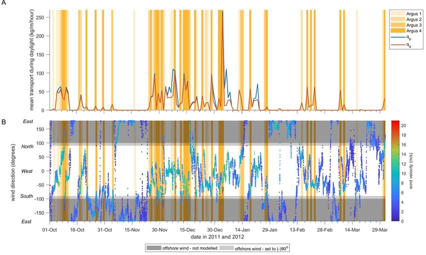
J. Mar. Sci. Eng. 2020, 8, 110                                                                         2 of 22

to cover the beach. According to these studies, a short fetch, i.e., the distance over which the wind
blows over the beach, and a large surface moisture content form important limitations for aeolian sand
transport. For arctic beaches, ice and snow cover form limiting factors as well [22], while nourished
beaches may have reduced aeolian transport because of shell lag deposits [24].
      To improve the prediction of aeolian sand transport on narrow beaches, ref. [3] proposed a series
of spatially explicit equations that include fetch distances. In addition to the fetch itself, they considered
the maximum possible fetch and a critical fetch, which is the downwind distance needed for aeolian
sand transport to reach its (potential) maximum. When the critical fetch is longer than the maximum
fetch, the maximum transport rate cannot be reached, and transport will be limited. The modelling
framework does not predict a quantitative transport rate, but it is a conceptual model capable of
calculating the spatial distribution of a relative sand transport rate as a function of the critical fetch
distance, beach geometry, and wind angle. The model was tested with data from a 9-month field
campaign at Greenwich Dunes, Canada, by [25] and further extended to be able to calculate sand
transport for limited transport conditions. The model of [25] forms the basis of this research and
extracts a beach width and uniform moisture content for the beach from video imagery. The model
applies several filter steps to select events likely to have transport. All events where no transport to
the dunes is expected are ignored: the wind must be above the threshold of sand entrainment and
have an onshore component, the gravimetric moisture content of the beach must be below 10%, the
beach should not be fully inundated, and ice and snow should not cover more than half the beach.
Then the critical fetch distance is determined from the wind velocity and increased with moisture
content, making it more likely that it will exceed the maximum fetch (causing limited transport) when
the beach is moist. Limited transport events will have a smaller transport rate, depending on the ratio
between the critical and maximum fetch. It was found that for the studied period at Greenwich Dunes,
the total transport rate was almost 29 times larger than the measured transport amount when only
wind direction and entrainment threshold were used as a filter. This diminished to a factor 11.8 when
the filter for snow cover, >10% moisture content, and an inundated beach were used. Including the
effect of fetch diminished it further to a factor 8.2, and when the full model was used, this became to
6.2 times the measured transport amount. The improved predictions for transport show the feasibility
of the fetch-approach, but the strong dependence on video data makes this model hard to apply to
unmonitored coastal sites.
      In this paper, we extend [25]’s work with a new fetch-based model, called Aeolus, which uses
time series of seawater elevation to determine groundwater cross-shore variability depth, which in
turn determines a spatially and temporally varying surface moisture content. Furthermore, the Aeolus
model determines the width of the beach, which is needed for calculating fetch distances, from a given
bed profile, wind, water level, and wave data. Here, we aim to qualitatively test the Aeolus model
for long time scales (months) by comparing its results to visual signs of aeolian sand transport at the
narrow beach of Egmond aan Zee, the Netherlands, previously explored in [21,23]. The predicted
transport will be compared with visual signs of aeolian transport, as determined from video monitoring.
In particular, we are interested to see if the model can provide a better match between predicted and
visually observed transport than a wind-alone model. The methodology is introduced in Section
2, including a description of the Aeolus model, field site, video monitoring data, model set-up and
synthetic runs. Section 3 describes our results. The discussion and conclusion can be found in Sections
4 and 5, respectively. A quantitative test of the model is left for future work.

2. Methodology

2.1. Model Description
     The Aeolus model consists of three modules. The first module is a groundwater model that
uses the non-linear Boussinesq equation for finite-amplitude water table fluctuations (e.g., [26]) with
a spatially constant aquifer thickness D. The Boussinesq equations follows from the substitution of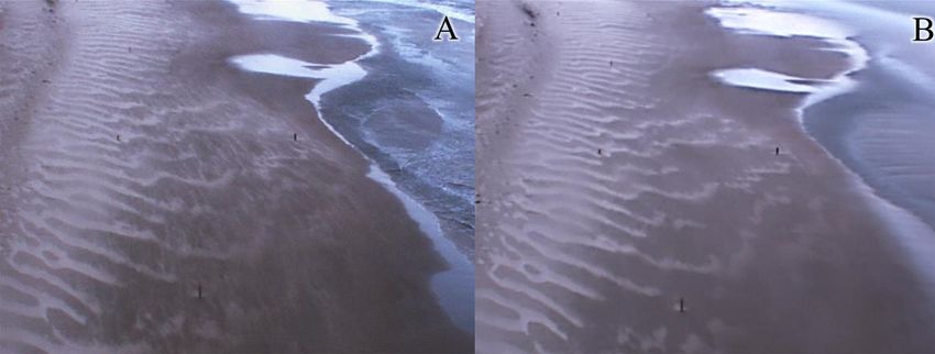
J. Mar. Sci. Eng. 2020, 8, 110                                                                            3 of 22

Darcy’s Law into the continuity equation [27]. Here, the Boussinesq equation is extended to include
infiltration by wave run-up, as proposed by [28,29]. The groundwater model assumes that the sand is
homogeneous and isotropic, and that groundwater flow is essentially horizontal, which is common for
sandy beaches [26]. The cross-shore (x) and temporal (t) evolution of the water table height η (m) with
respect to Mean Sea Level (MSL) is then

                                 ∂η ( x, t)   K ∂                     ∂η ( x, t)   U
                                            =       {[ D + η ( x, t)]            }+ l                        (1)
                                    ∂t        ne ∂x                      ∂x        ne

where K is the hydraulic conductivity of the beach (m/s), ne is the effective porosity (-), and Ul is the
run-up infiltration flow rate (m/s). Ul can be written as [28,30]
                                             (
                                                 Cl K f ( x ), if xc f ≤ x ≤ xru
                                      Ul =                                                                   (2)
                                                 0,            otherwise

where Cl is an infiltration coefficient (-) and f ( x ) is a function of x (-). xc f is the location where the
depth of the water table equals the thickness of the capillary fringe, and xru is the maximum run-up
location. Following [30], we let f ( x ) increase linearly from 0 at xc f to 1 at xru . The typical thickness for
the capillary fringe on a sandy beach is 0.1 to 0.2 m [31]. The parametrization by [32] was adopted to
compute xru . Refs. [30,33] mention the importance of wave run-up for accurately predicting η ( x, t)
above the high-tide level, especially when waves are energetic.
     Equation (1) was solved numerically, as described by [30], with a centered finite difference method
in space and a fourth-order Runge–Kutta integration technique in time. The seaward boundary
condition is a moving shoreline at location xsh (t) with elevation ηsh (t)

                                           ηsh ( xsh , t) = ζ 0 (t) + ξ sh (t)                               (3)

     It consists of the offshore water level ζ 0 (t) and the wave set-up ξ sh (t), estimated with offshore
wave data and the parametrization of [32]. The imposed landward boundary is ∂η/∂x = 0. The beach
profile must be monotonically increasing to apply Equation (1), meaning that intertidal sandbars and
troughs cannot be present. This part of the model needs a spin up time of approximately a month to
dampen and stabilize the strong fluctuations in the groundwater.
     The second part of the model determines the surface soil moisture of the beach. It is assumed
that the moisture profile above the water table is in hydrostatic equilibrium, meaning that the rising
and falling of the water table with time do not change the profile shape. The surface moisture thus
responds immediately to changes in the groundwater level. These assumptions are discussed in,
for example, Refs. [30,34], who argued that these assumptions are realistic unless the beach sand is
rather fine (≈150 µm). By adopting the water retention curve by [35], the gravimetric surface moisture
content ws can be related to the groundwater depth h as

                                                             wsat − wres
                                         ws = wres +                                                         (4)
                                                         [1 + (α|h|)n ]1−1/n

where wsat is the saturated water content (-), wres is the residual water content (-), and n is a measure
of the pore-size distribution (-). α (m−1 ) is related to the inverse of the air entry suction and affects the
thickness of the capillary fringe.
     The third module is based on the conceptual aeolian fetch model of [3], as extended by [25].
Ref. [3] proposed a parametrization of the increase in the aeolian transport rate q with downwind
fetch distance F, with q the product of the potential transport rate q p and a trigonometric function.
According to [36], the following function fits best with observations from agricultural fields

                                                                      π F
                                       q( F ) = min q p , q p × sin                                          (5)
                                                                      2 Fc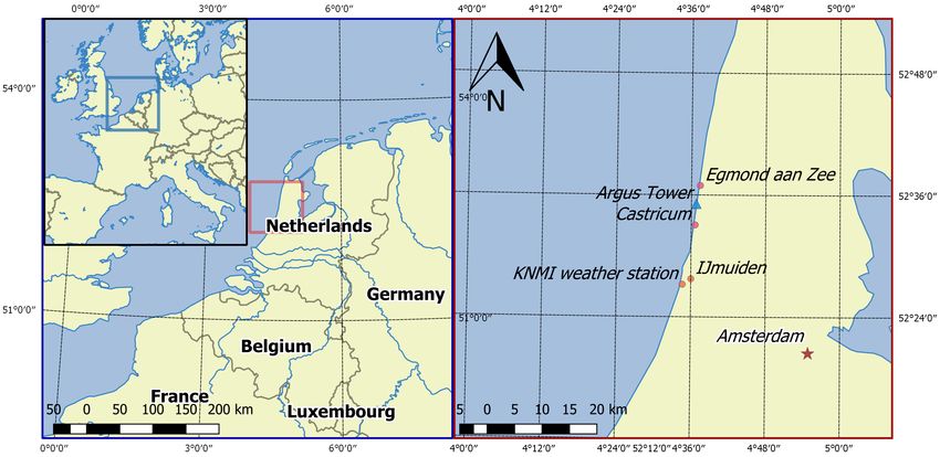
J. Mar. Sci. Eng. 2020, 8, 110                                                                             4 of 22

      In [36], Fc depends positively on wind speed U as Fc = 4.38 U − 8.23, and the computed value of
Fc is then modified based on ws . In [36], ws and the Fc modification are spatially constant. If ws is less
than 4%, Fc remains unchanged. If ws is between 4% and 6%, Fc increases with a factor 1.5, and if ws is
between 6 and 10%, Fc is 1.75 times as large compared to the dry-sand Fc . No transport is calculated if
ws is above 10%. In the Aeolus model, ws varies in the cross-shore direction, which implies that Fc is
spatially varying too. Therefore, Equation (5) was adapted into a spatially forward-stepping equation
                                 (      h                                     i
                                                                        F (i )
                                     min q p , q(i1 − 1) + q p × sin π2 F (i) ) ,    if ws (i ) ≤ ws,max
                      q (i ) =                                           c                                    (6)
                                     0,                                              otherwise

where i are spatial indices. When the most seaward gridpoint has a value less than the threshold value
ws,max set by the user, the computation of q starts. The remaining values for ws ( x ) are rounded to
multiples of 0.5% (now referred to as ws0 ). The fetch is the downwind distance over which the surface
moisture is constant, starting one spatial gridpoint upwind of the most upwind gridpoint of a group
of gridpoints with equal ws0 . This is indicated in Equation (5) with the i1 − 1 index. i thus refers to all
locations with constant ws0 . This approach causes F to reset to 0 with every change in ws0 . To avoid F
resetting for even tiny changes in ws , ws was rounded to multiples of 0.5%.
     The critical fetch in Aeolus is computed at each grid point as

                                                Fc (i ) = p(ws0 ) ∗ [4.38U − 8.23]                            (7)

     Based on the work of [5], p = 1 for ws0 ≤ 4% and a 0.125 increase in p per 1% increase in moisture.
q in Equation (6) is computed up and including the transition from beach to dune, which occurs at
elevation zup , a user-specified value. We refer to q at zup as the actual aeolian transport rate q a .
     The potential transport rate q p (kg m−1 s−1 ) is here computed following [2,37] as
                                                                                           !3
                                                                                  α U
                                 q p = 0.1 × [−0.47 + 4.97Dmm ] × 10         −4   pHsu                        (8)
                                                                                   gDcm

where U is the time-averaged (over 10 to 60 min) wind velocity measured at a height of 2 to 10 m. As in
[1], the grain size has to be specified in mm for Dmm and cm for Dcm and g = 981 cm/s2 . The parameter
α Hsu relates U to the shear velocity U∗ in cm/s can be determined with

                                                                   100κ
                                                       α Hsu =                                              (9)
                                                                 log zz0

where κ = 0.41 is Von Karman’s constant, z is the height above the bed where the wind velocity
is measured, and z0 is the roughness length. Based on extensive measurements, Ref. [1] proposed
α Hsu = 4.

2.2. Observations

2.2.1. Field Site
     The study site is located south of Egmond aan Zee, the Netherlands (Figure 1). The straight
coastline has an orientation of 7◦ east of north and consists of medium-fine sand with a median grain
size of about 240 µm. The beach is exposed to waves from the southwest to the north [38]. The Dutch
coast has a significant offshore wave period and height of 5 s and 1.2 m, respectively, which do not
show strong alongshore differences. During storms, the significant offshore wave height can increase
to over 5 m. Especially storms from the northwest are responsible for surges more than 1 m. As a result,
the intertidal beach can be flooded for several days [39]. The mean wind speed is 5.8 m/s, based on
wind data from 1981 to 2010 measured at de Kooy, 40 km north of the field site [40]. During storms, U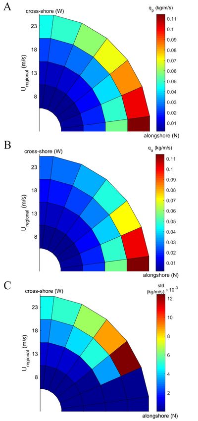
J. Mar. Sci. Eng. 2020, 8, 110                                                                     5 of 22

can attain values up to 30 m/s. The dominant wind direction at the site is south-southwest (210◦ –230◦
with respect to north).
     The semi-diurnal tide ranges from 1.4 m (neap tide) to 1.8 m (spring tide) and affects the width
of the beach, which usually varies between 30 and 100 m. The intertidal beach usually has one or
two slipface bars [41–43]. The high foredune (20 to 25 m) has a steep seaward front (40◦ –50◦ ) due
to occasional erosion events [44]. Large parts of the dune are covered in European marram grass
(Ammophila arenaria), especially at heights exceeding 10 to 15 m above beach level. During prolonged
periods of time without surges, embryo dunes can develop at the base of the foredune [45].

                                 Figure 1. Map of the field site and weather station.

2.2.2. Video Monitoring
     The beach south of Egmond aan Zee was monitored with an Argus video system [46] between
April 1998 and October 2015. Argus is an optical remote sensing system pioneered by Holman and
Sallenger [47] for sampling the nearshore environment. An Argus system consists of a suite of cameras
at the top of a high structure to gain an unhindered view of the beach. A timing module is installed to
ensure a synchronized collection of the images [48]. The Argus system at Egmond aan Zee consisted of
five RGB-color cameras, which were mounted on a 45-m high tower on the upper beach. The cameras
provided an 180◦ view, from south-southwest to north-northeast with a resolution of 640 × 480 pixels
from 1998 to February 2004, 1024 × 768 pixels from 2004 to August 2005 and 1392 × 1040 pixels until
2015. Every 30 min, each camera produced three different oblique images: a snapshot, a time-exposure
(timex) and a variance image. Only the first two types of images are used in this research. The timex
images were created by images taken with a frequency of 2 Hz over a 10-min period. This procedure
blurs out all movement in the 10-min time frame, such as individual waves breaking on the subtidal
bars and aeolian streamers on the beach. The movement of streamers is thus best noticeable when
a snapshot and timex of the same hour are compared: an active streamer can be seen on a snapshot
image, but not on a timex image (Figure 2). This makes them stand out from immobile, small, irregular
patches of dry sand that look like streamers on a snapshot image. Both snapshot and timex image
can be used to determine the movement of aeolian bedforms called sand strips (Figure 2), but as sand
strips move relatively slowly (a few meters per hour [21]), subsequent hourly images must be studied
to see their movement. The footprint dimensions of individual pixels (the projection of a square image
pixel on the ground) give the theoretical accuracy of the images, which is close to rectangular (with the
alongshore side being larger). For the post-2005 data, the cross-shore footprint dimension is less than
0.2 m, while the alongshore size increases from 0.2 m at 100 m from the tower alongshore to ≈1.5 m at
400 m.
     For each day in October 2011 to March 2012, the Argus image that showed the strongest signs of
aeolian sand transport was selected. The aeolian transport visible on the image was then classified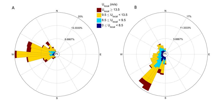
J. Mar. Sci. Eng. 2020, 8, 110 6 of 22
according to Figure 3. A second classification used the strongest 10-min-averaged wind velocity of
each day (Table 1), for which only daylight hours were used. The number of daylight hours is 11 h for
October and March, 9 h for November and February, and 8 h for December and January. These hours
were determined by observing the amount of light in Argus imagery.
Figure 2. An example of (A) a snapshot image and (B) a timex image. Streamers are visible on the
snapshot image (especially between sand strips), as a timex image blurs them out and shows the dark,
moist sand instead. Sand strips, on the other hand, move so slowly that they appear almost the same in
both images. The regional hourly mean wind velocity Uregional was 8 m/s and the wind direction θ
was −97◦ . Figure taken from [23].
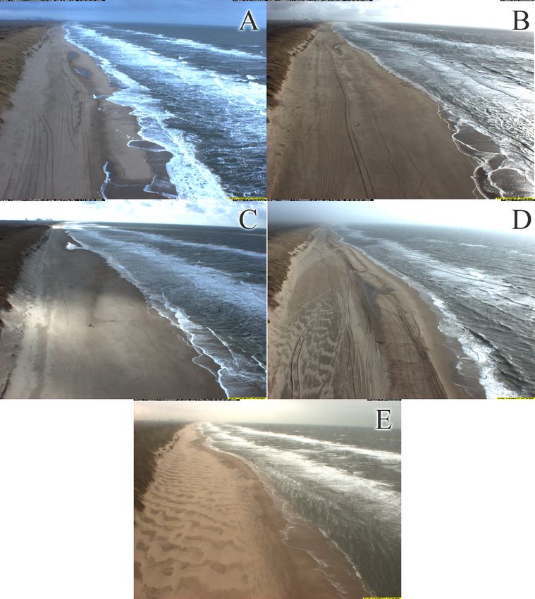
Figure 3. Snapshot images classified according to their visual signs of aeolian activity. (A) Class
0 shows no signs of transport; (B) class 1 shows very small signs of transport, like single moving
patches of sand or a handful of streamers; (C) class 2 has more of these sand patches, but they have not
formed rows of sand strips; (D) class 3 does have rows of sand strips, but the area they cover is patchy;
and (E) class 4 features sand strips that cover most of the beach, often in combination with strong
streamer activity. The date of the image and wind conditions were: (A) 08-02-2006, U = 7 m/s, θ = 23◦ ;
(B) 05-03-2006, U = 8 m/s, θ = 23◦ ; (C) 02-03-2006, U = 9 m/s, θ = −17◦ ; (D) 25-03-2006, U = 10 m/s,
θ = −47◦ ; (E) 10-11-2005, U = 12 m/s, θ = −57◦ . Taken from [23].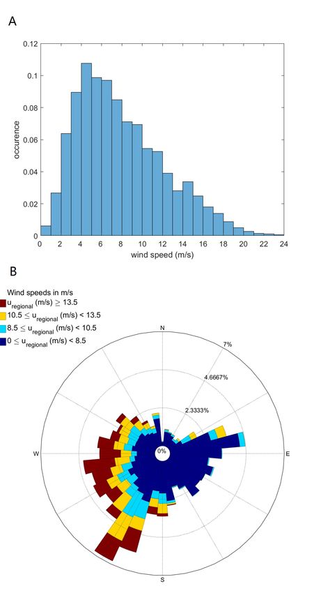
J. Mar. Sci. Eng. 2020, 8, 110                                                                             7 of 22

      Please note that the time intervals with the largest visual transport intensity is not necessarily
the same as the moment with the largest wind speed. Additionally, wind directions (θ) are reported
relative to shore normal in this paper, where θ = 0◦ is cross-shore and θ = 90◦ (−90◦ ) alongshore from
the north (south). The wind data were measured by the Royal Netherlands Meteorological Institute
(KNMI) in IJmuiden, roughly 15 km south of the field site (Figure 1).

      Table 1. Wind classes. The classification is based on the strongest hourly mean wind velocity measured
      regionally during daylight hours.

                                      Wind Class     Wind Velocity (m/s)
                                            1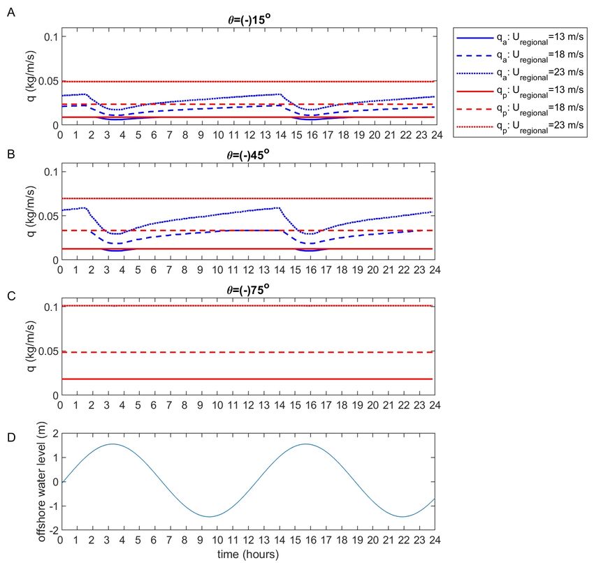
J. Mar. Sci. Eng. 2020, 8, 110                                                                       8 of 22

                     Table 2. Used settings for the Aeolus model to represent the Egmond beach.

                                           Spatial and temporal settings
               Start (dd-mm-yyyy)                                                  01-10-2011
               End (dd-mm-yyyy)                                                    31-03-2012
               Model output time step ∆t                                           10 min
               Spatial grid size ∆x                                                0.5 m
                                                Groundwater settings
               Calculation time step ∆t gw                                         2s
               Grid size                                                           0.5 m
               Aquifer depth D                                                     11 m
               Hydraulic conductivity K                                            4.63 × 10⁻⁴ m/s
               Effective porosity ne                                               0.3
               Infiltration coefficient Cl                                         0.5
               Minimum water table depth in run-up infiltration                    0.2 m
                                           Settings Van Genuchten curve
               Saturated water content wsat                                        20.51 %
               Residual water content wres                                         2.92 %
               α                                                                   5.59 m−1
               n                                                                   3.69
                                              Aeolian transport settings
               α Hsu                                                               4
               Grain size D50                                                      240 × 10−6 m
               Maximum surface moisture content ws,max                             10%
               Dunefoot elevation zup                                              2.5 m
               Minimum regional wind speed at which transport is possible Umin     8 m/s

                                         Figure 4. Smoothed Jarkus profile.

     The fetch model of Aeolus can only be run for aeolian transport towards the foredune, meaning
that any aeolian transport in the alongshore or offshore directions are set to zero. Sand transport with
offshore winds is rare at Egmond aan Zee, and when it happens, only small visual amounts of aeolian
transport are visible [23]. (Nearly) alongshore winds with a slight offshore direction, however, are
responsible for the strongest visual signs of aeolian transport [23,52]. Therefore, alongshore winds
between (-)90◦ and (-)100◦ (with 0◦ being cross-shore) were set to (-)90◦ to include these alongshore
winds in the calculations. This filter was not applied to the Argus imagery, as we were interested in the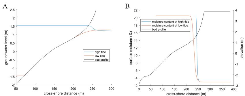
J. Mar. Sci. Eng. 2020, 8, 110                                                                       9 of 22

occurrence of sand transport under offshore winds and, therefore, when the wind direction is limiting
the model. The cosine effect [3,36,53] is not included, as the focus of this study is on the timing of
days with aeolian transport, not the amount of sand that will be deposited at the dune foot. The dune
foot elevation zup was set to 2.5 m, which is based on the beach profile at Egmond aan Zee (Figure 4).
This is a little larger than the 2% exceedance value of the wave run-up maxima at the field site, which
is 2.23 m in the studied period.

      Figure 5. The correction factor needed when computing the local from regional wind velocities as
      a direction of regional wind direction. 0◦ is cross-shore (onshore).

2.4. Synthetic Runs
      Several synthetic simulations were run to illustrate the output of the model and to aid in the
interpretation of the Egmond simulations. We focus here on moisture and, in particular, aeolian
transport rates, as output from the groundwater model have already been discussed extensively
in [30,34]. The imposed conditions were a semi-diurnal tide of 12 h and 25 min with an amplitude
of 1.5 m and a wave period and height of 5 s and 1.2 m, respectively. The regional wind direction θ
varied from 0◦ to ±90◦ (with 0◦ being onshore) with a 15◦ step size and the regional wind speed was
varied from 8 to 23 m/s with intervals of 5 m/s for each direction. To mimic the Egmond situation,
the regional wind speed was transformed to the local wind. All other variables and parameters were
set to fit the Egmond site (see Section 2.3). Each simulation was run for 30 days to account for the
model’s spin up time. The results below focus on the 30th day.
      Figure 6 shows the output of the surface moisture model. The upper part of the intertidal zone
(between 220 and 240 m) slowly dries during low tide, and inundates quickly with rising tide. Please
note that most of the intertidal beach remains too wet to sustain aeolian transport (ws >10%). Figure 7
shows nine examples of the synthetic runs, displaying the actual transport rate q a at zup = 2.5 m (at
x ≈ 260 m in Figure 6), the potential transport rate q p based on [1], and the imposed offshore tide.
Obviously, q p does not depend on time, but because of the imposed wind speed correction it does
depend on θ. In contrast, q a can vary with time, as it does, for example, when θ = 15◦ and Uregional = 18
or 23 m/s (Figure 7A). The largest values for q a were not reached at low tide when the beach is at its
widest, but approximately 2 h before high tide, when the surface moisture at the upper intertidal zone
is smallest, hence providing the largest surface of dry sand (Figure 6). The groundwater level keeps on
falling until the beach is inundated by the tide. The groundwater level and surface moisture content at
high tide (time = 3:21 h in Figure 7) and low tide (time = 9:36 h in Figure 7) are shown in Figure 8A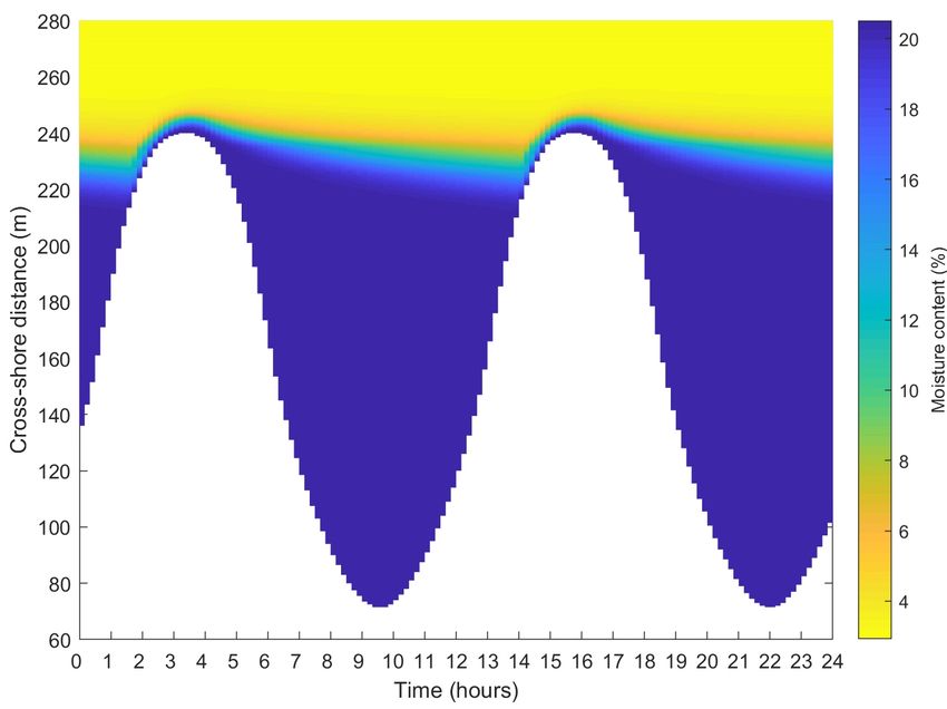
J. Mar. Sci. Eng. 2020, 8, 110                                                                            10 of 22

and B, respectively. The groundwater level is close to the bed for most parts of the intertidal beach
during the tidal cycle and the surface moisture always keeps its maximum value, wsat . Only around
x= 240 m, the surface moisture drops below 10% to allow aeolian transport during certain parts of the
tide. Qualitatively, this is consistent with suggestions in [30,54] that the contribution of the intertidal
zone as a sand source for aeolian transport is limited.
       In general, q a is less than q p for θ = 15◦ , except for the smallest wind velocity Uregional = 13 m/s.
Then, q a is smaller than q p during high tide only (Figure 7A). The larger the wind velocity, the larger
the difference between q a and q p . Similar results can also be seen for θ = 45◦ (Figure 7B), but not when
θ = 75◦ (Figure 7C). Now, q a = q p in all simulations. This (lack of) difference between q a and q p is
further illustrated in Figure 9. Both q a and q p , averaged for a single tide, increase when the wind
becomes more alongshore, and the wind speed increases. For q p (Figure 9A), the difference with θ
is caused by the wind speed correction while for q a , θ also affects the maximum fetch. When the
angle of the wind is almost alongshore, the critical fetch length Fc is reached and exceeded even at
high tide, which causes q a and q p to be the same. Little to no potential and actual transport can be
expected for small wind velocities no matter the direction. Figure 9C shows the standard deviation in
q a . A zero standard deviation implies q a does not vary with the tide. This happens when the wind
is (almost) alongshore. The critical fetch is then reached during the entire tidal cycle. With oblique
winds, the maximum fetch length varies greatly, allowing the critical fetch to be (almost) reached only
during low tide. This results in the largest standard deviations. With cross-shore winds, the maximum
fetch length still varies, but it will do so less than for oblique winds, and, consequently, the standard
deviation reduces again.

      Figure 6. Surface moisture model output for a 12.5 h tide with an amplitude of 1.5 m, a wave height of
      1.2 m, a wave period of 5 s, and using the parameters and bed profile for Egmond aan Zee. The figure
      depicts the model output for day 30 of the studied time period. The cross-shore distance runs from the
      sea (bottom of the figure) to the dunes (top of figure).
J. Mar. Sci. Eng. 2020, 8, 110 11 of 22
Figure 7. Aeolian transport rate q a as calculated by Aeolus and the potential transport rate q p based
on wind velocity alone at x ≈ 260 m (zup = 2.5 m) for (A) θ = 15◦ , (B) θ = 45◦ , and (C) θ = 75◦ . This
transport does not take the cosine effect into account. (D) shows the tide for reference.
Figure 8. (A) Groundwater level during high and low tide and (B) surface moisture during high and
low tide modelled by Aeolus.J. Mar. Sci. Eng. 2020, 8, 110 12 of 22
Figure 9. (A) Mean potential aeolian transport rate q p for various wind velocities and directions,
(B) mean actual aeolian transport rate q a , and (C) the standard deviation in q a , calculated for a single
tide and various wind velocities and directions. There are 4 values for the regional wind velocity, which
increase from inner to outer ring, and 7 different wind directions.
3. Results
The most common regional wind speed during the studied time period from October 2011 to
March 2012 was around 5 m/s (Figure 10A), while the average regional wind speed was 6.6 m/s.J. Mar. Sci. Eng. 2020, 8, 110 13 of 22
The largest wind speed encountered was 24 m/s. The dominant wind direction was south-west,
followed by nearly westerly winds (Figure 10B). Westerly winds also showed a relatively large
percentage of strong winds (>13.5 m/s).
Table 3 displays the number of days with transport sorted according to their largest
10-min-averaged wind velocity measured during daylight hours and their strongest visual signs
of transport. A few days (November 10, 17, and 21) could not be studied as fog obscured the beach
during the entire day. Most of the 183 days show either no (class 0, 126 days) or substantial visual
signs (class 4, 28 days) of aeolian transport. According to [23], strong winds but no or limited transport
indicate supply-limited conditions at the beach. How large the wind speed has to be for limited
transport depends on the strength of the visual aeolian transport; a transport day with no visual sign
of transport is considered limited when the wind speed is above the threshold of transport (≈8 m/s
for Egmond aan Zee). The wind speed must be larger when stronger visual signs are present. That
means that all days of visual transport class 0 in Table 3, many of visual transport class 1, and some of
visual transport class 2 and 3 are probably limited.
Table 3. Days sorted according to their wind class (Table 1) and visual transport class (Figure 3), with
the total number of days for each class and the corresponding percentage.
Visual Transport Class
Wind Class 0 1 2 3 4 Total Percentage
1 84 1 1 1 0 87 47.5%
2 20 4 4 1 10 39 21.3%
3 15 5 1 3 5 29 15.8%
4 7 4 1 3 13 28 15.3%
Total 126 14 7 8 28 183
Percentage 68.8% 7.7% 3.8% 4.4% 15.3%
Figure 11A shows the hourly average predicted potential and actual transport during daylight
hours, together with the strongest visual classification of Argus imagery of the corresponding day.
The corresponding wind direction and velocity is shown in Figure 11B. Visual signs of aeolian transport
were especially common in the end of November and in December 2011, during which the wind was
relatively strong. March 2012, in contrast, had weak winds and contained only a few Argus images with
visual transport. Offshore winds usually do not create aeolian bedform, which was the case for most
days in November. This corresponds qualitatively with the model predictions, which are largest during
the second half of November and December. The day with the largest average predicted potential
and predicted actual transport is 3 January 2012, reaching 265.4 and 251.2 kg/m/h, respectively.
The intensity of the visual signs of aeolian transport on the Argus images generally corresponds
with the amount of predicted actual transport, with a stronger visual class generally having a larger
predicted actual transport. There are, however, several days (e.g., October 5, 6, 7, and 12, 2011), for
which q a was predicted to be relatively large (≈50 kg/m/h, which was almost the same as q a on those
days), but Argus showed minimal signs of aeolian activity (class 1). The other way around, with
small q a (≈10 kg/m/h), but strong visual signs of transport (class 4), happened occasionally too (e.g.,
October 21, 26, and 30).
On 30 of the total 183 days the model predictions and Argus observations did not agree in the
sense that Argus showed no transport but q a was non-zero. These mismatches tend to occur on
days with little transport, as on 27 days the potential transport was less than 10% of the maximum
predicted potential transport. This may imply that small transport rates are not well visible, and are
thus incorrectly classified as transport class 0. On 5 days, visual signs of transport were present, but
the model predicted zero q a . These mismatches will be examined further in the Discussion section of
this paper.J. Mar. Sci. Eng. 2020, 8, 110 14 of 22
Figure 10. (A) Histogram of the wind speed and (B) a windrose showing the direction and speed of
the wind at the KNMI weather station in IJmuiden from October 2011 to March 2012. The coastline has
an approximate north-south orientation.J. Mar. Sci. Eng. 2020, 8, 110 15 of 22
Figure 11. (A) Time series of predicted hourly average potential and actual transport (daylight hours only) and the strongest observed visual transport for each day.
(B) the corresponding wind direction and velocity. Aeolus cannot model offshore wind. Winds that were offshore, but nearly alongshore (with θ between (-)90◦ and
(-)100◦ ) were set to θ = (-)90◦ .J. Mar. Sci. Eng. 2020, 8, 110 16 of 22
Figure 11A illustrates that q a was often predicted to be regularly smaller than q p , in other words,
that transport at the dune line is limited. Table 4 provides the average ratio of q a and q p for each
visual class (using daily sums of daylight hours only for all cases with non-zero q p ). Several days, but
especially in visual transport class 0 (97 out of 126), result in q p = q a = 0. This is caused by offshore
winds filtered out by Aeolus, except for wind class 1; here, the non-zero values are almost all caused by
a wind speed smaller than the threshold of motion (40 of these days showed a combination of a small
wind speed and an offshore wind). Two days with offshore wind form an exception. Even though
the wind speed on these days surpassed the threshold of motion, it did not cause any visual signs of
aeolian transport (visual transport class 0).
The q a to q p ratios are (close to) 1 for most wind and visual transport classes. The smallest ratios
for q a /q p can be found in strong wind classes (class 3 and 4) with little visual transport (class 0 and
1). Some classes contain only a few days, which makes it hard to draw conclusions, but the general
trend of small q a /q p for strong wind classes (class 3 and 4) in combination with small visual transport
classes (class 0 and 1) corresponds to the expectation of limited transports for these conditions. Also,
q a /q p ≈ 1 otherwise is consistent with expectations. Strong winds with little visible transport seem
to be fetch limited, or were classified as having no visual transport because the aeolian transport is
too small to be visible on the imagery. It was found in [23] that weak winds could still cause a large
amount of aeolian bedforms, but probably only when there is sufficient time to develop them.
Table 4. Mean q a /q p for the days from Table 3. When there is no number, there either are no days that
fall within this wind and visual transport class or q a and q p are zero. The numbers between parentheses
show the number of days where q a and q p are non-zero and the total number of days in that class.
Visual Transport Class
Wind Class 0 1 2 3 4
1.00 - - - -
1
(2 out of 84) (0 out of 1) (0 out of 1) (0 out of 1) (0 out of 0)
0.94 0.99 0.98 - 1.00
2
(11 out of 20) (3 out of 4) (4 out of 4) (0 out of 1) (10 out of 10)
0.77 0.91 0.91 0.98 1.00
3
(10 out of 15) (5 out of 5) (1 out of 1) (3 out of 3) (5 out of 5)
0.46 0.76 0.88 0.98 0.98
4
(6 out of 7) (4 out of 4) (1 out of 1) (3 out of 3) (13 out of 13)
The ratio of q a /q p depends on the wind speed and direction. The wind rose in Figure 12A is based
on wind data with q a /q p < 0.8 and in Figure 12B with q a /q p ≥ 0.8. When q a /q pJ. Mar. Sci. Eng. 2020, 8, 110 17 of 22
Figure 12. (A) Wind rose consisting of transport days when q a /q pJ. Mar. Sci. Eng. 2020, 8, 110 18 of 22
January 2012 on the other hand, showed a medium strong visual sign of transport (class 3), even though
the wind velocity did not exceed the threshold of motion. The period of visual aeolian transport lasted
no more than an hour. The wind causing it might have been too local to be registered by the weather
station in IJmuiden, and therefore resulted in a q a of zero. Also, wind gusts above the threshold may
have caused some transport, but gustiness is not included in Aeolus. The images of 26 January 2012
showed strong signs of transport (class 4). The wind direction was larger than 100◦ for most of the day,
meaning its transport rate was set to zero by Aeolus. On this day, the days when the wind direction
was less than 100◦ , the wind velocity was below the threshold of motion. This case shows that the
threshold of 100◦ might not have been large enough to include all days that cause alongshore aeolian
transport. Offshore winds that have a more cross-shore direction usually do not cause visible signs
of aeolian transport at the Egmond study site, which makes Aeolus work reasonably well for this
site. This might not be the case for other beaches, where studying and modelling aeolian transport
events by offshore events, as was done by [55,56], is far more essential. Overall, most Argus-Aeolus
mismatches are thus induced by poor classification of Argus imagery, where the visual signs of aeolian
transport are too small to be observed properly. For a few cases, precipitation and frost could be the
cause of a mismatch. Exceeding the wind direction threshold was the cause of a mismatch for one day.
Finally, we note that the days with strong signs of aeolian transport did not always coincide
with large predicted transport rates (Figure 11). Underdeveloped or no sand strips (class 0, 1, and 2),
however, do seem to be more common when q a differs strongly from q p , which can be seen for October
5 and 6, December 5 to 7, January 4 to 7, and January 20 to 22. The development of sand strips might
be hindered by a moist surface or a short fetch during these days, meaning that well-developed signs
of aeolian transport are more likely to appear on days with unhindered sand transport, not necessarily
on days with large potential transport rates.
4.2. Relevance of Days with Limited Transport
Although, as indicated in Table 4, the ratio of q a to q p is often large, the days when q a is well
below q p do have a large influence on the cumulative transport in the study period. This is further
illustrated with Figure 13. The total q p and q a from October 2011 to March 2012 (including night hours)
is 6.6 × 10⁴ kg/m and 5.2 × 10⁴ kg/m, respectively. The amount of sand that reaches the dune foot
(implementing the cosine effect) is 3.7 × 10⁴ kg/m and 2.7 × 10⁴ kg/m for q p and q a , respectively.
This amount is larger than observed (see also [13]), as the dune volume at this site increases with
2.3 × 10⁴ kg/m/year during accretion periods [57]. An interesting future step is to calculate aeolian
transport rates in supply-limited conditions, like the AeoLis model developed by [58].
Both q a and q p follow a comparable cumulative trend, but their difference does not increase
gradually with time. Instead, only a few individual days seem to invoke sudden, substantial differences
(e.g., 5 to 9 December 2011 and 3 January 2012). It is interesting to note that only parts of these days
had limited transport. During the days in December, the wind was strong (>11 m/s) and fluctuated
in direction. When it was (close to) cross-shore, it caused limited transport. January 3 started with
very strong winds of ≈20 m/s. Since these winds were shore-oblique, the fetch length was close to
the critical fetch length, causing q a /q p to fluctuate between 1.00 (low tide) and 0.80 (high tide). Only
when the wind changed to a more cross-shore direction at the end of the day, q a /q p dropped to 0.45.
This further stresses that the limitation in only a few days with large potential transport may have
a profound effect on long-term aeolian transport. Future work is needed to test the generality of this
finding, including in-depth analyses of these complex events and the possibility of increasing the
temporal resolution of visual transport classifications from daily to hourly.J. Mar. Sci. Eng. 2020, 8, 110 19 of 22
Figure 13. Cumulative sum of Q a and Q p , and their difference.
5. Conclusions
The Aeolus model was developed to make better predictions of aeolian sand transport rates on
narrow beaches by including wind- and moisture-induced fetch effects. To test if the model predicts
the timing and transport-limited nature of aeolian transport events correctly, its results were compared
to Argus images collected during a six-month winter period at Egmond aan Zee (the Netherlands).
The medium to strong transport events predicted by Aeolus usually coincided with strong visual
signs of aeolian transport in the images. Consistent with visual signs of limited transport, Aeolus
sometimes predicted the actual transport to be smaller than the potential transport. Strong differences
are more common for strong and onshore winds. Furthermore, it was observed that strong visual signs
of aeolian transport overlapped with either equal actual and potential transport (i.e., no limitation), or
when the actual transport was relatively large. Mismatched days usually had no visual sign of aeolian
transport on the corresponding Argus images and only small transport rates predicted by Aeolus. It
is possible that these aeolian transports are too small to be seen on Argus, or that a limiting factor
not taken into account by Aeolus, like rain or snow, was enough to end this small amount of aeolian
transport. This semi-quantitative research shows that overall, the Aeolus model predicts the timing of
sand transport well for a long, multiple-month time period.
Author Contributions: conceptualization, P.H. and G.R.; methodology, P.H., G.R.; software, P.H., G.R., Z.v.A.;
validation, P.H., G.R. and J.D.; formal analysis, P.H.; investigation, P.H., Z.v.A.; resources, G.R.; data curation,
P.H.; writing—original draft preparation, P.H.; writing—review and editing, G.R. and J.D.; visualization, P.H.;
supervision, G.R. and J.D.; project administration, G.R.; funding acquisition, G.R. All authors have read and
agreed to the published version of the manuscript.
Funding: This study was funded by the Dutch Technology Foundation STW (Vici project 13709), which is part
of the Netherlands Organisation for Scientific Research (NWO), and which is partly funded by the Ministry of
Economic Affairs.
Acknowledgments: We wish to thank Bas van Dam, the late Irv Elshoff, John Stanley and Rob Holman for
Argus support. We also want to thank Irene Delgado-Fernandez and Bernard Bauer for their extensive feedback.
Conflicts of Interest: The authors declare no conflict of interest. The funders had no role in the design of the
study; in the collection, analyses, or interpretation of data; in the writing of the manuscript, or in the decision to
publish the results.J. Mar. Sci. Eng. 2020, 8, 110 20 of 22
References
1. Hsu, S.A. Computing Eolian Sand Transport from Routine Weather Data. Coast. Eng. 1974, 1619–1626.
[CrossRef]
2. Davidson-Arnott, R.G.D.; Law, M.N. Measurement and prediction of long-term sediment supply to coastal
foredunes. J. Coast. Res. 1996, 12, 654–663.
3. Bauer, B.O.; Davidson-Arnott, R.G.D. A general framework for modeling sediment supply to coastal dunes
including wind angle, beach geometry, and fetch effects. Geomorphology 2002, 49, 89–108. [CrossRef]
4. Sherman, D.J.; Houser, C.; Baas, A.C.W. Electronic Measurement Techniques for Field Experiments in Process
Geomorphology; Elsevier Ltd.: New York, NY, USA, 2013; Volume 14, pp. 195–221. [CrossRef]
5. Delgado-Fernandez, I.; Davidson-Arnott, R.G.D. Meso-scale aeolian sediment input to coastal dunes:
The nature of aeolian transport events. Geomorphology 2011, 126, 217–232. [CrossRef]
6. Edwards, B.L.; Namikas, S.L. Small-scale variability in surface moisture on a fine-grained beach: implications
for modeling aeolian transport. Earth Surf. Process. Landf. 2009, 34, 1333–1338. [CrossRef]
7. Wiggs, G.F.S.; Atherton, R.J.; Baird, A.J. Thresholds of aeolian sand transport: establishing suitable values.
Sedimentology 2004, 51, 95–108. [CrossRef]
8. Nield, J.M.; King, J.; Wiggs, G.F.S.; Leyland, J.; Bryant, R.G.; Chiverrell, R.C.; Darby, S.E.; Eckardt, F.D.;
Thomas, D.S.G.; Vircavs, L.H.; et al. Estimating aerodynamic roughness over complex surface terrain.
J. Geophys. Res. Atmos. 2013, 118, 12948–12961. [CrossRef]
9. Nield, J.M.; King, J.; Jacobs, B. Detecting surface moisture in aeolian environments using terrestrial laser
scanning. Aeolian Res. 2014, 12, 9–17. [CrossRef]
10. Svasek, J.N.; Terwindt, J.H.J. Measurements of sand transport by wind on a natural beach. Sedimentology
1974, 21, 311–322. [CrossRef]
11. Jackson, N.L.; Nordstrom, K.F. Aeolian transport of sediment on a beach during and after rainfall, Wildwood,
NJ, USA. Geomorphology 1998, 22, 151–157. [CrossRef]
12. Sherman, D.J.; Jackson, D.W.; Namikas, S.L.; Wang, J. Wind-blown sand on beaches: An evaluation of
models. Geomorphology 1998, 22, 113–133. [CrossRef]
13. de Winter, W.; Donker, J.; Sterk, G.; Van Beem, J.; Ruessink, G. Regional versus local wind speed and
direction at a narrow beach with a high and steep foredune. PLoS ONE 2020, 15. [CrossRef] [PubMed]
14. Bauer, B.O.; Davidson-Arnott, R.G.; Nordstrom, K.F.; Ollerhead, J.; Jackson, N.L. Indeterminacy in aeolian
sediment transport across beaches. J. Coast. Res. 1996, 12, 641–653.
15. Bauer, B.O.; Davidson-Arnott, R.G.D.; Hesp, P.A.; Namikas, S.L.; Ollerhead, J.; Walker, I.J. Aeolian sediment
transport on a beach: Surface moisture, wind fetch, and mean transport. Geomorphology 2009, 105, 106–116.
[CrossRef]
16. Baas, A.C.W.; Sherman, D. Formation and behavior of aeolian streamers. J. Geophys. Res. Earth Surf. 2005, 110.
[CrossRef]
17. Sherman, D.J.; Li, B. Predicting aeolian sand transport rates: A reevaluation of models. Aeolian Res. 2012,
3, 371–378. [CrossRef]
18. Montreuil, A.L.; Chen, M.; Brand, E.; Strypsteen, G.; Rauwoens, P.; Vandenbulcke, A.; De Wulf, A.; Dan, S.;
Verwaest, T. Dynamics of Surface Moisture Content on a Macro-tidal Beach. J. Coast. Res. 2018, 85, 206–210.
[CrossRef]
19. Nield, J.M.; Wiggs, G.F.S.; Squirrell, R.S. Aeolian sand strip mobility and protodune development on a drying
beach: examining surface moisture and surface roughness patterns measured by terrestrial laser scanning.
Earth Surf. Process. Landf. 2011, 36, 513–522. [CrossRef]
20. Nield, J.M. Surface moisture-induced feedback in aeolian environments. Geology 2011, 39, 915–918.
[CrossRef]
21. Hage, P.M.; Ruessink, B.G.; Donker, J.J.A. Determining sand strip characteristics using Argus video
monitoring. Aeolian Res. 2018, 33, 1–11. [CrossRef]
22. Delgado-Fernandez, I.; Davidson-Arnott, R.G.D.; Ollerhead, J. Application of a Remote Sensing Technique
to the Study of Coastal Dunes. J. Coast. Res. 2009, 255, 1160–1167. [CrossRef]
23. Hage, P.M.; Ruessink, B.G.; Donker, J.J.A. Using Argus video monitoring to determine limiting factors of
aeolian sand transport on a narrow beach. J. Mar. Sci. Eng. 2018, 6, 138. [CrossRef]J. Mar. Sci. Eng. 2020, 8, 110 21 of 22
24. Van der Wal, D. Effects of fetch and surface texture on aeolian sand transport on two nourished beaches.
J. Arid Environ. 1998, 39, 533–547. [CrossRef]
25. Delgado-Fernandez, I. Meso-scale modelling of aeolian sediment input to coastal dunes. Geomorphology
2011, 130, 230–243. [CrossRef]
26. Raubenheimer, B.; Guza, R.; Elgar, S. Tidal water table fluctuations in a sandy ocean beach. Water Resour.
Res. 1999, 35, 2313–2320. [CrossRef]
27. Nielsen, P. Tidal dynamics of the water table in beaches. Water Resour. Res. 1990, 26, 2127–2134. [CrossRef]
28. Nielsen, P.; Davis, G.; Winterbourne, J.; Elias, G. Wave setup and the watertable in sandy beaches. Tech. Rep.
Tech. Memo-Randum 1998, 88, 1.
29. Kang, H.Y.; Nielsen, P.; Hanslow, D.J. Watertable overheight due to wave runup on a sandy beach. Coast.
Eng. 1994, 2115–2124.
30. Brakenhoff, L.B.; Smit, Y.; Donker, J.J.; Ruessink, G. Tide-induced variability in beach surface moisture:
Observations and modelling. Earth Surf. Process. Landf. 2019, 44, 317–330. [CrossRef]
31. Turner, I.L.; Nielsen, P. Rapid water table fluctuations within the beach face: Implications for swash zone
sediment mobility? Coast. Eng. 1997, 32, 45–59. [CrossRef]
32. Stockdon, H.F.; Holman, R.A.; Howd, P.A.; Sallenger Jr, A.H. Empirical parameterization of setup, swash,
and runup. Coast. Eng. 2006, 53, 573–588. [CrossRef]
33. Huizer, S.; Karaoulis, M.; Oude Essink, G.; Bierkens, M. Monitoring and simulation of salinity changes in
response to tide and storm surges in a sandy coastal aquifer system. Water Resour. Res. 2017, 53, 6487–6509.
[CrossRef]
34. Smit, Y.; Donker, J.; Ruessink, B. Spatiotemporal surface moisture variations on a barred beach and their
relationship with groundwater fluctuations. Hydrology 2019, 6, 8. [CrossRef]
35. Van Genuchten, M.T. A closed-form equation for predicting the hydraulic conductivity of unsaturated soils
1. Soil Sci. Soc. Am. J. 1980, 44, 892–898. [CrossRef]
36. Delgado-Fernandez, I. A review of the application of the fetch effect to modelling sand supply to coastal
foredunes. Aeolian Res. 2010, 2, 61–70. [CrossRef]
37. Hsu, S.A. Wind stress criteria in eolian sand transport. J. Geophys. Res. 1971, 76, 8684–8686. [CrossRef]
38. Wijnberg, K.M.; Terwindt, J.H.J. Extracting decadal morphological behaviour from high-resolution, long-term
bathymetric surveys along the Holland coast using eigenfunction analysis. Mar. Geol. 1995, 126, 301–330.
[CrossRef]
39. Quartel, S.; Ruessink, B.G.; Kroon, A. Daily to seasonal cross-shore behaviour of quasi-persistent intertidal
beach morphology. Earth Surf. Process. Landf. 2007, 32, 1293–1307. [CrossRef]
40. Sluijter, R.; Leenaers, H.; Camarasa, M. De Bosatlas van het klimaat; Noordhoff uitgevers Groningen:
Groningen, The Netherlands, 2011. Available online: www.klimaatatlas.nl (accessed on 11 February 2020).
41. Masselink, G.; Kroon, A.; Davidson-Arnott, R.G.D. Morphodynamics of intertidal bars in wave-dominated
coastal settings—A review. Geomorphology 2006, 73, 33–49. [CrossRef]
42. Aagaard, T.; Kroon, A.; Andersen, S.; Sørensen, R.M.; Quartel, S.; Vinther, N. Intertidal beach change during
storm conditions; Egmond, The Netherlands. Mar. Geol. 2005, 218, 65–80. [CrossRef]
43. Quartel, S.; Grasmeijer, B.T. Dynamiek van het strand bij Noordwijk aan Zee en Egmond aan Zee en het
effect van suppleties. In Rijksinstituut voor Kust en Zee (RIKZ); Opdracht RKZ-1667; Universiteit van Utrecht:
Utrecht, The Netherlands, 2007.
44. de Winter, R.C.; Gongriep, F.; Ruessink, B.G. Observations and modeling of alongshore variability in dune
erosion at Egmond aan Zee, the Netherlands. Coast. Eng. 2015, 99, 167–175. [CrossRef]
45. Ruessink, B.; Schwarz, C.; Price, T.; Donker, J. A Multi-Year Data Set of Beach-Foredune Topography and
Environmental Forcing Conditions at Egmond aan Zee, The Netherlands. Data 2019, 4, 73. [CrossRef]
46. van Enckevort, I.M.J.; Ruessink, B.G. Effect of hydrodynamics and bathymetry on video estimates of
nearshore sandbar position. J. Geophys. Res. Oceans 2001, 106, 16969–16979. [CrossRef]
47. Holman, R.A.; Sallenger, A.H. High-energy nearshore processes. Eos Trans. Am. Geophys. Union 1986,
67, 1369. [CrossRef]
48. Holman, R.A.; Stanley, J. The history and technical capabilities of Argus. Coast. Eng. 2007, 54, 477–491.
[CrossRef]
49. Tuijnman, Y. Soil Moisture Dynamics and the Effects on Initiation of Aeolian Sand Transport; Utrecht University:
Utrecht, The Netherlands, 2019.J. Mar. Sci. Eng. 2020, 8, 110 22 of 22
50. Smit, Y. Surface Moisture Dynamics on a Narrow Coastal Beach. Ph.D. Thesis, Utrecht University, Utrecht,
The Netherlands, 2019.
51. Ruessink, G.; Schwarz, C.; Hage, P.; Smit, Y.; de Winter, W.; Donker, J. Predicting Potential Aeolian Sand
Supply to a High and Steep Foredune. In Proceedings of the AGU Fall Meeting Abstracts, Washington, DC,
USA, 10–14 December 2018.
52. Bauer, B.O.; Davidson-Arnott, R.G.; Walker, I.J.; Hesp, P.A.; Ollerhead, J. Wind direction and complex
sediment transport response across a beach–dune system. Earth Surf. Process. Landf. 2012, 37, 1661–1677.
[CrossRef]
53. Davidson-Arnott, R.; Dawson, J. Moisture and fetch effects on rates of aeolian sediment transport, Skallingen,
Denmark. In Proceedings of the Canadian Coastal Conference, Canadian Coastal Science and Engineering
Association, Ottawa, ON, Canada, 5–9 November 2001; pp. 309–321.
54. Schmutz, P.; Briggs, T.; Tereszkiewicz, P. The utility of an omni-directional photoelectronic sensor device to
measure meso-scale variability in aeolian sediment transport activity. Aeolian Res. 2019, 36, 61–67. [CrossRef]
55. Jackson, N.L.; Nordstrom, K.F. Aeolian sediment transport and landforms in managed coastal systems:
A review. Aeolian Res. 2011, 3, 181–196. [CrossRef]
56. Delgado-Fernandez, I.; Jackson, D.W.; Cooper, J.A.G.; Baas, A.C.; Beyers, J.M.; Lynch, K. Field
characterization of three-dimensional lee-side airflow patterns under offshore winds at a beach-dune
system. J. Geophys. Res. Earth Surf. 2013, 118, 706–721. [CrossRef]
57. Donker, J.; van Maarseveen, M.; Ruessink, G. Spatio-temporal variations in foredune dynamics determined
with mobile laser scanning. J. Mar. Sci. Eng. 2018, 6, 126. [CrossRef]
58. Hoonhout, B.M.; Vries, S.D. A process-based model for aeolian sediment transport and spatiotemporal
varying sediment availability. J. Geophys. Res. Earth Surf. 2016, 121, 1555–1575. [CrossRef]
© 2020 by the authors. Licensee MDPI, Basel, Switzerland. This article is an open access
article distributed under the terms and conditions of the Creative Commons Attribution
(CC BY) license (http://creativecommons.org/licenses/by/4.0/).You can also read