The Impact of Tides on the Bay of Biscay Dynamics - MDPI
←
→
Page content transcription
If your browser does not render page correctly, please read the page content below
Journal of
           Marine Science
           and Engineering

Article
The Impact of Tides on the Bay of Biscay Dynamics
John Karagiorgos ∗ , Vassilios Vervatis                   and Sarantis Sofianos
 National and Kapodistrian University of Athens, Department of Physics, 15772 Athens, Greece;
 vervatis@oc.phys.uoa.gr (V.V.); sofianos@oc.phys.uoa.gr (S.S.)
 * Correspondence: jkaragiorgos@oc.phys.uoa.gr

 Received: 17 July 2020; Accepted: 13 August 2020; Published: 17 August 2020

 Abstract: The impact of tides on the Bay of Biscay dynamics is investigated by means of an ocean
 model twin-experiment, consisted of two simulations with and without tidal forcing. The study is
 based on a high-resolution (1/36◦ ) regional configuration of NEMO (Nucleus for European Modelling
 of the Ocean) performing one-year simulations. The results highlight the imprint of tides on the
 thermohaline properties and circulation patterns in three distinct dynamical areas in the model
 domain: the abyssal plain, the Armorican shelf and the English Channel. When tides are activated,
 the bottom stress is increased in the shelf areas by about two orders of magnitude with respect to
 the open ocean, subsequently enhancing vertical mixing and weakening stratification in the bottom
 boundary layer. The most prominent feature reproduced only when tides are modelled, is the Ushant
 front near the entrance of the English Channel. Tides appear also to constrain the freshwater transport
 of rivers from the continental shelf to the open ocean. The spectral analysis revealed that the tidal
 forcing contributes to the SSH variance at high frequencies near the semidiurnal band and to the
 open ocean mesoscale and small-scale features in the presence of summer stratification pattern.

 Keywords: ocean modelling; tides; vertical mixing; energy spectra; NEMO; bay of biscay

1. Introduction
     Tides are a key physical process for understanding and modelling the 3D ocean circulation,
especially in shelf seas and near the coast. Tidal forcing contributes substantially to the simulation
of mixing and transport through different mechanisms such as nonlinear interactions between tidal
currents and the general circulation, mixing induced by internal tides and energy dissipation through
bottom friction (see, e.g., in [1–4]). The authors of [5] suggest that the inclusion of tides in global ocean
models allows a better representation of processes at regional scales. Moreover, barotropic tide models
are often used to calibrate observations derived from altimetry missions (see, e.g., in [6]). There are
two common approaches to include tides in the ocean model simulations: either with direct simulation
or parameterisation. In this work, we examine the prospects of the first method through the study of
the impact of tides on a regional ocean model from a dynamical point of view.
     The Bay of Biscay, located in the northeast Atlantic Ocean, is a semi-enclosed sea supporting a
large number of human activities that include fisheries, shellfish farming, shipping and oil transport.
Beyond its social-economic interest, the Bay of Biscay is characterised by a variety of physical
and hydrographical properties [7] constrained by a complex topography, i.e., varying width of the
continental shelf from south to north, a steep continental slope, canyons and the abyssal plain with
typical depths of ~4500 m. The most intense circulation patterns in this region are explained by coastal
density-driven flows controlled by tidal dynamics over the continental shelf [8,9], a slope current along
the northern Spanish coast and over the Armorican shelf break with seasonal reversals [10–12] and
several long-lived anticyclonic eddies in the open-ocean [13,14]. Moreover, the cross-shelf exchanges
documented in the area regulate the interaction of the continental shelf and the deep ocean [15–18].

J. Mar. Sci. Eng. 2020, 8, 617; doi:10.3390/jmse8080617                           www.mdpi.com/journal/jmse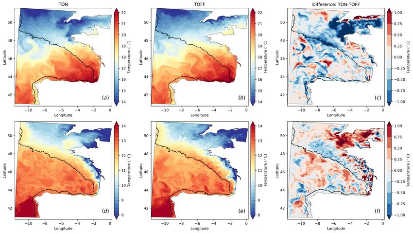
J. Mar. Sci. Eng. 2020, 8, 617                                                                       2 of 17

     Tides in the Bay of Biscay are highly energetic [8,9] and the region is notably known for being one
of the major generation spots of internal tidal waves [19]. The interaction of barotropic tidal currents
with the steep slopes at the shelf break generates internal tides of large amplitude during periods
of intense seasonal thermocline, propagating from the shelf break towards the shelf and the abyssal
plain [20–23]. The known sites for the generation of internal tides in the Bay of Biscay is the Armorican
shelf break around 47◦ N [23] and along the West-Iberian continental slope [22]. A large fraction of
these waves dissipate locally in shallow areas [24] through wave breaking, enhancing mixing along the
continental shelf break. The interaction of tidal currents with the bottom topography is also responsible
for the formation of seasonal thermal fronts in the Bay of Biscay, such as the Ushant front [12,25,26].
The Ushant front is the most significant tidal front in the study area shaping the circulation in the
English Channel and associated with ecosystem dynamics (see, e.g., in [27]).
     There have been several studies investigating the location and the dynamics of frontal activity in
the Northwest European shelf [28–32]. The authors of [33] are the first to study the physical mechanisms
related to the generation of tidal fronts in coastal regions, proposing a criterion for the occurrence of
fronts. They showed that tidal fronts are observed in areas of intense tidal mixing (i.e., weakening of
the stratification) where there is also buoyancy gain in the ocean led by thermal fluxes (i.e., enhancing
the stratification). The balanced interaction between these two mechanisms leads to a temperature
contrast between the well-mixed waters on one side of the front and stratified waters on the other side
of the front. According to the work in [33], the location of a tidal front can be identified by calculating
a parameter known as the Simpson–Hunter (SH) parameter, taking under account the depth and the
averaged velocity of the water column.
     In this study, we investigate the impact of barotropic tides (and their baroclinic effect) on the
Bay of Biscay dynamics, using a high-resolution (1/36◦ ) regional configuration. We compare the
results from a twin-experiment based on two ocean model simulations, with and without tidal forcing.
The main objective is to quantitatively assess the dynamical changes brought by tides in a wide range
of spatio-temporal scales, both in the open ocean and on the shelves. The paper is organised as follows.
Section 2 presents the numerical model set-up, the experimental design and methodology. Section 3
provides a quantitative assessment of the thermohaline properties and the dynamical aspects of tides
in the Bay of Biscay using also spectral analysis. Finally, Section 4 gives the concluding remarks of the
present study.

2. Ocean Model Simulations and Methodology

2.1. Numerical Model and Set-Up
      A regional configuration of the Nucleus for European Modelling of the Ocean (NEMO; http:
//www.nemo-ocean.eu/ [34]) has been used with a 1/36◦ horizontal resolution and 50 vertical levels.
The model domain is a subgrid of the Iberian–Biscay–Irish (IBI) model [35,36], inherited from earlier
studies [37,38], and extends between 11◦ to 0.26◦ W in longitude and 41◦ to 51.5◦ N in latitude
including the Bay of Biscay and the western part of the English Channel (Figure 1). The bathymetry
was constructed using GEBCO 08 data-set (30 arc-second resolution; http://www.gebco.net) and
regional bathymetries [35]. For more technical details and for the validation of this configuration the
reader is referred to [35].
      The meteorological fields were provided from the European Centre for Medium-Range Weather
Forecasts (ECMWF) atmospheric operational model analysis, with a 0.25◦ horizontal resolution and
3 h time interval. The fields include the 10-m wind velocity, 2 m air temperature and relative humidity,
downwelling long and shortwave radiation and atmospheric pressure. The wind stress and the
surface fluxes were estimated using the bulk formula of [39]. The initial state and the open boundary
conditions were provided by the daily outputs of the Mercator Ocean operational system named
PSY2v3 (1/12◦ ). The river runoffs are based on daily discharges (https://wwz.ifremer.fr/) at three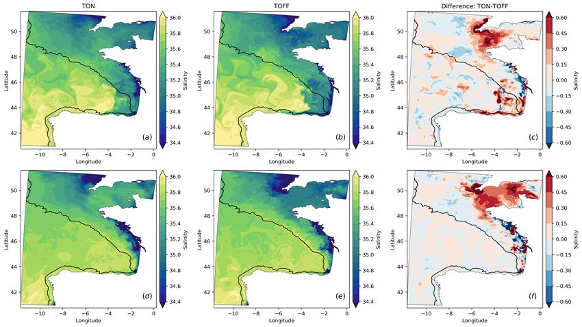
J. Mar. Sci. Eng. 2020, 8, 617                                                                                  3 of 17

sites of major rivers, namely, the Loire (2.19◦ W, 47.27◦ N), Gironde (0.73◦ E, 45.26◦ N) and Adour
(1.52◦ E, 43.53◦ N).
      Tides are included in the model by calculating the astronomical tidal potential and the tidal
harmonic forcing in the open boundaries. The tidal forcing in the boundaries was provided by the
TPXO 7.1 global tide model [40] as the sum of 11 constituents: (a) diurnal constituents (K1, O1, P1 and
Q1), (b) semi-diurnal constituents (M2, S2, N2 and K2), (c) long-period-tides (Mf and Mm) and (d)
a nonlinear constituent M4 (compound tides). An important ocean model parameterisation related to
tides, especially in the shallow macrotidal shelf regions of the present configuration, was the calculation
of a quadratic bottom drag coefficient using a logarithmic formulation, considering also the bottom
roughness (important over the shelves) [35].
      The bottom drag is estimated online, calculating the water column dynamical variations in the
lowest bottom cell thickness (i.e., the partial cells). The latter parameterisation allowed for a more
realistic representation of the bottom stress, as opposed to other non-dynamical parametrizations
(e.g., constant values or formulation of the bottom drag), taking under account the interplay between
vertical shear, stretching of the water column and mixing in the model. The vertical mixing is based on
the Generic Length Scale (GLS) turbulent closure scheme. We used the k-epsilon parameterisation and
the Canuto type A stability functions [41,42]. The scheme is based on the prognostic transport equations
of the turbulent kinetic energy and the generic length scale, for the production of turbulence by shear
and buoyancy, using a Neumann boundary condition. Away from the boundaries, the background
viscosity and diffusivity were limited using a Galperin coefficient at 0.267 for the dissipation rate and a
minimum background of turbulent kinetic energy at 10−6 m2 s−2 . These model parameterisations have
also been used in [35] in the IBI domain. Finally, an inverse barometer signal was also added to the sea
level at open boundaries.

      Figure 1. Bathymetry of the Bay of Biscay configuration in meters. The red box and dots depict the area and
      stations calculating model diagnostics. The black lines represent the 100, 200 and 1000 m isobaths.

2.2. Design of the Twin-Experiment
     We carried out a twin-experiment consisting of two simulations: (a) one with a tidal forcing
(hereafter, tides-on: TON) and (b) one without tidal forcing (hereafter, tides-off: TOFF) for a period
of one year from July 2011 to June 2012. The tidal motion in the TON experiment is induced in the
model by both tidal potential and open boundary conditions. Other than that, the two simulations
have identical atmospheric forcing, initial conditions, and the slow components of open boundary
conditions of the thermohaline properties and velocities. We note that both simulations have identical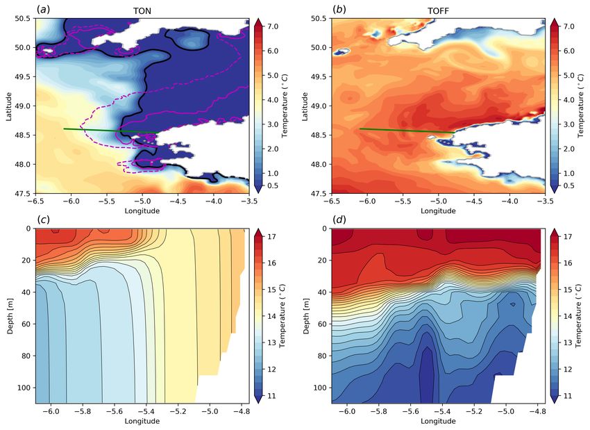
J. Mar. Sci. Eng. 2020, 8, 617                                                                         4 of 17

model set-up for the bottom drag coefficient and the vertical mixing scheme, with the only difference
being the vertical velocity shear and the stretching of the water column, when tides are activated in
the model. The prognostic model variables are stored at hourly intervals for both simulations to assess
the high-frequency motions due to tides.

2.3. Methodology
       As a first step, we analysed model outputs from the TON and TOFF simulations, comparing the
model prognostic variables and other diagnostics, such as the relative vorticity, the flow divergence
and the Brunt-Väisälä frequency, between the two simulations. In a second step, we performed spectral
analysis both in frequency and wavenumber domain to quantitatively assess the impact of tides on the
spectral characteristics of the Bay of Biscay dynamics.
       A quantification of the water column structure can be provided by the Brunt-Väisälä frequency
N 2 , computed by the polynomial expression of [43] as follows,

                                                     g ∂ρ      ∂T      ∂S
                                   N 2 ( T, S) = −        ≈ gα    − gβ                                    (1)
                                                     ρ ∂z      ∂z      ∂z

where a is the thermal expansion coefficient; b is the haline contraction coefficient; g is the gravity field;
T and S are the potential temperature and salinity profiles, respectively; and z is the depth. For the
calculation of the Brunt-Väisälä, the relative vorticity ζ = (v x − uy ) and flow divergence σ = (u x + vy )
diagnostics, we used the CDFTTOOLS package (https://github.com/meom-group/CDFTOOLS).
     A Fast Fourier Transform analysis for the Sea Surface Height (SSH) variance was performed to
estimate the energy spectrum as a function of frequency. A Welch filter [44] and a temporal Hanning
window of approximately 2 days was applied to hourly segments, to remove noise and highlight the
dominant spectral peaks. The calculations were performed for the two simulations and over typical
locations shown in Figure 1, i.e., stations depicted with red dots in the abyssal plain, Armorican shelf
and the English Channel.
     The energy associated with motions of different spatial scales was quantified using a wavenumber
spectral analysis. We used the pyspec package (https://github.com/pyspec/pyspec) to estimate the
horizontal isotropic wavenumber spectrum [45] from the model hourly fields in a subdomain spanning
the abyssal plain 6.1◦ –10.1◦ W, 44.4◦ –47.2◦ N (Figure 1; red box). The selected subdomain includes
spatially homogeneous ocean circulation patterns constrained in the abyssal plain by the continental
slope. The spectral method incorporates a two-dimensional Discrete Fourier Transform, applying
also a spatial smoothing Hanning window of an order of 3 km and removing the spatial averages.
The spectrum was azimuthally averaged per wavenumber [45].
     As proposed in [33], we also calculated the tidal mixing parameter (referred as the Simpson–Hunter
parameter; hereafter SH) to identify the location of tidal fronts and intense tidal mixing:

                                            SH = log10 (h/U 3 )                                           (2)

where h is the water depth in meters and U is the depth-averaged tidal velocity in m/s. According to
the authors of [33], the fronts should be located in areas with a critical SH parameter value. These SH
values can be used to identify specific areas of intense tidal mixing. By definition, the SH parameter is
estimated when tides are included in the model (i.e., here the TON simulation). When SH values are
small, there is a homogenisation of the water column, in particular in regions dominated by strong tidal
currents [28]. For the Northwest European shelf, and specifically in the English Channel, the critical
SH values reported in the literature [29,30] are between 2.7 and 3.0. In the results section, the SH
parameter computed over the summer period is also compared to the temperature difference between
surface and bottom waters (i.e., ∆T = Tsur f ace − Tbottom ), to highlight areas of intense tidal mixing.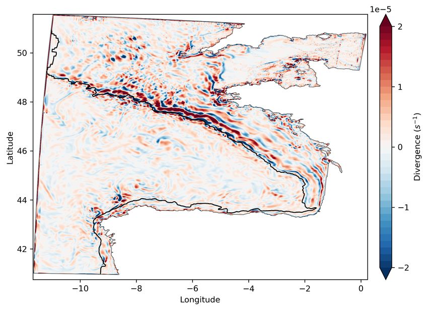
J. Mar. Sci. Eng. 2020, 8, 617                                                                         5 of 17

3. Results
     In this section, we investigate the impact of tidal forcing on the Bay of Biscay by comparing the
results of the two model simulations (TON and TOFF). We consider the differences in the thermohaline
properties, the circulation patterns and the evolution of the stratification in different areas of the
domain. Finally, we perform spectral analysis of the SSH evolution, in order to identify the impact of
tides on the energy distribution at different time and spatial scales.
     As an illustration of the tidal forcing applied in the TON simulation (and excluded from the TOFF
simulation), we present in Figure 2 the amplitude and phase of M2 and M4 tidal constituents. M2 is
the major tidal constituent in the Northeast Atlantic Ocean with amplitudes exceeding 3 m in the
domain (Figure 2a). M4 is a principal quarter-diurnal compound tide generated from the interaction
of M2 with itself. The M4 amplitude is more significant over the continental shelf than the abyssal
plain, with maximum amplitudes localised in the Armorican shelf and the English Channel (Figure 2b).
The tidal map of M4 shows two amphidromic points (zero amplitude) located in the English Channel
as described by [46].

      Figure 2. Amplitude in meters (colour) and phase (black lines; amphidromic points: zero amplitude)
      of modelled (a) M2 and (b) M4 tidal constituent.

3.1. Distribution of Thermohaline Properties
       Figures 3–5 present the observational data OSTIA [47] and the modelled Sea Surface Temperature
(SST) and Salinity (SSS), respectively. The data and model results are illustrated for two representative
days at the end of summer (upper panels) and in mid-winter (lower panels). In Figures 4 and 5,
the left panels correspond to the TON simulation, the middle panels to the TOFF simulation and
the right panels to their difference “TON minus TOFF”. In summer, both simulations reproduce the
characteristic “warm pool” in the southeastern corner of the Bay of Biscay (Figure 4a,b), with SST
values exceeding 20 ◦ C verified also by the OSTIA-SST satellite observations (Figure 3a). During the
same period and over the Celtic and Armorican shelves, we observe the Ushant tidal front at the
entrance of the English Channel (48.2◦ N, 5.6◦ W) in the OSTIA-SST dataset and only in the realistic
TON simulation; we observe cold waters at about 15◦ C in the vicinity near the coasts and warmer
waters outside the front (Figures 3a and 4a). During winter, there is a marked spatial variability in
hydrography with warmer and generally saltier waters in the open ocean compared with the shelves
(i.e., by approximately 12–13 ◦ C and 35.6–35.8; Figures 3b, 4d and 5d). A thermal front observed in the
OSTIA-SST and in both simulations during winter, separates the coastal cold waters (i.e., values do not
exceed 10 ◦ C) of the Armorican shelf influenced by the river plumes, with the open ocean warm waters.
The same period, in the abyssal plain, we observe the presence of coherent eddies and filaments in both
simulations, leaving a clear imprint of the circulation pattern on the SST and SSS fields (Figures 4d,e
and 5d,e) in contrast with the smoothed OSTIA fields (Figure 3b). When we validate the model with
in situ observations at the Channel Lightship station (49.9◦ N 2.9◦ W; https://marine.copernicus.eu;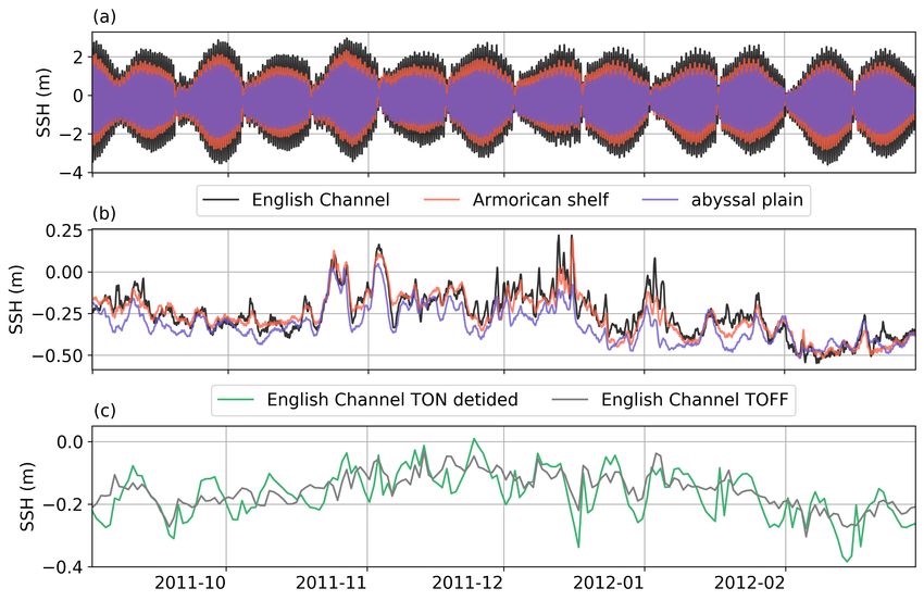
J. Mar. Sci. Eng. 2020, 8, 617                                                                            6 of 17

Figure S1), we find that the TON simulation has smaller Mean Absolute Error (MAE) at about 0.59 ◦ C
over the simulation period, as opposed to the TOFF experiment with MAE 0.85 ◦ C.

      Figure 3. Sea surface temperature (◦ C) from OSTIA L4 satellite observations on (a) 28 September 2011
      and (b) 24 February 2012.

       Differences in SST between TON and TOFF simulations suggest that the addition of tidal forcing
produces high spatial changes of SST locally exceeding 1 ◦ C (Figure 4c,f). The tidal forcing contribution
to the SST fields is different in the two periods. For example, during summer, the SST is colder when
tides are activated, while the opposite is true during the winter period (Figure 4c,f). In summer,
the SST is colder in TON compared with the TOFF simulation in the English Channel, the shelves
(near the continental shelf break at approximately 47◦ N) and in the Spanish continental slope at
approximately 43.5◦ N (Figure 4c). The largest temperature differences are locally observed in the
position of the Ushant front, which is formed only in the TON simulation (Figure 4a–c). The latter
result is of substantial importance as oceanic fronts play a key role in the circulation of shelf seas which
are regions of intense biological activity. Another finding is that the northern coast of the English
Channel has warmer SSTs than the rest of the Channel when tides are activated, which can affect the
ocean model’s skill to represent the SST compared to satellite observations (cf. [48]).
       Examining the differences in winter, the SST is warmer when tides are activated, notably in the
English Channel and in the largest part of the abyssal plain (Figure 4f). In the Armorican shelf, we
observe small-scale contrasting positive–negative SST fields for the difference “TON minus TOFF”
(i.e., differences up to 1 ◦ C), attributed on the frontal displacement of the river plumes. The latter
is also in agreement with the coastal SSS fields modulated by the river plumes (Figure 5f). In the
same area, along the continental slope at about 4◦ W to 9◦ W, the SST appears to be colder in the
simulation with tides than without tides. This SST cooling is less intense compared with values
observed during summer (Figure 4c). This cooling is most likely associated with internal tides breaking
in the continental slope and subsequently enhancing mixing in the shelves, bringing cold bottom
waters on the surface (cf. also [21]).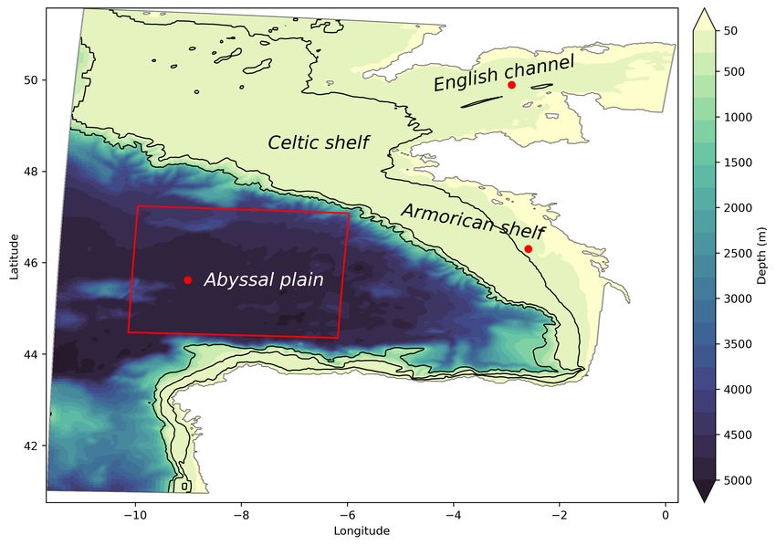
J. Mar. Sci. Eng. 2020, 8, 617                                                                          7 of 17

      Figure 4. Sea surface temperature (◦ C) on (a–c) 28 September 2011 and (d–f) 24 February 2012 for
      tides-on (TON) and tides-off (TOFF), and their difference “TON minus TOFF”, respectively. The black
      line indicates the 200-m isobath, which delimits the shelf break.

                                 Figure 5. Same as Figure 4 for the sea surface salinity.

     In Figure 5c,f, we present the differences in SSS between the two simulations and the two periods.
The greatest differences are observed in the English Channel (i.e., greater than 0.6), most notably in the
entrance of the Channel (near 48.5◦ N, 4◦ W). This is possibly explained by the fact that the Ushant
front acts as a barrier to the intrusion of low salinity waters (i.e., values < 35.2; cf. [49]), originated
from the Loire and Gironde rivers. We note that the SSS increases (in both periods) in the English
Channel when tides are activated, in contrast to SST which only increases in the TON simulation
and only during the winter. The rivers freshwater transport from the shelves to the open ocean is
constrained when tides are activated in the model simulation, probably due to changes in stratification
and mixing (discussed in Section 3.3). This pattern is observed during summer, when occurring high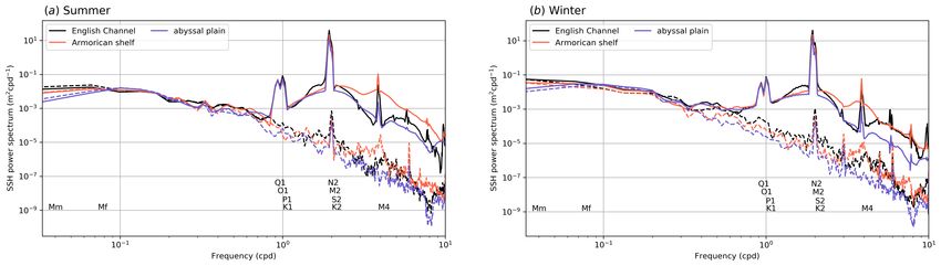
J. Mar. Sci. Eng. 2020, 8, 617                                                                              8 of 17

salinity differences (i.e., values up to 0.6) in the transition area of the Landes Plateau at approximately
44.5◦ N, 3.5◦ W (Figure 5c).
     Figure 6a,b shows the temperature difference between the surface and bottom waters during
summer for the TON and TOFF simulations. As shown in Figure 6a, the English Channel is an area
characterised by intense tidal mixing, illustrated by ∆T with values lower than 0.5 ◦ C. The location
of the Ushant front can be identified by the ∆T isotherm of 0.5 ◦ C (Figure 6a; black line) and the area
spanned by the 2.7 and 3.0 contours of the Simpson–Hunter parameter (Figure 6a; magenta lines).
In the simulation without tides, ∆T has greater values than the 0.5 ◦ C threshold (e.g., up to 7 ◦ C)
confirming the absence of fronts in the area (Figure 6b). Figure 6c presents the longitudinal cross
section of the water column temperature near the entrance of the English Channel. The cross section
was selected in the area where the ∆T isotherm of 0.5 ◦ C and the SH contours are collocated, denoting
the presence of the Ushant tidal front (Figure 6a). We observe a homogenisation of the water column
east of 5.4◦ W (Figure 6c). On the contrary, in the simulation without tides, we observe a well-formed
seasonal thermocline at approximately 40 m depth (Figure 6d).

      Figure 6. (a,b) Surface minus bottom temperature on 28 September 2011 for TON and TOFF in a zoom
      area near the entrance of the English Channel. (c,d) Vertical cross sections of temperature along green
      lines shown in subplots (a,b). The magenta lines in subplot (a) present the values of Simpson–Hunter
      parameter for the contours of 2.7 (solid) and 3.0 (dashed) respectively, and the solid black line the
      contour of ∆T = 0.5 ◦ C.

3.2. Relative Vorticity and Divergence
     In this section, we investigate the relative vorticity and surface divergence fields to assess the
dynamical impact of tides on the Bay of Biscay mesoscale activity. In Figure 7, we depict the relative
vorticity, with and without tides, for the same dates as in the SST and SSS fields. As expected, during
winter, we observe in both simulations more intense circulation patterns in the abyssal plain compared
with the summer circulation, attributed to coherent and more energetic eddies and vortices constrained
in the abyssal plain by the continental slope.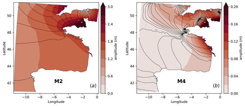
J. Mar. Sci. Eng. 2020, 8, 617 9 of 17
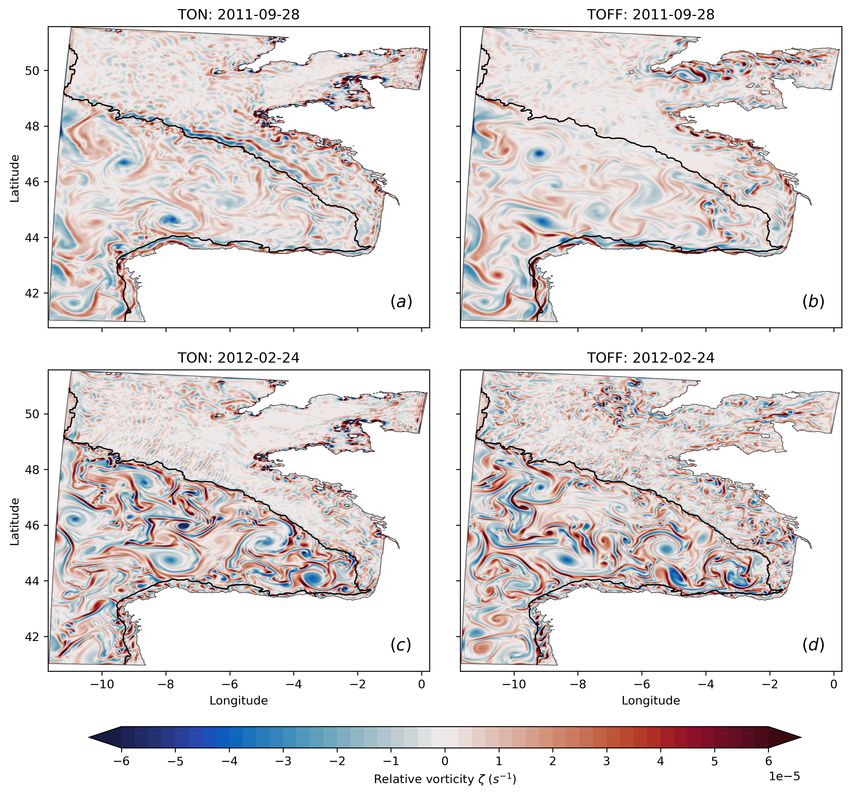
Figure 7. Surface relative vorticity (s−1 ) for (a,b) 28 September 2011 and (c,d) 24 February 2012. Panels
(a,c) correspond to the TON simulation and panels (b,d) to the TOFF simulation respectively.
Near the shelf break and only during summer in the TON simulation, there is a crest-through
signal of internal tides propagation in the Armorican and Celtic shelves at approximately
47◦ –48◦ N 5◦ –7◦ W (Figure 7a). During winter, when tides are activated, the relative vorticity fields
present small-scale structures, especially in the Armorican shelf near the coasts and the Loire and
Gironde river discharges (Figure 7c).
During summer, when tides are included in the simulation, there is a marked increase in relative
vorticity over the Armorican and Celtic shelves at approximately 47◦ –48◦ N and 4◦ –8◦ W, compared
with the TOFF simulation (Figure 7b). On the other hand, during the same period, the relative
vorticity is decreased in the northern part of the English Channel in the presence of tidal forcing
(Figure 7a,b). During winter, there are evidences of small-scale vortices over the Armorican shelf in
Figure 7d (TOFF simulation), confirmed also previously by the winter temperature and salinity fields
(cf. Figures 4e and 5e). In the same period over the abyssal plain, we observe an increase of mesoscale
activity southern to the shelf break in the TON simulation, i.e., 47◦ N, 7◦ W, near the generation area
of internal tides (Figure 7c,d). Overall, when tides are included, small-scale and mesoscale activity
weakens on the shelves during both periods and increases in the open-ocean, notably southern to the
shelf break and during summer when stratification is strong.
In this study, we depict also the summer divergence of the surface circulation for the TON
experiment, as a means to investigate the dynamics of internal tides in our model domain (Figure 8).
There are evidences of spatial patterns with positive/negative values of divergence flow, denoting
the vertical variations in the water column as a result of internal tides. We note that, in the TOFF
experiment, this divergence pattern is totally absent (i.e., lower values at about two orders of magnitude
compared with the TON simulation; not shown). In more detail, we observe high values of divergence
flow along the continental shelf slope, most notably at 47◦ –48◦ N, 4◦ –8◦ W and in agreement with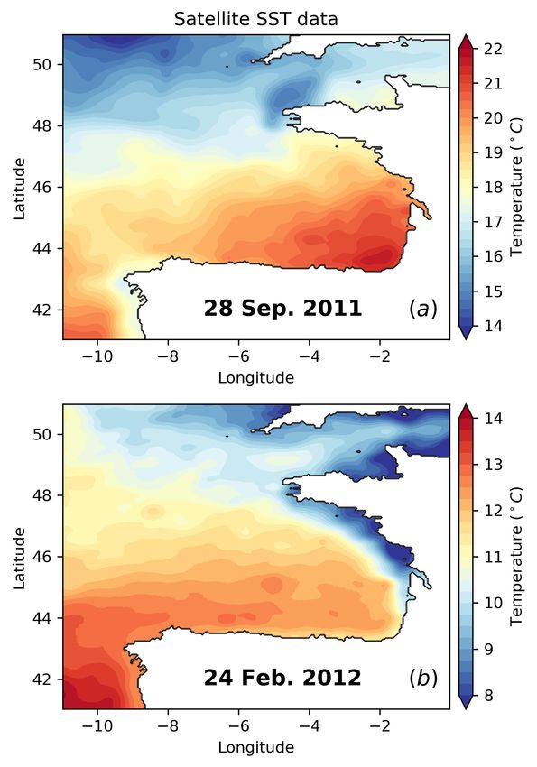
J. Mar. Sci. Eng. 2020, 8, 617                                                                             10 of 17

the literature, characterised as a hot spot area of internal tides generation, due to the interaction
of barotropic tides with the steep slope [20–23]. In addition, we observe a crest-through signal of
divergence flow (more apparent compared with vorticity) gradually reducing its signal as we move
away from the continental slope. The signal over the Armorican shelf dissipates near the coastal
regions and in the English Channel near the location of the Ushant front.

      Figure 8. Surface divergence of the horizontal flow (s−1 ) on 28 September 2011 for the TON simulation.
      The divergence for the TOFF experiment is two orders of magnitude smaller; not shown.

3.3. Vertical Stratification
      We calculate the Brunt-Väisälä frequency N 2 (Equation (1)), using the daily modelled profiles
of potential temperature and salinity at selected stations depicted in Figure 1, to quantify the impact
of tides on the vertical stratification. Figure 9 shows Hovmöller plots of the Brunt-Väisälä frequency
for the Armorican shelf and the English Channel stations, respectively. The impact of tides on the
vertical stratification of the abyssal plain is negligible (except locally near the continental shelf break)
and therefore, not shown here for the two simulations.

      Figure 9. Hovmöller plots of the Brunt-Väisälä frequency (s−2 ) calculated for (a,c) the TON and
      (b,d) TOFF daily model outputs. The upper panels correspond to the Armorican shelf station and the
      lower panels to the English Channel station.
J. Mar. Sci. Eng. 2020, 8, 617 11 of 17
During winter we observe near-zero values for the Brunt-Väisälä frequency in both simulations,
indicating strong mixing due to surface heat loss over the shelves and nearly homogenous conditions in
the water column structure (Figure 9; white areas between December and March). The most prominent
differences in the Brunt-Väisälä frequency between the two simulations are observed in summer and
during transition periods (i.e., spring/fall), when there is a strong stratification due to the thermocline
shoaling. The changes brought by tides in the water column are visible in the Armorican shelf at
depths below the seasonal thermocline and down to the seabed, and in the English Channel over the
whole water column.
The stratification in the Armorican shelf below the seasonal thermocline, i.e., from 20 to 50 m
depth, shows high variations and appears to be weaker when tidal forcing is activated, compared with
the smoother vertical profiles and the stronger stratification when tides are excluded (Figure 9a,b).
An interesting remark, is that when tides are activated in the model, the vertical stratification in
the English Channel vanishes (almost) completely during the transition periods and in summer, as
opposed to the simulation without tides (cf. lack of dark blue colour in Figure 9c against Figure 9d).
The mechanism controlling the changes in the vertical stratification over the shelves is associated
with the bottom Ekman flow pattern. In the presence of tides, the bottom stress (and its coefficient)
is increased, leading to an increase in the vertical velocity shear and mixing in the shelf areas of the
English Channel dominated by strong tidal currents. In order to quantify this impact, we calculated the
bottom stress when tides were activated and we found an increase by about one order of magnitude
larger in the Armorican shelf (i.e., values up to 0.1 N/m2 ) and two orders of magnitude larger in the
English Channel (i.e., values up to 1 N/m2 ).
3.4. Spectral Signatures of Tides
In this section, we quantify the impact of high-frequency spatiotemporal tidal signals by means
of frequency and wavenumber energy spectra, using the hourly NEMO model output and examining
different regions in the Bay of Biscay.
Figure 10a,b shows the hourly modelled SSH variations of the TON and TOFF simulations at three
locations presented in Figure 1. When tides are included, the SSH variations exhibit fortnightly
spring-neap consecutive tidal cycles (Figure 10a). This is observed in all three areas, with SSH
variations being higher in the macrotidal area of the English Channel, followed by the Armorican
shelf and the abyssal plain where the smallest variations are observed. When tidal forcing is included
in the simulation, the SSH variations increase by about one order of magnitude in all three locations
(Figure 10b). We also note that the SSH variations of the TOFF simulation are different from the SSH
detided variations in the TON simulation (Figure 10c). This is due to the strong interaction between
barotropic tides and dynamical processes controlled by mesoscale and small-scale activity, leaving
a residual signal in SSH.
The power spectral density of the SSH hourly variations (Figure 10a,b) in the frequency domain
is shown in Figure 11, for both simulations and seasons and the three locations discussed above.
The energy spectra for both seasons present many similarities (Figure 11a,b), with slightly more energy
during winter for the low and semidiurnal frequency bands. Both simulations, with and without tides,
have similar energy spectra values at low frequencies (i.e., frequencies smaller than 0.4 cpd—cycles per
day). The most important differences between the two simulations, are observed for higher frequencies
than 0.4 cpd, where energy spectra are significantly decreased, showing a steeper spectral slope,
when tides are not modelled. The energy spectra of the TON simulation (solid lines in Figure 11a,b)
exhibit large peaks at diurnal and semidiurnal frequency bands, at about 1 and 2 cpd, respectively, as a
result of the tidal constituents modelled in this simulation. The semidiurnal peaks at 2 cpd appear to
have more energy spectra than the diurnal peaks at 1 cpd, in all three locations. This is because the M2
is the main tidal constituent in the Northeastern Atlantic, with large tidal amplitudes (cf. Figure 2).
In the high-frequency range (i.e., frequencies larger than 3 cpd), smaller peaks are observed including
also the M4 tidal constituent at frequencies near the 4 cpd. As expected, in most cases the EnglishJ. Mar. Sci. Eng. 2020, 8, 617 12 of 17
Channel (black line in Figure 11) appears to be the more energetic area compared with the other two
areas. For the higher frequencies, the Armorican shelf (orange line in Figure 11) appears also to be
tidal energetic, especially in periods with strong stratification (Figure 11a).
Figure 10. Hourly model variations of SSH in (a) TON and (b) TOFF simulations, for the investigated
period from end-summer to mid-winter. The blue line corresponds to the abyssal plain, the red to the
Armorican shelf and the black to the English Channel, typical locations showed in Figure 1; (c) daily
averaged SSH model variations of the TOFF simulation (grey line) and the detided output results of
the TON simulation (green line). The inverse barometer has been removed from the model outputs.
Figure 11. Power spectral density of SSH computed from hourly model outputs on the abyssal plain
(blue), the Armorican shelf (red) and the English Channel (black) for (a) summer and (b) winter.
Solid lines correspond to the TON and dashed lines to the TOFF simulation. The modelled tidal
constituents are also denoted (from lower to higher frequencies: Mm, Mf, Q1, O1, P1, K1, N2, M2, S2,
K2 and M4).
In addition, we investigate the dynamical impact of tides at different spatial scales, performing
wavenumber spectral analysis in the abyssal plain (red box area in Figure 1). Figure 12 shows the
wavenumber power spectral density computed from hourly SSH and relative vorticity fields, averaged
over the summer and winter periods.J. Mar. Sci. Eng. 2020, 8, 617 13 of 17
Figure 12. Wavenumber power spectra computed from hourly modelled outputs of (a) SSH and (b)
relative vorticity in the spatial area shown in Figure 1, for the TON (solid lines) and TOFF (dashed
lines) simulations. Spectra are averaged for the summer (red lines) and winter (black lines) periods.
When tides are included, the SSH spectra slope appears to be steeper during winter compared
with summer, i.e., higher energy values at large-scale and lower energy values at the mesoscale and
small-scale (Figure 12a; solid red/black lines). This is because, during summer when stratification is
strong, the tidal forcing appears to contribute energetically on a wider range of spatial scales, from
the large to mesoscale and small-scale. When tides are not considered in the simulation, the most
prominent spectra differences between the two seasons are observed at the mesoscale and small-scale,
by about two orders of magnitudes, with the summer values being the smallest ones (Figure 12a;
dashed red/black lines). The spectral slope during winter when stratification is weak and is not affected
by the presence (or not) of tides at the mesoscale and small-scale (Figure 12a; black solid/dashed lines).
During winter, the relative vorticity spectra appear almost always with more energy compared
with its summer values, remaining unchanged by the simulation (or not) of tides (Figure 12b; red/black
lines). The latter remark was also verified by the vorticity maps shown in Figure 7 and discussed in
Section 3.2. On the other hand, during summer and including tides, there is a marked increase in energy
spectra at the mesoscale, with a peak at a range of approximately 70–80 km wavelengths (Figure 12b;
solid red line). This finding is explained by the M2 tidal constituent triggering the generation of
internal tides and their baroclinic effect on mesoscale activity in the abyssal plain (cf. also [23]).
4. Concluding Remarks
Our results showed that the tidal forcing greatly influences the spatial variability of the SST
over the shelves, mostly in shallow macrotidal areas such as the English Channel, and especially in
summer and during transition periods when the stratification is strong. At the basin scale, the tidal
mixing tends to cool the SSTs during summer, while it tends to increase surface temperatures during
winter. The most notable differences were observed locally in the English Channel and especially near
the location of the Ushant tidal front, which is only formed when tides are activated in our model
simulation. Tides appeared also to impact SSTs by more than 1◦ C in the northeastern shelf break area
near 47◦ N, where internal tides are generated [23]. The SST cooling effect of tides was also observed
during winter over the Celtic shelf and near the freshwater fronts in the Armorican shelf.
In the numerical simulation including tides, the surface salinity was increased in the northern part
of the Armorican shelf and the English Channel, both in summer and winter. In addition, a reduced
river freshwater advection was observed in the cross-shelf area spanning the southeastern part of the
Bay of Biscay around 44◦ N, 3.5◦ W. This result highlights the role of tides on the cross-shelf transport
of water masses, between the continental shelf and the deep ocean.J. Mar. Sci. Eng. 2020, 8, 617 14 of 17
On the continental shelves, the mechanism that triggers the modifications brought by tides
is attributed to the bottom Ekman flow pattern. Our numerical simulations revealed a strong
increase of the bottom stress, subsequently enhancing vertical mixing and weakening stratification
in the presence of tides. Our analysis highlights the importance to include in this study an optimal
parameterisation of the bottom stress in areas with strong tidal forcing, greatly influencing model
performance in relation to characteristic bathymetric features (e.g., continental shelf break) and
thermohaline properties (e.g., intense frontal activity).
The spectral analysis of SSH revealed a significant imprint on both frequency and wavenumber
domains. Frequency spectra showed that tides are contributing in the Bay of Biscay energetics by two
to three orders of magnitude, at frequencies higher than 0.4 cpd with large spectral peaks observed
near the semidiurnal band at about 2 cpd. Many spectral peaks (consistent also with the frequency
of modelled tidal constituents) were also observed at super-tidal frequency bands, higher than 2 cpd
and especially locally in the English Channel, indicating an inherent difficulty of the model to predict
the tidal sea level signal. At frequencies lower than 0.4 cpd tides have a negligible impact, despite the
fact that the Mm and Mf low-frequency tidal constituents were included in our simulation.
The analysis of SSH wavenumber spectra in the abyssal plain, showed a less steep spectral slope
when tides were activated, suggesting a cascade of energy from large (basin) scale to mesoscale and
small-scale patterns. This impact of tides to increase the energetics of the mesoscale and small-scale on
the expense of large-scale patterns, was more apparent during summer than in winter. An interesting
remark for the summer period, when stratification is stronger, is that the vorticity spectral peak
was highly increased for mesoscale features with spatial scales at approximately 70–80 km. This is
associated with the dynamical impact of internal tides contributing energetically on the mesoscale in
the abyssal plain and small-scale on the shelves (cf. also [23,50]).
The findings of the present study may contribute on our future efforts to improve the
representation and parametrisation of tides in ocean models, focusing on their spectral characteristics
in a wide range of spatio-temporal scales and their mechanism on the internal tide generation in
macrotidal hot spot areas. Finally, our work could also contribute to the calibration and tuning of the
sea level tidal signal in ocean modelling frameworks and data products, based on the upcoming
wide-swath Surface Water and Ocean Topography (SWOT; https://swot.jpl.nasa.gov/) satellite
altimetry mission.
Supplementary Materials: The following are available online at http://www.mdpi.com/2077-1312/8/8/617/s1.
The code and plotting scripts used in this analysis are openly available online on GitHub at https://github.com/
gkara00/BoB_tides. The model output files of NEMO are available upon request from the authors.
Author Contributions: Conceptualisation: S.S. and V.V.; methodology: J.K. and V.V.; software: J.K. and V.V.; formal
analysis: J.K.; investigation: J.K.; data curation: J.K.; writing—original draft preparation: J.K.; writing—review
and editing: V.V. and S.S.; visualisation: J.K.; supervision: S.S. All authors have read and agreed to the published
version of the manuscript.
Funding: This research received no external funding
Acknowledgments: This work was supported by computational time granted from the Greek Research and
Technology Network (GRNET) in the National HPC facility—ARIS—under project ID PA002007. We wish to
express our gratitude to Marios Kailas for his technical support in the initial stage of this work and to Panagiotis
Andriopoulos for the constructive discussions. We also thank the three anonymous reviewers whose comments
greatly improved the manuscript.
Conflicts of Interest: The authors declare no conflicts of interest.
References
1. Gerkema, T.; Lam, F.P.A.; Maas, L.R.M. Internal tides in the Bay of Biscay: Conversion rates and seasonal
effects. Deep. Sea Res. Part II Top. Stud. Oceanogr. 2004, 51, 2995–3008. [CrossRef]
2. Guarnieri, A.; Pinardi, N.; Oddo, P.; Bortoluzzi, G.; Ravaioli, M. Impact of tides in a baroclinic circulation
model of the Adriatic Sea. J. Geophys. Res. Ocean. 2013, 118, 166–183. [CrossRef]J. Mar. Sci. Eng. 2020, 8, 617 15 of 17
3. Suanda, S.H.; Feddersen, F.; Kumar, N. The Effect of Barotropic and Baroclinic Tides on Coastal Stratification
and Mixing. J. Geophys. Res. Ocean. 2017, 122, 10156–10173. [CrossRef]
4. Stanev, E.V.; Ricker, M. Interactions between barotropic tides and mesoscale processes in deep ocean and
shelf regions. Ocean. Dyn. 2020, 70, 713–728. [CrossRef]
5. Holt, J.; Hyder, P.; Ashworth, M.; Harle, J.; Hewitt, H.T.; Liu, H.; New, A.L.; Pickles, S.; Porter, A.;
Popova, E.; et al. Prospects for improving the representation of coastal and shelf seas in global ocean
models. Geosci. Model Dev. 2017, 10, 499–523. [CrossRef]
6. Stammer, D.; Ray, R.D.; Andersen, O.B.; Arbic, B.K.; Bosch, W.; Carrére, L.; Cheng, Y.; Chinn, D.S.;
Dushaw, B.D.; Egbert, G.D.; et al. Accuracy assessment of global barotropic ocean tide models. Rev. Geophys.
2014, 52, 243–282. [CrossRef]
7. Koutsikopoulos, C.; Le Cann, B. Physical processes and hydrological structures related to the Bay of Biscay
anchovy. Sci. Mar. 1996, 60, 9–19.
8. Le Cann, B. Barotropic tidal dynamics of the Bay of Biscay shelf: Observations, numerical modelling and
physical interpretation. Cont. Shelf Res. 1990, 10, 723–758. [CrossRef]
9. Pairaud, I.L.; Lyard, F.; Auclair, F.; Letellier, T.; Marsaleix, P. Dynamics of the semi-diurnal and
quarter-diurnal internal tides in the Bay of Biscay. Part 1: Barotropic tides. Cont. Shelf Res. 2008, 28, 1294–1315.
[CrossRef]
10. Pingree, R.D.; Le Cann, B. Structure, strength and seasonality of the slope currents in the Bay of Biscay
region. J. Mar. Biol. Assoc. UK 1990, 70, 857–885. [CrossRef]
11. Garcia-Soto, C.; Pingree, R.D.; Valdés, L. Navidad development in the southern Bay of Biscay: Climate
change and swoddy structure from remote sensing and in situ measurements. J. Geophys. Res. 2002, 107, 3118.
[CrossRef]
12. Le Boyer, A.; Cambon, G.; Daniault, N.; Herbette, S.; Le Cann, B.; Marié, L.; Morin, P. Observations of the
Ushant tidal front in September 2007. Cont. Shelf Res. 2009, 29, 1026–1037. [CrossRef]
13. Pingree, R.D.; Le Cann, B. Anticyclonic eddy X91 in the southern Bay of Biscay, May 1991 to February 1992.
J. Geophys. Res. Ocean. 1992, 97, 14353–14367. [CrossRef]
14. Pingree, R.D.; Le Cann, B. Three anticyclonic slope water oceanic eDDIES (SWODDIES) in the Southern Bay of
Biscay in 1990. Deep. Sea Res. Part Oceanogr. Res. Pap. 1992, 39, 1147–1175. [CrossRef]
15. Reverdin, G.; Marié, L.; Lazure, P.; d’Ovidio, F.; Boutin, J.; Testor, P.; Martin, N.; Lourenco, A.; Gaillard, F.;
Lavin, A.; et al. Freshwater from the Bay of Biscay shelves in 2009. J. Mar. Syst. 2013, 109–110, S134–S143.
[CrossRef]
16. Porter, M.; Inall, M.E.; Green, J.A.M.; Simpson, J.H.; Dale, A.C.; Miller, P.I. Drifter observations in the
summer time Bay of Biscay slope current. J. Mar. Syst. 2016, 157, 65–74. [CrossRef]
17. Rubio, A.; Caballero, A.; Orfila, A.; Hernández-Carrasco, I.; Ferrer, L.; González, M.; Solabarrieta, L.; Mader, J.
Eddy-induced cross-shelf export of high Chl-a coastal waters in the SE Bay of Biscay. Remote. Sens. Environ.
2018, 205, 290–304. [CrossRef]
18. Akpınar, A.; Charria, G.; Theetten, S.; Vandermeirsch, F. Cross-shelf exchanges in the northern Bay of Biscay.
J. Mar. Syst. 2020, 205. [CrossRef]
19. Baines, P.G. On internal tide generation models. Deep. Sea Res. Part A Oceanogr. Res. Pap. 1982, 29, 307–338.
[CrossRef]
20. Pingree, R.D.; Mardell, G.T.; New, A.L. Propagation of internal tides from the upper slopes of the Bay of
Biscay. Nature 1986, 321, 154–158. [CrossRef]
21. Pingree, R.D.; New, A.L. Structure, seasonal development and sunglint spatial coherence of the internal
tide on the Celtic and Armorican shelves and in the Bay of Biscay. Deep. Sea Res. Part I Oceanogr. Res. Pap.
1995, 42, 245–284. [CrossRef]
22. Pichon, A.; Correard, S. Internal tides modelling in the Bay of Biscay. Comparisons with observations.
Sci. Mar. 2006, 70, 65–88. [CrossRef]
23. Pairaud, I.L.; Auclair, F.; Marsaleix, P.; Lyard, F.; Pichon, A. Dynamics of the semi-diurnal and quarter-diurnal
internal tides in the Bay of Biscay. Part 2: Baroclinic tides. Cont. Shelf Res. 2010, 30, 253–269. [CrossRef]
24. Egbert, G.D.; Ray, R.D. Semi-diurnal and diurnal tidal dissipation from TOPEX/Poseidon altimetry.
Geophys. Res. Lett. 2003, 30, 17 . [CrossRef]
25. Pasquet, A.; Szekely, T.; Morel, Y. Production and dispersion of mixed waters in stratified coastal areas.
Cont. Shelf Res. 2012, 39-40, 49–77. [CrossRef]J. Mar. Sci. Eng. 2020, 8, 617 16 of 17
26. Chevallier, C.; Herbette, S.; Marié, L.; Le Borgne, P.; Marsouin, A.; Péré, S.; Levier, B.; Reason, C.
Observations of the Ushant front displacements with MSG/SEVIRI derived sea surface temperature data.
Remote. Sens. Environ. 2014, 146, 3–10. [CrossRef]
27. Schultes, S.; Sourisseau, M.; Le Masson, E.; Lunven, M.; Marié, L. Influence of physical forcing on
mesozooplankton communities at the Ushant tidal front. J. Mar. Syst. 2013, 109–110, S191–S202. [CrossRef]
28. Simpson, J.; Bowers, D. Models of stratification and frontal movement in shelf seas. Deep. Sea Res. Part A
Oceanogr. Res. Pap. 1981, 28, 727–738. [CrossRef]
29. Bowers, D.; Simpson, J. Mean position of tidal fronts in European-shelf seas. Cont. Shelf Res. 1987, 7, 35–44.
[CrossRef]
30. Holt, J.; Umlauf, L. Modelling the tidal mixing fronts and seasonal stratification of the Northwest European
Continental shelf. Cont. Shelf Res. 2008, 28, 887–903. [CrossRef]
31. O’Dea, E.J.; Arnold, A.K.; Edwards, K.P.; Furner, R.; Hyder, P.; Martin, M.J.; Siddorn, J.R.; Storkey, D.; While,
J.; Holt, J.T.; Liu, H. An operational ocean forecast system incorporating NEMO and SST data assimilation
for the tidally driven European North-West shelf. J. Oper. Oceanogr. 2012, 5, 3–17. [CrossRef]
32. Yelekçi, Ö.; Charria, G.; Capet, X.; Reverdin, G.; Sudre, J.; Yahia, H. Spatial and seasonal distributions of
frontal activity over the French continental shelf in the Bay of Biscay. Cont. Shelf Res. 2017, 144, 65–79.
[CrossRef]
33. Simpson, J.H.; Hunter, J.R. Fronts in the Irish Sea. Nature 1974, 250, 404–406. [CrossRef]
34. Madec, G. NEMO ocean engine. In Note du Pôle de Modélisation; Institut Pierre-Simon Laplace (IPSL): Paris,
France, 2012; 357p.
35. Maraldi, C.; Chanut, J.; Levier, B.; Ayoub, N.; De Mey, P.; Reffray, G.; Lyard, F.; Cailleau, S.; Drévillon, M.;
Fanjul, E.A.; et al. NEMO on the shelf: Assessment of the Iberia-Biscay-Ireland configuration. Ocean. Sci.
2013, 9, 745–771. [CrossRef]
36. Sotillo, M.G.; Cailleau, S.; Lorente, P.; Levier, B.; Aznar, R.; Reffray, G.; Amo-Baladrón, A.; Chanut, J.;
Benkiran, M.; Alvarez-Fanjul, E. The MyOcean IBI Ocean Forecast and Reanalysis Systems: Operational
products and roadmap to the future Copernicus Service. J. Oper. Oceanogr. 2015, 8, 63–79. [CrossRef]
37. Quattrocchi, G.; De Mey, P.; Ayoub, N.; Vervatis, V.D.; Testut, C.E.; Reffray, G.; Chanut, J.; Drillet, Y.
Characterisation of errors of a regional model of the Bay of Biscay in response to wind uncertainties: A first
step toward a data assimilation system suitable for coastal sea domains. J. Oper. Oceanogr. 2014, 7, 25–34.
[CrossRef]
38. Vervatis, V.; Testut, C.E.; De Mey, P.; Ayoub, N.; Chanut, J.; Quattrocchi, G. Data assimilative twin-experiment
in a high-resolution Bay of Biscay configuration: 4DEnOI based on stochastic modeling of the wind forcing.
Ocean. Model. 2016, 100, 1–19. [CrossRef]
39. Large, W.G.; Yeager, S.G. Diurnal to Decadal Global Forcing for Ocean and Sea-Ice Models: The Data Sets and
Flux Climatologies; NCAR Technical Note: NCAR/TN-460+STR; University Corporation for Atmospheric
Research (UCAR): Boulder, CO, USA, 2004. [CrossRef]
40. Egbert, G.D.; Bennett, A.F.; Foreman, M.G.G. TOPEX/POSEIDON tides estimated using a global inverse
model. J. Geophys. Res. Ocean. 1994, 99, 24821–24852. [CrossRef]
41. Umlauf, L.; Burchard, H. A generic length-scale equation for geophysical turbulence models. J. Mar. Res.
2003, 61, 235–265. [CrossRef]
42. Umlauf, L.; Burchard, H. Second-order turbulence closure models for geophysical boundary layers. A review
of recent work. Cont. Shelf Res. 2005, 25, 795–827. [CrossRef]
43. McDougall, T.J. Neutral Surfaces. J. Phys. Oceanogr. 1987, 17, 1950–1964. [CrossRef]
44. Welch, P. The use of fast Fourier transform for the estimation of power spectra: A method based on time
averaging over short, modified periodograms. IEEE Trans. Audio Electroacoust. 1967, 15, 70–73. [CrossRef]
45. Rocha, C.B.; Chereskin, T.K.; Gille, S.T.; Menemenlis, D. Mesoscale to submesoscale wavenumber spectra in
Drake Passage. J. Phys. Oceanogr. 2016, 46, 601–620. [CrossRef]
46. Le Provost, C.; Fornerino, M. Tidal Spectroscopy of the English Channel with a Numerical Model.
J. Phys. Oceanogr. 1985, 15, 1009–1031. [CrossRef]
47. Donlon, C.J.; Martin, M.; Stark, J.; Roberts-Jones, J.; Fiedler, E.; Wimmer, W. The Operational Sea Surface
Temperature and Sea Ice Analysis (OSTIA) system. Remote. Sens. Environ. 2012, 116, 140–158. [CrossRef]J. Mar. Sci. Eng. 2020, 8, 617 17 of 17
48. Timko, P.G.; Arbic, B.K.; Hyder, P.; Richman, J.G.; Zamudio, L.; O’Dea, E.; Wallcraft, A.J.; Shriver, J.F.
Assessment of shelf sea tides and tidal mixing fronts in a global ocean model. Ocean. Model. 2019, 136, 66–84.
[CrossRef]
49. Kelly-Gerreyn, B.A.; Hydes, D.J.; Jégou, A.M.; Lazure, P.; Fernand, L.J.; Puillat, I.; Garcia-Soto, C. Low
salinity intrusions in the western English Channel. Cont. Shelf Res. 2006, 26, 1241–1257. [CrossRef]
50. Lelong, M.P.; Kunze, E. Can barotropic tide–eddy interactions excite internal waves? J. Fluid Mech.
2013, 721, 1–27. [CrossRef]
c 2020 by the authors. Licensee MDPI, Basel, Switzerland. This article is an open access
article distributed under the terms and conditions of the Creative Commons Attribution
(CC BY) license (http://creativecommons.org/licenses/by/4.0/).You can also read