Colorimetric and Fluorescence Based Detection of Mercuric Ion Using a Benzothiazolinic Spiropyran - MDPI
←
→
Page content transcription
If your browser does not render page correctly, please read the page content below
Article

Colorimetric and Fluorescence‐Based Detection of
Mercuric Ion Using a Benzothiazolinic Spiropyran
Ajeet Kumar, Arvind Kumar, Priya Ranjan Sahoo and Satish Kumar *
 Department of Chemistry, St. Stephen’s College, University Enclave, Delhi 110007, India
 * Correspondence: satish@ststephens.edu

 Received: 24 June 2019; Accepted: 29 July 2019; Published: 1 August 2019

 Abstract: A merocyanine dye as a p‐toluenesulfonate salt was synthesized. The structure of the dye
 was characterized using IR, NMR, HR‐MS and single crystal X‐ray crystallography. The X‐ray
 crystallographic studies revealed the formation of a stacked aggregated structure of the
 merocyanine dye. The stacking interactions were investigated using the Crystal Explorer program,
 which estimated the strength of the interactions between different molecular pairs. The
 merocyanine dye was screened for affinity towards heavy metal ions, which revealed a color change
 from pink to colorless in the presence of mercuric ions, while other metal ions did not produce a
 similar change in color. In addition, the fluorescence spectroscopy indicated a change in the
 fluorescence intensity upon addition of mercuric ions. Both techniques displayed a good limit of
 detection value towards mercuric ions. In addition, the pixel intensity‐based detection technique
 was also employed for the determination of limit of detection value with the help of a smartphone.
 The dynamic light scattering (DLS) studies indicated that the optical change occurred in the spectra
 of the receptor is due to the disaggregation of the receptor induced by mercuric ions. In addition,
 1H‐NMR studies were also used for investigating the mechanism of interaction between the receptor

 and the mercuric ions. The density functional theory (DFT) studies were used to investigate the
 formation of the complex at the molecular level, while time dependent density functional theory
 (TD‐DFT) studies were used to understand the observed absorption spectra through the calculation
 of electronic excitation parameters, which indicated an increase in the energy difference between
 ground and the excited state.

 Keywords: colorimetric sensor; optical sensor; mercury sensor; spiropyran; merocyanine form;
 reversible sensors; DFT; TD‐DFT

1. Introduction
     Mercury pollution is known to produce devastating effects on our environment [1,2]. Although
mercury is present in the earth’s crust, human activities are the biggest source of mercury in our
environment [3–6]. Mercury pollution originates due to the release of mercury in our environment
and water bodies from a variety of sources such as coal burning, chlor‐alkali, cement, plastic, medical
device, electrical, paper and certain pharmaceutical industries [7–9]. In particular, polluted water
bodies can seriously affect the health of a population that depends on fish consumption for their
survival [10]. Mercury exists in various forms: Elemental (or metallic), inorganic (to which people
may be exposed through their occupation) and organic (e.g., methylmercury, to which people may
be exposed through their diet) [11,12]. Once in the environment, mercury can be transformed by
bacteria into methylmercury. Methylmercury then bio‐accumulates in fish and shellfish, which
occurs when an organism holds higher concentrations of the element than the surroundings [13,14].
People are mainly exposed to methylmercury, an organic compound when they eat fish and shellfish
that contain the compound [15,16]. These forms of mercury differ in their degree of toxicity and in

Chemosensors 2019, 7, 35; doi:10.3390/chemosensors7030035                   www.mdpi.com/journal/chemosensors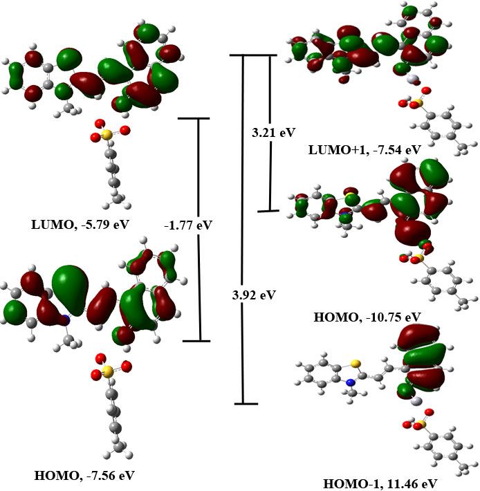
Chemosensors 2019, 7, 35                                                                         2 of 19

their effects on the nervous, digestive and immune systems, and on lungs, kidneys, skin, and eyes
[17]. Exposure to even a small concentration of mercury can produce a number of negative health
problems like minamata disease [18–20]. The world health organization considers the pollution
caused by mercury among the top ten environmental problems that affect the health of humans
seriously [16,21]. Owing to the hazardous effect of the presence of mercuric ions in water, it is
imperative to develop sensitive and selective methods for easier detection of mercuric ions in water.
Instrumental techniques such as atomic absorption spectrometry, inductively coupled plasma atomic
emission spectroscopy (ICP‐AES) etc. are available for the detection and determination of mercuric
ions. However, instrumental techniques are expensive and non‐portable and require collection and
transportation of the samples for evaluation [22–24]. The monitoring of contaminated sites requires
on‐site evaluation of samples, which is difficult to achieve with bulky and expensive
instrumentations. Therefore, there is a need to develop simple, easy and portable techniques for the
detection of mercuric ions in natural water sources such as lakes and rivers. The drawback associated
with instrumentation techniques may be rectified by the use of optical sensors, which are simple,
portable and display optical signal in the presence of analyte [25]. In most of the analysis, the sensor
molecule is the most expensive chemical species consumed during the operation, which increases the
cost of the procedure. Therefore, there is a need to develop sensors, which can be reused for multiple
assays. However, most of the sensors reported in the literature require harsh conditions for
regeneration, which either leads to a change in the composition of the sensing material or lead to a
further increase in pollution [5,26,27]. In this context, light responsive sensing materials are gaining
attention as the light of a suitable wavelength can be used for their regeneration without the need for
any chemical additive [28]. Among a variety of optical sensors available in the literature, the
merocyanine form of spiropyran represent a family of photo‐responsive molecules, which rapidly
and sensitively undergoes a change in color in response to coordination with an analyte [28,29]. The
spiro form, usually displays no color (non‐polar form), while the merocyanine form displays an
intense color (highly polar). Due to the high polarity of the merocyanine form and the presence of the
phenolic oxygen atom, it usually interacts with anions or cations. In addition, the merocyanine form
also displays an intense color due to the formation of H‐ or J‐ aggregates [30]. The formation or
disruption of aggregation may further lead to a change in color or emission [31,32]. If this change in
the aggregation properties and in turn the optical signal is induced by a metal ion, the phenomenon
may be used for the detection purpose. Further, the polar nature of the merocyanine form improves
the solubility of the sensor in the water. However, the merocyanine forms are usually unstable and
easily               transforms                in               the              spiro              form
[33–35]. Therefore, the merocyanine form as a p‐toluenesulfonate salt was synthesized and evaluated
for the detection of highly toxic mercuric ions. The change in color or fluorescence signal due to the
complex formation between the metal ion and the merocyanine form can be used for the
determination of low concentration of analyte with the help of UV‐visible or fluorescence
spectroscopy. In addition, the change in color intensity can be analyzed using the digital image based
colorimetric method, which is receiving increased attention owing to easy, low cost and portable
analysis of a variety of samples [36–38]. The method only requires a change in color upon addition
of an analyte [36]. Therefore, the use of the merocyanine form can further help in the detection of an
analyte through the digital image analysis.

2. Materials and Methods
    The NMR spectra were recorded using a 400 MHz Jeol NMR ECX 400 NMR spectrometer (Jeol
USA, Inc., Peabody, MA, USA) in deuterated dimethyl sulfoxide (DMSO‐d6). The UV‐Visible studies
were performed on an Ocean Optics USB 4000 UV–visible spectrometer (Ocean Optics, Dunedin, FL,
USA). Cary Eclipse Fluorescence spectrophotometer was used to record the fluorescence spectra
keeping slit widths at 20 nm. Hydrodynamic Size (d, nm) were recorded on the Malvern ZetaSizer
NanoZS DLS Instrument (Malvern Pananlytical, Malvern, UK).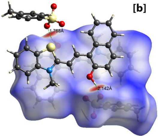
Chemosensors 2019, 7, 35                                                                          3 of 19

2.1. Synthesis
      The synthesis details of the receptor have been reported earlier [30].

2.2. UV‐Visible Studies
     A solution (2.2 mL) of receptor 1 (20 μM) in water buffered at pH 7.6 using 1.0 mM 4‐(2‐
hydroxyethyl)‐1‐piperazineethanesulfonic acid (HEPES) was taken in a quartz cuvette to record the
UV‐Visible spectrum using an Ocean Optics UV‐Visible spectrometer. A solution of the Hg2+ ions in
water at pH 7.6 (1.0 mM HEPES) was gradually added to the cuvette. The UV‐Visible spectra were
recorded after each addition.

2.3. Procedure for Fluorescence Studies
     A solution (2.2 mL) of receptor 1 (20 μM, pH 7.6, 1.0 mM HEPES in water) was taken in a quartz
cuvette to record the fluorescence spectrum using the Cary Eclipse Fluorescence Spectrophotometer.
A solution of the Hg2+ ions in water at pH 7.6 (1.0 mM HEPES) was gradually added to the cuvette.
The fluorescence spectra were recorded after each addition using 365 nm excitation wavelength and
20 nm slit widths (both).

2.4. Color Intensity Measurement Studies
     A solution (3.0 mL) of receptor 1 (40 μM, pH 7.6, 1.0 mM HEPES in water) was taken in vials
and an increasing concentration of mercuric ion solution was added. The color photograph of the
solution was taken using a smartphone device (Realme 3 pro with a 16MP camera). The photograph
was analyzed for intensity using the ImageJ software [39].
     Crystals: Suitable crystal was mounted at 297 K for X‐ray diffraction and the data was recorded
using the Xcalibur, Sapphire3 diffractometer. The details of crystal data, collection and structure
refinement parameters for 1 are given in Table S1. The ShelXD/duel space program with Olex2 [40]
GUI was used to solve the structure, which was further refined using the ShelXL/least square
program [41]. The non‐hydrogen atoms were refined anisotropically, while the hydrogen atoms like
C‐H (aromatic), ‐CH2 and ‐CH3 were placed at appropriate positions (C‐H = 0.93 Å, ‐CH2 = 0.97 Å, ‐
CH3 = 0.96 Å and treated using a riding model keeping Uiso (H 4C‐H and ‐CH2) = 1.2Ueq(C), Uiso (H 4‐
CH3) = 1.5Ueq(C). The ‐CH3 groups were treated as ideal rotary groups during refinement. The O‐H
group hydrogen atom in the structures was located at O‐H = 0.82 Å and refined freely. The figures
used in this paper were obtained using the Mercury software [42].
     Computations: The entire computational work was performed by using the Gaussian 09 A02
software suite [43]. The initial geometries of 1 or 1‐Hg2+ complexes were constructed using the Gauss
View 05 and optimized using the DFT/PBE1PBE/6‐31+G(d) method, while the LANL2DZ basis set
was used for mercury during the optimization of the complex geometries. The different stereoisomers
of 1 were constructed through the rotation of three bonds that link the indole unit to the phenolic
unit. The three bonds may take either a cis or a trans orientation. Based on the cis or trans orientation
of the three bonds, the stereoisomers may be classified as CTC, TTC, TTT and CTT (Figure S4). The
four stereoisomer CCC, CCT, TCC and TCT were not optimized due to their comparative low
stability. The frequency calculations indicated the presence of a local minimum state. The most stable
geometry was used to obtain the electronic excitation parameters using the DFT/PBE1PBE/6‐31+G(d)
method for 1 and DFT/PBE1PBE/6‐31+G(d)‐LANL2DZ method for the complex.

3. Results and Discussion
     Synthesis: Receptor 1 was synthesized by refluxing 2,3‐dimethylbenzothiazolium p‐
toluenesulfonate salt with 2‐hydroxy‐1‐naphthaldehyde in ethanol in the presence of the catalytic
amount of piperidine (Scheme 1). The product was characterized using IR, 1H‐, 13C‐NMR and HR‐MS
techniques as well as single crystal X‐ray crystallography (Figures S1–S3).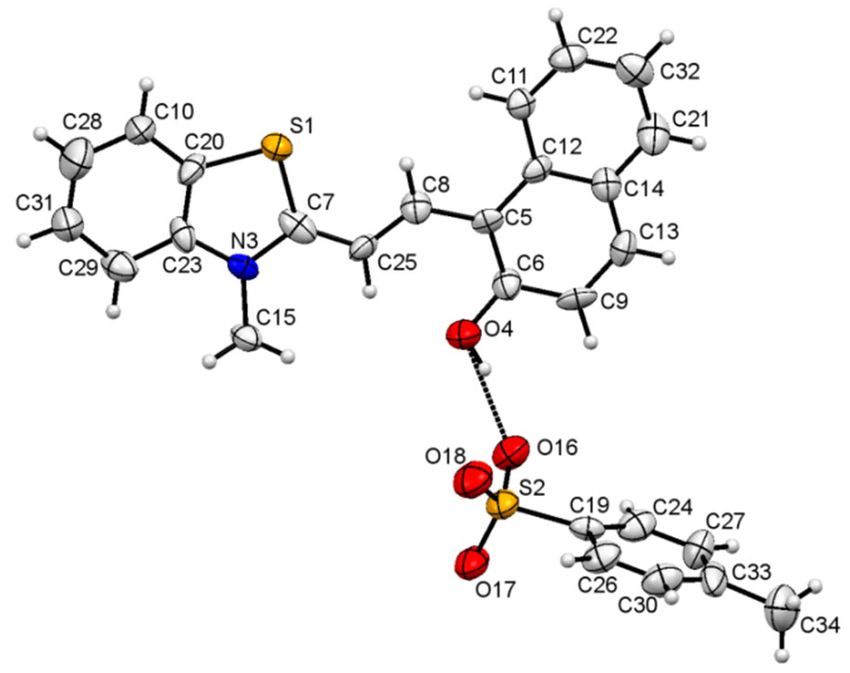
Chemosensors 2019, 7, 35                                                                                  4 of 19

                                      S
                                                                                    S
                                      N            HO
                                               +                   Ethanol
                                                                                    N        HO
                                               OHC
                                       SO 3-                       Piperidine
                                                                                     SO 3-

                               Scheme 1. The synthetic scheme for the preparation of 1.

     Crystallography: The crystals suitable for the X‐ray diffraction were grown from a solution of 1
in ethanol. The crystal parameters are listed in Table S1. The asymmetric unit displayed the presence
of TTC stereoisomer of the merocyanine form of 1 linked to a molecule of the p‐toluenesulfonate
group (Figures 1 and S4). The strong short contact between the oxygen atom of the p‐toluenesulfonate
group and the sulfur atom was also observed (Figure S5). In addition, the oxygen atom of the p‐
toluenesulfonate group was found to interact strongly with the aromatic C‐H group (Figure S6, Table
1). The crystal packing diagram revealed the alternate arrangement of the p‐toluenesulfonate and
merocyanine unit, which leads to the formation of chains that propagate along [100] planes (Figures
2 and S7). The crystal packing revealed the presence of several short intermolecular contacts of O‐
H...O, O‐H…S, C‐H…O types (Table 1, Figures S8 and S9).

      Figure 1. An ORTEP view [42] of the asymmetric unit for 1 showing the TTC unit linked to the p‐
      toluenesulfonate moiety through the H‐bond. Displacement ellipsoids are at 50% probability.

                                       Table 1. Hydrogen‐bond geometry (Å, °).

                              D—H∙∙∙A                    D—H           H∙∙∙A       D∙∙∙A      D—H∙∙∙A
                             O4—H4∙∙∙S2i                0.92 (9)     2.66 (10)   3.520 (6)    155.0 (8)
                            O4—H4∙∙∙O16i                0.92 (9)     1.65 (9)    2.571 (7)    176.1 (9)
                           C15—H15B∙∙∙O17ii               0.96         2.54      3.433 (9)     154.4
                            C25—H25∙∙∙O4                  0.93         2.11      2.747 (9)     124.9
                           C29—H29∙∙∙O17ii                0.93         2.40      3.332 (9)     178.0
                               Symmetry codes: (i) −x + 2, −y + 2, −z; (ii) x, −y + 3/2, z−1/2.

     The Crystal Explorer software was further used to investigate the intermolecular interactions
present in 1 through the Hirshfeld surface analysis [44]. The dnorm function, which considers the nuclei
interior (di), the exterior (de) and Van der Waal’s radii (rvdw) were used to map the Hirshfeld surface.
The big red spots on the Hirshfeld surface indicate strong short intermolecular contacts like O…H‐O
and O…S‐H. In addition, the π…π stacking, C‐H…π, and C‐H…O type interactions were also observed,
which links the chains together forming aggregated chains of molecular units (Figure 3).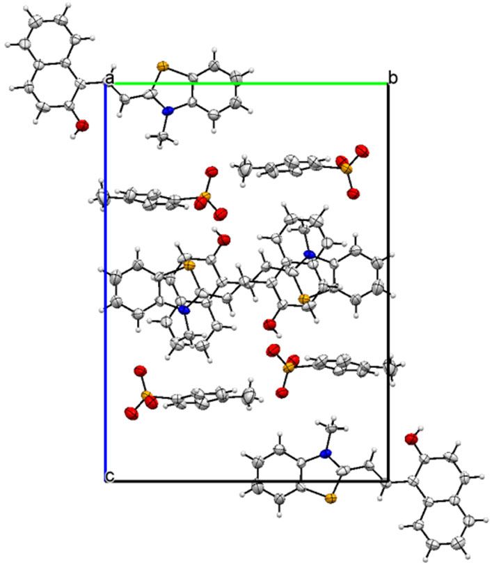
Chemosensors 2019, 7, 35                                                                                  5 of 19

      Figure 2. The crystal packing diagram of 1 viewed along axis a with displacement ellipsoid at 50%
      probability.

      Figure 3. Hirshfeld surface analysis of 1 showing intermolecular short contacts. (a) Hirshfeld surface
      showing big red spots indicating strong intermolecular contacts, (b) Hirshfeld surface showing O‐
      H…O interactions.

     The 2D‐Fingerprint plots obtained using the Crystal Explorer program [44,45] were used to
quantitatively estimate the contribution of different type of interactions to the total Hirshfeld surface
(Figures 4a and 5). The intermolecular O…H interactions, as expected, contributed significantly
(21.0%) to the total Hirshfeld surface (Figure 4b). However, the major contribution to the Hirshfeld
surface area emanates from π…π interactions (H…H: 44.7% and C…C 6.6%) (Figure S10). The C…H
interactions also contributed significantly to the total surface area (22.0 %) (Figure S11a), while the
other interactions (C…N: 1.4%, S…H: 0.9%, C…O: 0.1%, O…O: 0.3% and S…C: 3.0%) contributed to a
smaller extent to the total Hirshfeld surface (Figures 5 and S11b–S13). However, the fingerprint plot
indicated that the S…O interactions were insignificant to measure (less than 0.1%) (Table S2).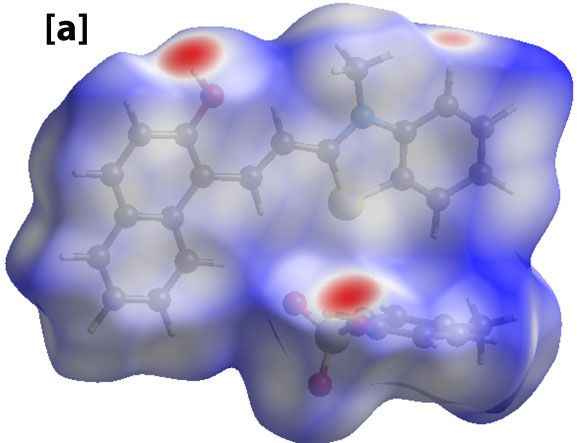
Chemosensors 2019, 7, 35 6 of 19
Figure 4. Two‐
dimensional (2D)‐fingerprint plot of 1 showing (a) complete Hirshfeld surface;
(b) O‐H…O short contacts.
S-H S-C O-O
O-H C-O C-N
H-H C-H
1
0 10 20 30 40 50 60 70 80 90
%
Figure 5. The percentage contribution of different intermolecular contacts to the total Hirshfeld
surface.
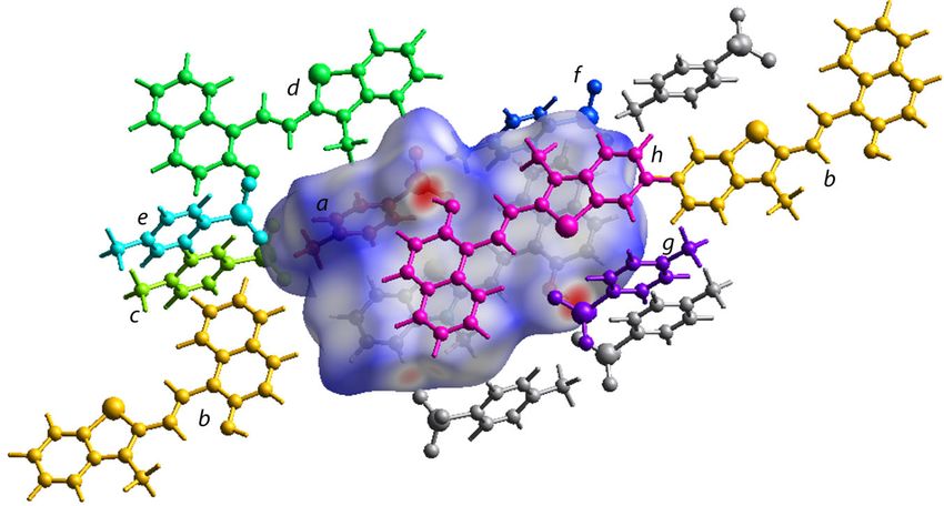
The TONTO program in the Crystal Explorer software (B3LYP/6‐31G(d,p) method was further
used to estimate the energies between different molecular pairs like the central merocyanine unit and
molecules surrounding it (Figures 6 and S14) [44]. The energies are listed in Table 2. The Crystal
Explorer program provides the total interaction energies along with individual energy components
such as electronic, dispersion, repulsion, and polarization energy. The calculations indicated
−14.4 kJ/mol as total interaction energies between the p‐toluenesulfonate moiety (a) and the
merocyanine fragment (central unit) interacting with each other through the O…S and C‐H…O type
short contacts. The central merocyanine unit and the h moiety interacted using π…π stacking
interactions to contribute −80 kJ/mol towards the stabilization of the crystal lattice. The O…H‐O type
H‐bond between the merocyanine unit and p‐toluenesulfonate contributed −14.8 kJ/mol towards the
stabilization of the crystal lattice. The interaction energies between other molecular pairs are listed in
Table 2 (Figures 6 and S14).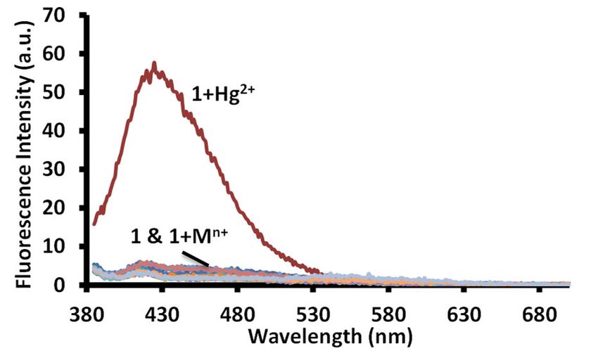
Chemosensors 2019, 7, 35                                                                                            7 of 19

      Figure 6. The Hirshfeld surface incorporating the asymmetric unit showing the interactions with the
      neighboring molecular units in the crystal packing. Different molecular units around the central
      molecule are labelled from a‐h.

      Table 2. The energies of interaction (kJ/mol) between the molecular pair calculated using the Crystal
      Explorer (TONTO) program using the B3LYP/6‐31G(d,p) method.

              Frag.    N          Symop               R       E_ele    E_pol      E_dis     E_rep      E_tot
                a      1              ‐             5.42       −5.8     −4.3       −30        34       −14.4
                b      1           x, y, z          15.3       −0.4     −0.2       −9.2       7.2      −4.1
                c      1              ‐             13.17      0.4      −0.1       −0.3        0        0.2
                d      1    x, −y + 0.5, z + 0.5    12.3       −0.1     −0.1       −0.9        0        −1
                e      1              ‐             12.5       −0.1     −0.2       −0.6        0       −0.8
                f      1              ‐             9.07       −1.3     −0.9       −13        7.8      −8.5
                g      1              ‐              7.8      −49.8    −10.1      −13.2       92       −14.8
                h      1         −x, −y, −z         4.07      −22.9     −9.1      −113.6     80.7       −80

3.1. Naked Eye Detection
      Due to the polar nature of the merocyanine unit along with the presence of p‐toluenesulfonate
as a counter anion, 1 was screened for affinity towards toxic metal ions in water. Solutions of different
metal ions and receptors were prepared in water buffered at pH 7.6 using 1.0 mM HEPES. An
equivalent solution of different metal ions was mixed with a solution of 1 in water (pH 7.6,
1.0 mM HEPES). A color change to colorless was observed in a solution containing mercuric ions,
while the solutions containing other metal ions displayed a faint change in color or a color change to
light yellow, which indicated that 1 can be used for the visual detection of mercuric ions in water
(Figure 7).

      Figure 7. Color change in the solutions of receptor 1 in water (pH = 7.6, 1.0 mM HEPES) upon addition
      of acetate salts of various metal ions. [1] = 20 μM. From left to right, A = Free, B = Hg2+, C = Al3+, D =
      Cr3+, E = Fe3+, F = Cu2+, G = Rb+, H = Sm3+, I = Zn2+, J = K+, K = Gd3+, L = Pb2+, M = Ca2+, N = Ni2+, O = Cd2+,
      P = Fe2+, Q= Mg2+, R = Pd2+, S = Na+, T = Cs+, U = Li+, V = Ba2+, W = Co2+, X = Sr2+.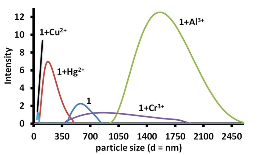
Chemosensors 2019, 7, 35                                                                                       8 of 19

3.2. UV‐Visible Studies
      The equimolar solutions of different metal ions and 1 in water (pH 7.6, 1.0 mM HEPES) were
analyzed using the UV‐Visible spectroscopy. The absorption spectra of 1 in water (pH 7.6, 1.0 mM
HEPES) displayed the presence of two bands (λmax = 570 nm and λmax = 455 nm). The solution of
mercuric ion to 1 led the disappearance of both the bands (λmax = 570 nm and λmax = 455 nm), with the
appearance of a new absorption band with maxima at 380 nm. The addition of other metal ions (Al3+,
Fe3+, Cu2, and Cr3+) to the solutions of 1, led to a decrease in the absorption band at 570 nm and a small
increase in the absorption band at 455 nm (Figures 8 and S15).

                                           1

                                      0.8
                                                                                1 & 1+Mn+
                              Absorbance

                                      0.6
                                                     1+Hg2+
                                      0.4                                           1+Al3+
                                                                 1+Cu2+
                                      0.2                                           1+Fe3+
                                                                    1+Cr3+
                                           0
                                               300   350   400    450 500 550 600    650     700
                                                                  Wavelength(nm)

      Figure 8. Change in absorption spectra of solutions of receptor 1 in water (pH = 7.6, 1.0 mM HEPES)
      upon addition of acetate salts of different metal ions. [1] 20 μM = [Mn+] = Hg2+, Na+, K+, Li+, Cr3+, Al3+,
      Fe3+, Mn2+, Ni2+, Pb2+, Zn2+, Co2+, Cu2+, Cs+, Ba2+, Sr2+ ions.

     A Job’s plot experiment was performed to determine the stoichiometry of the complex between
1 and the mercuric ions, which displayed no clear stoichiometry. Mass spectra of a solution
containing 1 and the mercuric ion was recorded in acetonitrile, it produced a strong peak at 657.1058
(Figure S16). The mass peak corresponds to C24H25HgNO6S+ (m/z: 657.1109), which correspond to a
molecule of the merocyanine form linked to one mercuric ion having two acetate ions and a water
molecule to complete the coordination sphere. The mass spectra indicated the formation of a 1:1
complex stoichiometry. In addition, the detection of mercuric ion by 1 was performed in the presence
of one equivalent concentration of different metal ions, which indicated no significant interference
(Figures S17–S19). The interference experiments indicated that mercury ions can be detected in water
even in the presence of other metal ions (Figures S17–S19).
     In order to further investigate the formation of a complex between 1 and metal ion, the solutions
of 1 were titrated with Hg2+, Fe3+, Al3+, and Cu2+ ions in water at pH 7.6 (1.0 mM HEPES). The
incremental addition of a solution of 1 with the Hg2+ ion produced a gradual decrease in the
absorbance of the bands at ~450 nm and ~570 nm with simulataneous appearance of a new band at
~380 nm (Figures 9 and S20). The gradual addition of a solution of copper ions to a solution of 1 in
the water at pH 7.6 (1.0 mM HEPES) produced a small decrease in the absorption band at ~455 nm
and a significant decrease in the absorption band at ~570 nm (Figure S21). However, no additional
peak appeared in the absorption spectra. The addition of a solution of Al3+, Cr3+ or Fe3+ ions to a
solution of 1 in water (pH 7.6, 1.0 mM HEPES) produced a gradual decrease in the intensity of the
band ~580 nm, while no significant change in the absorption intensity at ~455 nm was observed
(Figures S22–S24). The titration results were further analyzed for the calculations of the association
constant between 1 and the metal ions using the HypSpec program (Figures 10 and S25–S28) [46].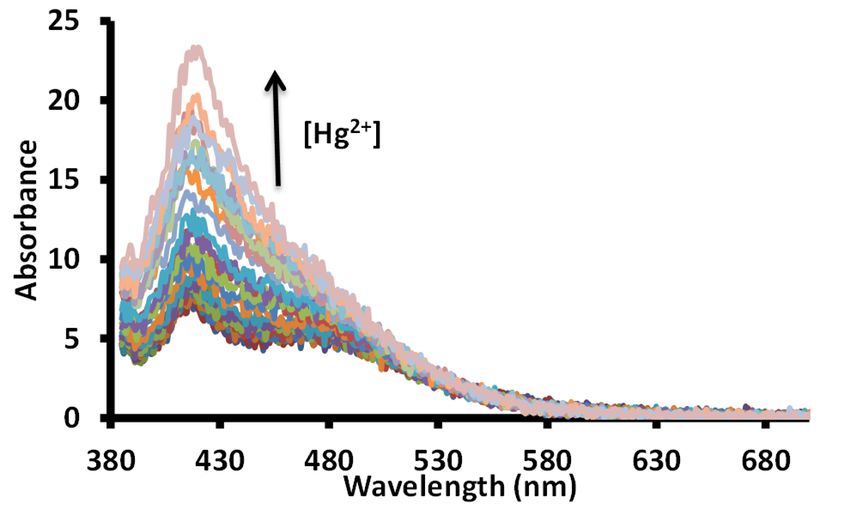
Chemosensors 2019, 7, 35                                                                                      9 of 19

                                     0.7
                                     0.6
                                     0.5

                            Absorbance
                                     0.4
                                                        [Hg2+]
                                     0.3
                                     0.2
                                     0.1
                                            0
                                                  300        350    400   450 500 550 600         650   700
                                                                          Wavelength (nm)

      Figure 9. Change in the absorption spectra of a solution of receptor 1 in water (pH = 7.6, 1.0 mM
      HEPES) upon incremental addition of acetate salts of mercuric ions. The up arrow indicates an
      increase in absorption band intensity, while a down arrow indicates a decrease in absorption band
      intensity with an increase in mercuric ion concentration; [1] = 20 μM; [Hg2+] = 0–13.63 μM.

     The HypSpec program [46] utilized different binding equilibria between the host and the guest
species to calculate the association constant. Therefore, different binding equilibria were used to fit
the observed absorbance value with the calculated absorbance value using the HypSpec program
(Figures S10 and S25–S28). The calculations that utilized 1:1 (Host:Guest) binding equilibria produced
the best correlation between the observed and calculated absorbance values and yield association
constant shown in Table 3.

                                            0.25

                                                  0.2
                                     Absorbance

                                            0.15

                                                  0.1
                                                                   Observed Absorbance
                                            0.05
                                                                   Calculated Absorbance
                                                   0
                                                         0         0.000003   0.000006 0.000009   0.000012
                                                                              [Hg2+] μM

      Figure 10. A correlation between the observed absorbance and absorbance value calculated using the
      HypSpec program for a titration between 1 and Hg2+ ions with 1:1 (H:G) binding stoichiometry.

      Table 3. The binding constant value obtained for a 1:1 (H:G) binding stoichiometry and changes
      observed at a different wavelength for 1 with different metal ions.

                                 Metal                            Logβ11          Change in λmax (nm) at
                                 Hg2+                         5.2480 ± 0.0229         380, 450, 570
                                 Cu2+                         5.0172 ± 0.0193           455, 564
                                 Al3+                         4.8992 ± 0.0504              563
                                 Cr3+                         4.8949 ± 0.0075              564
                                  Fe3+                       4.59582 ± 0.0307              563

3.3. Fluorescence Studies
     The aggregated solution of the merocyanine form is known to display a change in fluorescence
intensity upon addition of an analyte. Therefore, equimolar solutions of 1 and metal ions were
investigated for change in emission spectra using 570 nm, 450 nm, and 365 nm excitation wavelengths
in the water at pH 7.6 (1.0 mM HEPES). A very faint fluorescence signal was observed using 450 nm
and 570 nm excitation wavelengths in a solution of 1 and 1 with metal ions. However, an equimolar
solution of 1 and mercuric ion displayed a strong emission band at 425 nm with a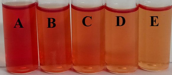
Chemosensors 2019, 7, 35                                                                                        10 of 19

45 nm Stokes shift using a 365 nm excitation wavelength (Figures 11 and S29). The equimolar solution
of 1 and mercuric ion displayed a 27 fold enhancement in the fluorescence intensity in comparison to
the fluorescence intensity displayed by a solution of 1 in water (Figure 11). However, no change in
the fluorescence intensity was observed for solutions containing 1 and other metal ions.
      Further, a titration experiment was conducted between a solution of 1 and mercuric ions in water
at pH 7.6 (1.0 mM HEPES) using a 365 nm excitation wavelength at 20 nm slit width. The gradual
addition of a solution of mercuric ions produced a gradual increase in the fluorescence intensity at
425 nm (Figure 12).

      Figure 11. Change in fluorescence spectra of solutions of receptor 1 in water (pH = 7.6, 1.0 mM HEPES)
      upon addition of acetate salts of different metal ions. [1] = 20 μM = [Mn+] = Hg2+, Na+, K+, Li+, Cr3+, Al3+,
      Fe3+, Mn2+, Ni2+, Pb2+, Zn2+, Co2+, Cu2+, Cs+, Ba2+, Sr2+ ions.

      Figure 12. Change in fluorescence spectra of a solution of receptor 1 in water (pH=7.6, 1.0 mM HEPES)
      upon incremental addition of acetate salts of mercuric ions. The up arrow indicate an increase in
      intensity with an increase in mercuric ion concentration; [1] = 20 μΜ; [Hg2+] = 0–0.67 μΜ.

3.4. DLS Studies
     The solid‐state solution of 1 displayed the presence of networks of molecular chains linked
through H‐bonds. In addition, the solution of 1 displayed an absorption band near 570 nm, which
indicated that it may be present in the aggregated form (J‐aggregation) [32]. Therefore, dynamic light
scattering experiments were performed for solutions of free 1 and 1 containing different metal ions,
which produced a change in absorption spectra. A solution of 1 displayed a mean particle size of 535
nm. The addition of one equivalent mercuric ion to a solution of 1 produced a decrease in the mean
particle size of 168 nm. A similar decrease in the particle size was also observed in an equimolar
solution of copper ions and 1. However, a solution of aluminum (~1594 nm) and chromium (851 nm)
displayed an increase in the mean particle size, which indicated that the decrease in the absorbance
at 455 nm and 470 nm is due to dis‐aggregation, while a decrease in the absorbance at 470 nm only,
indicate stronger aggregation. The experiment further indicates that mercury and copper ions cause
dis‐aggregation of 1, while ferric, aluminum and chromium ions induce aggregation in 1 (Figure 13).
Chemosensors 2019, 7, 35 11 of 19
Figure 13. The particle size observed in a solution of 1, 1‐Hg2+ (1:1), 1‐Cr3+ (1:1), 1‐Al3+ (1:1) and 1‐Cu2+
(1:1) in water; [1] = [Hg2+] = [Cr3+] = [Al3+] = [Cu2+] = 1.02 mM.
3.5. NMR Studies
In order to investigate the formation of a complex between the mercuric ions and 1, the 1H‐NMR
spectra of 1, 1‐Hg2+ and 1‐Al3+ were recorded in DMSO‐d6 (Figures 14 and S30). Due to the
paramagnetic effect associated with the copper, ferric and chromium ion solutions, the 1H‐NMR of
their complex was not recorded. The 1H‐NMR of 1 indicated the alkene proton (H7 and H8) at δ8.59
and δ8.18 ppm (Figure 14). The OH group signal was observed at δ11.79 ppm. The NCH3 group signal
was observed at δ4.24 ppm, which indicated the presence of the merocyanine form of 1 in the
solution. The addition of mercuric ion to a solution of 1 produced an upfield shift in the signal due
to aromatic and aliphatic protons. The signal due to proton H1 shifted from δ7.35 ppm to δ6.57 ppm,
which indicated the absence of hydrogen atom attached to the phenolic oxygen atom. The signal due
to proton H9 shifted from δ8.39 to δ6.97 ppm, which indicated a reduction in the positive charge on
the nitrogen atom. Similarly, signals due to other protons in the indole ring also shielded owing to a
reduction in the positive charge on the nitrogen atom. The N‐CH3 signal also shielded and shifted
from δ4.24 ppm to δ2.86 ppm upon addition of the mercuric ion (Figure S30). The mass spectra
produced no peak due to a dimerized form of 1. The 1H‐NMR also indicated the absence of the closed
form of 1. Therefore, the analysis of 1HNMR indicated the formation of a complex, where the mercuric
ion is linked to the quinoidal form of 1 through the phenolic oxygen atom [47]. The 1H‐NMR of 1‐Al3+
complex indicated the absence of a significant shift in the signal due to aromatic or aliphatic protons
(Figures S31 and S32). A small and insignificant shift in the signals due to different protons indicated
that the complex formation between the aluminum ion and 1 may lead to a change in the aggregation
state only.
1+Hg2+
5 4
6 3
12 7 13
S 2 6, 8 14
11 7 12 2 11 1
3 5 10 4 1
10 8 HO 1 9
N
9 13
O3 S
14
8.5 8 7.5 7 6.5
ppm
Figure 14. Partial 1H‐NMR spectra of 1 and 1‐Hg2+ in DMSO‐d6 recorded on a 400 MHz instrument
showing a comparison in the aromatic region.Chemosensors 2019, 7, 35 12 of 19
3.6. Practical Utility
For any practical utility of 1 for the detection of mercuric ions, it is imperative to determine the
limit of detection value. Therefore, the limit of the detection value of 1 towards mercuric ions was
determined using UV‐Visible and fluorescence spectroscopies with the help of the 3σ/m equation. A
straight line curve was observed between the absorbance (570 nm) and the concentration of mercuric
ions. Similarly, a straight line curve was observed between the fluorescence intensity at 424 nm and
the mercuric ion concentration (Figures 15 and S33). The UV‐Visible data yielded 0.32 μM as the limit
of detection value for 1 towards mercuric ions, while 67.8 nM limit of detection values for 1 towards
mercuric ion was observed using fluorescence data.
0.4
0.35
0.3
Absorbance
0.25
0.2
0.15 y = ‐0.0292x + 0.3571
R² = 0.9978
0.1
SD = 0.0030
0.05
0
0 1 2 3 4 5 6 7
[Hg2+] μM
Figure 15. The determination of limit of the detection value of 1 towards mercuric ions using ultra
violet (UV)‐Visible spectroscopy.
The detection limit was further established using the color intensity measurement method. For
on‐field utilization of any sensor for the detection of toxic metal ion, it is essential to carry out the
analysis using simple devices. Therefore, color photographs of solutions taken using a smartphone
followed by their color intensity analysis with the software can be useful for on field measurement
of toxic metal ion concentration in water samples (Figure 16). The solutions of 1 containing a different
concentration of mercuric ions were prepared. The digital images of the solutions were analyzed
using the ImageJ software (Figure 16). The pixel intensity of the solution versus the concentration of
mercuric ion was plotted, which yielded a straight line. The straight line plot yielded 89.4 nM as the
limit of the detection value of 1 towards mercuric ions. The limit of detection value observed through
the color intensity measurement was found to be better than obtained using the UV‐visible
spectroscopy.
120
100
80
Intensity
60 y = 19.736x + 64.78
40 R² = 0.999
20
0
0 0.5 1 1.5 2 2.5
[Hg2+] μM
Figure 16. The determination of limit of detection value of 1 towards mercuric ions using the solution
intensity method. (Left) Concentration of Hg2+ ion in: A = 0.0 μM; B = 0.53 μM; C = 1.06 μM;
D = 1.58 μM; E = 2.10 μM. (Right) A graph showing the change in pixel intensity of the solution with
an increase in the mercury ion concentration.Chemosensors 2019, 7, 35 13 of 19
Further, filter paper test strips were prepared from the Whatman filter paper and dipped into a
solution of 1 in acetonitrile. The filter paper strips after drying in the air were dipped in the solutions
of different metal ions. A filter paper strip dipped in a solution of mercuric ion decolorized, while
filter paper strips dipped in the solutions of ferric and chromium ions displayed a yellow color. A
small, insignificant change in the color was observed on filter paper strips dipped in solutions
containing other metal ions (Figure 17). The experiment indicated that 1 can be used for the detection
of mercuric ions in water.
Figure 17. Color change on paper strips coated with the receptor 1, dipped in the solutions of acetate
salts of various metal ions. [1] = 20 μM. From left to right, A = Free, B = Hg2+, C = Al3+, D = Cr3+,
E = Fe3+, F = Cu2+, G = Rb+, H = Sm3+, I = Zn2+, J = K+, K = Gd3+, L = Pb2+, M = Ca2+, N = Ni2+, O = Cd2+,
P = Fe2+, Q = Mg2+, R = Pd2+, S = Na+, T = Cs+, U = Li+, V= Ba2+, W = Co2+, X = Sr2+.
3.7. Computational Studies
In order to understand the complex formation between 1 and mercuric ions, the
PBE1PBE(PBE0)/6‐31+G(d) method was used with the Gaussian program suite [43]. Due to the
presence of a number of short contacts in 1, the PBE0 method was chosen as it yields good results
with noncovalent interactions during the calculations [48]. The geometries of 1 in the TTT, TTC, CTC
and CTT stereo‐isomeric forms were optimized. The calculations indicated that the TTC form is the
most stable stereo‐isomeric of 1 (Table 4, Figures 18 and S34).
Figure 18. The DFT/PBE1PBE/6‐31G(d)/LANL2DZ optimized geometries of the most stable form of 1
and its complex with mercuric ion. (a) the geometry of the TTC form linked to a p‐toluenesulfonate
group, (b) the geometry of the TTC‐Hg2+ complex.Chemosensors 2019, 7, 35 14 of 19
Table 4. The calculated total and relative energies (kcal/mol) calculated using the PBE1PBE/631+G(d)
method.
Stereo‐Isomer E1a E2 b E3 c Erel = ETTC − ESId E1+Hg Ercf ΔE = E1−Hg2+ − (E3 + EHg2+)
TTC −814,597.26 −814,854.47 −1,376,038.65 0 −1,402,460.35 0 −195.90
CTT −814,599.01 −814,849.28 −1,376,032.66 5.98 −1,402,457.10 3.24 −198.64
CTC −814,602.62 −814,851.30 −1,376,032.18 6.47 −1,402,457.77 2.57 −199.79
TTT −814,595.80 −814,852.95 −1,376,031.82 6.82 −1,402,460.04 0.31 −202.41
aisomers shown in Figure S35; b isomer shown in Figure S36; c isomers shown in Figures 18 and S34
dESI is the energy of different stereoisomers of 1. f Erc is the relative energy with respect to the energy
of the TTC‐Hg complex.
The DFT/PBE1PBE/6‐31+G(d)/LANL2DZ method was further used to optimize the geometry of
the complex between different stereoisomers of 1 and mercuric ion. The different geometries of the
complex with and without p‐toluenesulfonate were optimized. The geometries having the p‐
toluenesulfonate group as the coordinating group were observed to be more stable than the
geometries, which were optimized without this moiety. However, it may be interacting weakly with
the mercuric ion. Further, the position of the hydrogen atom that links the p‐toluenesulfonate group
and the merocyanine form was also established using DFT calculations. For, the TTC isomer, the
combined energy of the p‐toluenesulfonic acid and the unprotonated form of merocyanine (TTC) was
compared with the combined energy of the p‐toluene sulfonate and protonated form of the
merocyanine (TTC+H), which indicated that the former is more stable than the latter by
−63.84 kcal/mol. Further, a comparison of the energy of the different complex geometry indicated that
the TTC isomer forms the most stable complex with the mercuric ion (Table 4, Figures S35–S37). In
addition, the combined energy of the different stereoisomer of 1 and Hg2+ ion was compared with the
energy of the stereoisomer‐Hg2+ complex, which indicated higher stability of the complex in
comparison to the reactants (Table 4). Further, calculations indicated that the TTT isomer should form
the complex much more readily than the other stereoisomers of 1 (Table 4, Figures S35–S37). The
PBE1PBE/6‐31+G(d) optimized the geometry of the most stable stereoisomer of 1 (TTC) was further
used for the calculation of excitation parameters using the TD‐DFT/PBE1PBE/6‐31+G(d) method. The
calculation indicated that the transition between HOMO to LUMO orbitals (So to S1) is responsible
for the observed absorption band in 1 (Figure 19, Table S3). The most stable geometry of the 1‐Hg
complex was used to calculate the excitation parameters using the TD‐DFT/PBE1PBE/6‐31+G(d)
method, which suggested that HOMO to LUMO+1 and HOMO‐1 to LUMO+1 orbitals are responsible
for the observed singlet electronic observed in 1 (Figure 19). The electronic excitation parameters are
given in Table S3. The TD‐DFT calculations indicated that there is an increase in the ground state to
the excited state gap, which causes a hypsochromic shift.Chemosensors 2019, 7, 35 15 of 19
Figure 19. The TD‐DFT/PBE1PBE/6‐31+G(d)/LANL2DZ calculated energy diagram of 1 and 1‐Hg2+
complex showing main orbitals involved in the transition.
4. Conclusions
In summary, the structure of the merocyanine form was established using the single crystal X‐
ray crystallography to reveal extensive H‐bonding that led to the formation of aggregates. The energy
of the interactions was determined. The merocyanine form detected the presence of mercuric ions in
water through the disaggregation mechanism and displayed a change in color visible to the naked
eye (pink to colorless). The trivalent metal ions like chromium, aluminum, and ferric ions caused
further aggregation of the merocyanine form. The association constant values were calculated, which
indicated the formation of a complex between the mercuric ion and the merocyanine form. The lower
value of the association constant was observed with trivalent metal and copper ions. The complex
between the receptor and mercuric ion displayed a fluorescence response. Both UV‐visible and
fluorescence studies provided a good limit of the detection value of the receptor towards mercuric
ions. Further, the limit of the detection value was obtained from a solution of the receptor and
mercuric ion using the pixel intensity analysis, which provided a better limit of detection value in
comparison to the UV‐Visible spectroscopic analysis. It was demonstrated that the image pixel
analysis can provide a better limit of the detection value of 1 for mercuric ions. DLS studiesChemosensors 2019, 7, 35 16 of 19 demonstrated the disaggregation of the merocyanine form in the presence of the mercuric ion. The 1H‐NMR further indicated the formation of a complex between the merocyanine form and the mercuric ion. The DFT studies indicated that the TTC form is the most stable stereoisomeric form of the receptor. The TD‐DFT studies indicated that the addition of the mercuric ion increases HOMO and LUMO gap in the receptor, which support the experimental results. Supplementary Materials: The following are available online at www.mdpi.com/xxx/s1, Figure S1: The 1H‐ NMR of 1 recorded in DMSO‐d6 on a 400 MHz instrument, Figure S2: The 13C‐NMR of 1 recorded in DMSO‐d6 on a 400 MHz instrument, Figure S3: HR‐MS of 1, Figure S4: The structure of different stereoisomers of 1, Figure S5: The crystal structure of 1 showing O…S and C‐H…O interactions, Figure S6: The crystal structure of 1 showing O….S interaction, Figure S7: The crystal packing diagram of 1 viewed along b‐axis showing the packing of receptor units in the lattice with the help of H‐bonds, Figure S8: The crystal packing diagram of 1 viewed along a‐axis showing short intermolecular contacts, Figure S9: The crystal packing diagram of 1 viewed along b‐axis showing short intermolecular contacts, Figure S10: 2D Fingerprint plots of 1 showing (a) C…C (b) H…H contacts, Figure S11: 2D Fingerprint plots of 1 showing (a) C…H (b) C…O contacts, Figure S12: 2D Fingerprint plots of 1 showing (a) S…H and (b) S…C contacts, Figure S13: 2D Fingerprint plots of 1 showing (a) C…N (b) O…O contacts, Figure S14: The interaction of central merocyanine unit with other molecular units obtained using Crystal Explorer program, Figure S15: An expanded view of the change in absorption spectra of solutions of receptor 1 in water (pH=7.6, 1.0 mM HEPES) upon addition of acetate salts of different metal ions. [1] = 20 μM = [Mn+] = Hg2+, Na+, K+, Li+, Cr3+, Al3+, Fe3+, Mn2+, Ni2+, Pb2+, Zn2+, Co2+, Cu2+, Cs+, Ba2+, Sr2+ ions, Figure S16: The HR‐MS of a solution of 1‐Hg2+ prepared in acetonitrile, Figure S17: The bar chart drawn at 375 nm for 1 (20 μM) upon addition of one equivalent mercuric ion and one equivalent different metal ions to a solution of 1 in water (1.0 mM HEPES, pH 7.6), Figure S18: Color change in the solutions of receptor 1 (20 μM) in water (pH = 7.6, 1.0 mM HEPES) upon addition of acetate salts of various metal ions in the presence of same concentration of other metal ion. [1] = 20 μM. From left to right, A = Free, B= Hg2+, C = Hg2+ + Al3+, D = Hg2+ + Cr3+, E = Hg2+ + Fe3+, F = Hg2+ + Cu2+, G = Hg2+ + Rb+, H = Hg2+ + Sm3+, I = Hg2+ + Zn2+, J = Hg2+ + K+, K = Hg2+ + Gd3+, L = Hg2+ + Pb2+, M = Hg2+ + Ca2+, N = Hg2+ + Ni2+, O = Hg2+ + Cd2+, P = Hg2+ + Fe2+, Q = Hg2+ + Mg2+, R = Hg2+ + Pd2+, S = Hg2+ + Na+, T = Hg2+ + Cs+, U = Hg2+ + Li+, V = Hg2+ + Ba2+, W = Hg2+ + Co2+, X = Hg2+ + Sr2+, Figure S19: Color change on paper strips coated with the receptor 1, dipped in the solutions of acetate salts of various metal ions in the presence of same concentration of other metal ion. [1] = 20 μM. From left to right, A = Free, B= Hg2+, C=Hg2+ + Al3+, D = Hg2+ + Cr3+, E = Hg2+ + Fe3+, F = Hg2+ + Cu2+, G = Hg2+ + Rb+, H = Hg2+ + Sm3+, I = Hg2+ + Zn2+, J = Hg2+ + K+, K = Hg2+ + Gd3+, L = Hg2+ + Pb2+, M = Hg2+ + Ca2+, N = Hg2+ + Ni2+, O = Hg2+ + Cd2+, P = Hg2+ + Fe2+, Q = Hg2+ + Mg2+, R = Hg2+ + Pd2+, S = Hg2+ + Na+, T = Hg2+ + Cs+, U = Hg2+ + Li+, V = Hg2+ + Ba2+, W = Hg2+ + Co2+, X = Hg2+ + Sr2+, Figure S20: Change in absorption spectra upon addition of 13.63μM mercuric ions in a solution of 1 (20 μM) in water at pH 7.0 (1.0 mM HEPES), Figure S21: Change in absorption spectra during titration of 1 ([1] = 20 μM) with copper ions in water at pH 7.0 (1.0 mM HEPES), Figure S22: Change in absorption spectra during titration of 1 ((1) = 20 μM) with chromium ions in water at pH 7.0 (1.0 mM HEPES), Figure 23: Change in absorption spectra during titration of 1 ((1) = 20 μM) with ferric ions in water at pH 7.0 (1.0 mM HEPES); Figure S24: Change in absorption spectra during titration of 1 ((1) = 20 μM) with aluminum ions in water at pH 7.0 (1.0 mM HEPES), Figure S24: A correlation between the observed absorbance and absorbance value calculated using the HypSpec program for a titration between 1 and copper ions with 1:1 (H:G) binding stoichiometry, Figure S25: A correlation between the observed absorbance and absorbance value calculated using the HypSpec program for a titration between 1 and chromium ions with 1:1 (H:G) binding stoichiometry, Figure S26: A correlation between the observed absorbance and absorbance value calculated using the program for a titration between 1 and ferric ions with 1:1 (H:G) binding stoichiometry, Figure S27: A correlation between the observed absorbance and absorbance value calculated using the HypSpec program for a titration between 1 and aluminum ions with 1:1 (H:G) binding stoichiometry, Figure S28: A comparison of the absorbance and fluorescence intensity for an equimolar solution of 1 and the mercuric ions, Figure S29: A partial 1H‐NMR spectra of 1 and 1‐Hg2+ showing a comparison in the aliphatic region, Figure S30: The 1H‐NMR spectra was recorded in DMSO‐d6 on a 400 MHz instrument; Figure S31: A partial 1H‐NMR spectra of 1 and 1‐Al3+ showing a comparison in the aromatic region. The 1H‐NMR spectra was recorded in DMSO‐d6 on a 400 MHz instrument, Figure 32: A partial 1H‐NMR spectra of 1 and 1‐Al3+ showing a comparison in the aliphatic region. The 1H‐NMR spectra was recorded in DMSO‐d6 on a 400 MHz instrument, Figure S33: The determination of limit of detection value of 1 towards mercuric ions using fluorescence spectroscopy, Figure S34: The DFT/PBE1PBE/6‐31+G(d) optimized geometries of the different stereoisomers of 1, Figure S35: The DFT/PBE1PBE/6‐31+G(d) optimized geometries of the different stereoisomers of 1 in the zwitterionic form, Figure S36: The DFT/PBE1PBE/6‐31+G(d) optimized geometries of the different stereoisomers of 1 in the protonated form, Figure S37: The DFT/PBE1PBE/6‐31+G(d)/LANL2DZ optimized geometries of the 1‐ Hg complex; Table S1: Experimental detail. Table S2: The contribution of different intermolecular interaction to
Chemosensors 2019, 7, 35                                                                                    17 of 19

the total Hirshfeld surface; Table S3: The electronic excitation parameters for the receptors 1 and 1‐Hg2+ complex
obtained calculated using TD‐DFT/B3LYP/6‐31G(d) method (Gaussian 09 A.02) in the gas phase.

Author Contributions: A.K. (Ajeet Kumar) and A.K. (Arvind Kumar) carried out the evaluation work. A.K.
(Arvind Kumar) carried out the DLS studies. A.K. (Ajeet Kumar) and P.R.S. synthesized the receptor and
characterized it using different techniques. S.K. solved the crystal data. All authors were involved in writing the
manuscript.

Funding: The research was funded by a grant from DST‐SERB (EMR/216/005022).

Acknowledgments: The authors are thankful to Pradeep Kumar (CSIR‐IGIB) and Principal, St. Stephen’s College
for instrumental facilities and the necessary infrastructure. Authors are also thankful to Mr. KP for the help.

Conflicts of Interest: There is no conflict of interest associated with this manuscript.

References
1.    Hylander, L.D.; Goodsite, M.E. Environmental costs of mercury pollution. Sci. Total Environ. 2006, 368, 352–
      370.
2.    Li, P.; Feng, X.; Qiu, G.; Shang, L.; Li, Z. Mercury pollution in Asia: A review of the contaminated sites. J.
      Hazard. Mater. 2009, 168, 591–601.
3.    Harris, H.H.; Pickering, I.J.; George, G.N. The chemical form of mercury in fish. Science 2003, 301,
      1203–1203.
4.    Hu, J.; Li, J.; Qi, J.; Chen, J. Highly selective and effective mercury (II) fluorescent sensors. New J. Chem.
      2015, 39, 843–848.
5.    Kim, H.N.; Ren, W.X.; Kim, J.S.; Yoon, J. Fluorescent and colorimetric sensors for detection of lead,
      cadmium, and mercury ions. Chem. Soc. Rev. 2012, 41, 3210–3244, doi:10.1039/C1CS15245A.
6.    Boening, D.W. Ecological effects, transport, and fate of mercury: A general review. Chemosphere 2000, 40,
      1335–1351.
7.    Joensuu, O.I. Fossil fuels as a source of mercury pollution. Science 1971, 172, 1027–1028.
8.    Gonzalez, H. Mercury pollution caused by a chlor‐alkali plant. Water Air Soil Pollut. 1991, 56, 83–93,
      doi:10.1007/bf00342263.
9.    Porcella, D.; Ramel, C.; Jernelov, A. Global mercury pollution and the role of gold mining: An overview.
      Water Air Soil Pollut. 1997, 97, 205–207.
10.   Boischio, A.A.P.; Henshel, D. Fish Consumption, Fish Lore, and Mercury Pollution—Risk Communication
      for the Madeira River People. Environ. Res. 2000, 84, 108–126, doi:10.1006/enrs.2000.4035.
11.   Okpala, C.O.R.; Sardo, G.; Vitale, S.; Bono, G.; Arukwe, A. Hazardous properties and toxicological update
      of mercury: From fish food to human health safety perspective. Crit. Rev. Food Sci. Nutr. 2018, 58,
      1986–2001.
12.   Obrist, D.; Agnan, Y.; Jiskra, M.; Olson, C.L.; Colegrove, D.P.; Hueber, J.; Moore, C.W.; Sonke, J.E.;
      Helmig, D. Tundra uptake of atmospheric elemental mercury drives Arctic mercury pollution. Nature 2017,
      547, 201–204.
13.   Krishna, P.; Basha, S.S.; Sathyavani, K.G.; Prabhavathi, K. Heavy metal bioaccumulation in the Channa
      marulius from Lake Kolleru and human health risk assessment. Int. J. Zool. Stud. 2018, 3, 76–79.
14.   Li, J.; Li, X.; Wang, L.; Duan, Q. Advances in uptake, transportation and bioaccumulation of heavy metal
      ions in bivalves. Shuichan Kexue 2007, 26, 51–55.
15.   Jackson, A.C. Chronic Neurological Disease Due to Methylmercury Poisoning. Can. J. Neurol. Sci. 2018, 45,
      620–623.
16.   Rice, K.M.; Walker, E.M.; Jr., Wu, M.; Gillette, C.; Blough, E.R. Environmental mercury and its toxic effects.
      J. Prev. Med. Public Health 2014, 47, 74–83, doi:10.3961/jpmph.2014.47.2.74.
17.   Houston, M.C. Role of mercury toxicity in hypertension, cardiovascular disease, and stroke. J. Clin.
      Hypertens. 2011, 13, 621–627.
18.   Dos Santos, A.A.; Chang, L.W.; Guo, G.L.; Aschner, M. Fetal Minamata Disease: A Human Episode of
      Congenital Methylmercury Poisoning. In Handbook of Developmental Neurotoxicology; Elsevier: San Diego,
      CA, USA, 2018; pp. 399–406.
19.   Ancora, M.P.; Zhang, L.; Wang, S.; Schreifels, J.J.; Hao, J. Meeting Minamata: Cost‐effective compliance
      options for atmospheric mercury control in Chinese coal‐fired power plants. Energy Policy 2016, 88,
      485–494.
Chemosensors 2019, 7, 35 18 of 19
20. Weiss, B. Why methyl mercury remains a conundrum 50 years after Minamata. Toxicol. Sci. 2007, 97,
223–225.
21. Nyanza, E.C.; Bernier, F.P.; Manyama, M.; Hatfield, J.; Martin, J.W.; Dewey, D. Maternal exposure to arsenic
and mercury in small‐scale gold mining areas of Northern Tanzania. Environ. Res. 2019, 173,
432–442, doi:10.1016/j.envres.2019.03.031.
22. Lin, J. Determination of heavy metals in sewages by microwave digestion coupled FAAS. Fujian Fenxi Ceshi
2007, 16, 84–86.
23. Racki, G.; Rakociński, M.; Marynowski, L. Anomalous Upper Devonian mercury enrichments: Comparison
of Inductively Coupled Plasma–Mass Spectrometry (ICP‐MS) and Atomic Absorption Spectrometry (AAS)
analytical data. Geol. Q. 2018, 62, 487–495, doi:10.7306/gq1419.
24. Lech, T.; Turek, W. Application of TDA AAS to Direct Mercury Determination in Postmortem Material in
Forensic Toxicology Examinations. J. Anal. Toxicol. 2019, 43, 385–391.
25. Murkovic, I.; Wolfbeis, O.S. Fluorescence‐based sensor membrane for mercury (II) detection. Sens. Actuator
B Chem. 1997, 39, 246–251.
26. Zhang, Y.; Gao, L.; Wen, L.; Heng, L.; Song, Y. Highly sensitive, selective and reusable mercury(II) ion
sensor based on a ssDNA‐functionalized photonic crystal film. Phys. Chem. Chem. Phys. 2013, 15,
11943–11949, doi:10.1039/c3cp51324f.
27. Zheng, G.C.; Wang, J.; Kong, L.T.; Cheng, H.F.; Liu, J.H. Cellular‐Like Gold Nanofeet: Synthesis,
Functionalization, and Surface Enhanced Fluorescence Detection for Mercury Contaminations. Plasmonics
2012, 7, 487–494, doi:10.1007/s11468‐012‐9333‐9.
28. Sahoo, P.R.; Prakash, K.; Kumar, S. Light controlled receptors for heavy metal ions. Coord. Chem. Rev. 2018,
357, 18–49.
29. Crano, J.C.; Guglielmetti, R.J. Organic Photochromic and Thermochromic Compounds: Volume 2: Physicochemical
Studies, Biological Applications, and Thermochromism; Springer: New York, NY, USA, 1999; Volume 2.
30. Sahoo, P.R.; Prakash, K.; Kumar, A.; Kumar, S. Efficient Reversible Optical Sensing of Water Achieved
through the Conversion of H‐Aggregates of a Merocyanine Salt to J‐Aggregates. Chem. Select 2017, 2,
5924–5932, doi:10.1002/slct.201700940.
31. Rösch, U.; Yao, S.; Wortmann, R.; Würthner, F. Fluorescent H‐Aggregates of Merocyanine Dyes. Angew.
Chem. Int. Ed. 2006, 45, 7026–7030.
32. Möbius, D. Scheibe aggregates. Adv. Mater. 1995, 7, 437–444.
33. Sahoo, P.R.; Kumar, S. Synthesis of an optically switchable salicylaldimine substituted naphthopyran for
selective and reversible Cu2+ recognition in aqueous solution. RSC Adv. 2016, 6, 20145–20154,
doi:10.1039/C5RA24857D.
34. Kumar, S.; Velasco, K.; McCurdy, A. X‐ray, kinetics and DFT studies of photochromic substituted
benzothiazolinic spiropyrans. J. Mol. Struct. 2010, 968, 13–18, doi:10.1016/j.molstruc.2010.01.012.
35. Kumar, S.; Watkins Davita, L.; Fujiwara, T. A tailored spirooxazine dimer as a photoswitchable binding
tool. Chem. Commun. 2009, 4369–4371, doi:10.1039/B909496B.
36. Firdaus, M.L.; Aprian, A.; Meileza, N.; Hitsmi, M.; Elvia, R.; Rahmidar, L.; Khaydarov, R. Smartphone
Coupled with a Paper‐Based Colorimetric Device for Sensitive and Portable Mercury Ion Sensing.
Chemosensors 2019, 7, 25.
37. Firdaus, M.L.; Alwi, W.; Trinoveldi, F.; Rahayu, I.; Rahmidar, L.; Warsito, K. Determination of Chromium
and Iron Using Digital Image‐based Colorimetry. Procedia Environ. Sci. 2014, 20, 298–304,
doi:10.1016/j.proenv.2014.03.037.
38. Masawat, P.; Harfield, A.; Srihirun, N.; Namwong, A. Green Determination of Total Iron in Water by
Digital Image Colorimetry. Anal. Lett. 2017, 50, 173–185, doi:10.1080/00032719.2016.1174869.
39. Schneider, C.A.; Rasband, W.S.; Eliceiri, K.W. NIH Image to ImageJ: 25 years of image analysis. Nat.
Methods 2012, 9, 671–675, doi:10.1038/nmeth.2089.
40. Dolomanov, O.V.; Bourhis, L.J.; Gildea, R.J.; Howard, J.A.; Puschmann, H. OLEX2: A complete structure
solution, refinement and analysis program. J. Appl. Cryst. 2009, 42, 339–341,
doi:10.1107/S0021889808042726.
41. Sheldrick, G.M. SHELXT–Integrated space‐group and crystal‐structure determination. Acta Cryst. A 2015,
71, 3–8.Chemosensors 2019, 7, 35 19 of 19
42. Macrae, C.F.; Bruno, I.J.; Chisholm, J.A.; Edgington, P.R.; McCabe, P.; Pidcock, E.; Rodriguez‐Monge, L.;
Taylor, R.; Streek, J.V., Wood, P.A. Mercury CSD 2.0–new features for the visualization and investigation
of crystal structures. J. Appl. Cryst. 2008, 41, 466–470, doi:10.1107/S0021889807067908.
43. Frisch, M.J.; Trucks, G.W.; Schlegel, H.B.; Scuseria, G.E.; Robb, M.A.; Cheeseman, J.R.; Scalmani, G.; Barone,
V.; Mennucci, B.; Petersson, G.A.; et al. Gaussian 09, Revision A.02; Gaussian, Inc.: Wallingford, CT, USA,
2009.
44. Wolff, S.; Grimwood, D.; McKinnon, J.; Jayatilaka, D.; Spackman, M. Crystalexplorer 17.5; University of
Western Australia: Perth, Australia, 2018.
45. Thakuria, R.; Nath, N.K.; Roy, S.; Nangia, A. Polymorphism and isostructurality in sulfonylhydrazones.
CrystEngComm 2014, 16, 4681–4690, doi:10.1039/C3CE42301H.
46. Gans, P.; Sabatini, A.; Vacca, A. Investigation of equilibria in solution. Determination of equilibrium
constants with the HYPERQUAD suite of programs. Talanta 1996, 43, 1739–1753, doi:10.1016/0039‐
9140(96)01958‐3.
47. Klajn, R. Spiropyran‐based dynamic materials. Chem. Soc. Rev. 2014, 43, 148–184, doi:10.1039/C3CS60181A.
48. Adamo, C.; Barone, V. Toward reliable density functional methods without adjustable parameters: The
PBE0 model. J. Chem. Phys. 1999, 110, 6158–6170, doi:10.1063/1.478522.
© 2019 by the authors. Licensee MDPI, Basel, Switzerland. This article is an open access
article distributed under the terms and conditions of the Creative Commons Attribution
(CC BY) license (http://creativecommons.org/licenses/by/4.0/).You can also read