Effects of model calibration on hydrological and water resources management simulations under climate change in a semi-arid watershed
←
→
Page content transcription
If your browser does not render page correctly, please read the page content below
Climatic Change
https://doi.org/10.1007/s10584-020-02917-w

Effects of model calibration on hydrological and water
resources management simulations under climate
change in a semi-arid watershed

Hagen Koch 1 & Ana Lígia Chaves Silva 2 & Stefan Liersch 1 &
José Roberto Gonçalves de Azevedo 2 & Fred Fokko Hattermann 1

Received: 10 December 2019 / Accepted: 28 October 2020/
# The Author(s) 2020

Abstract
Semi-arid regions are known for erratic precipitation patterns with significant effects on
the hydrological cycle and water resources availability. High temporal and spatial
variation in precipitation causes large variability in runoff over short durations. Due to
low soil water storage capacity, base flow is often missing and rivers fall dry for long
periods. Because of its climatic characteristics, the semi-arid north-eastern region of
Brazil is prone to droughts. To counter these, reservoirs were built to ensure water supply
during dry months. This paper describes problems and solutions when calibrating and
validating the eco-hydrological model SWIM for semi-arid regions on the example of the
Pajeú watershed in north-eastern Brazil. The model was calibrated to river discharge data
before the year 1983, with no or little effects of water management, applying a simple and
an enhanced approach. Uncertainties result mainly from the meteorological data and
observed river discharges. After model calibration water management was included in the
simulations. Observed and simulated reservoir volumes and river discharges are com-
pared. The calibrated and validated models were used to simulate the impacts of climate
change on hydrological processes and water resources management using data of two
representative concentration pathways (RCP) and five earth system models (ESM). The
differences in changes in natural and managed mean discharges are negligible (< 5%)
under RCP8.5 but notable (> 5%) under RCP2.6 for the ESM ensemble mean. In semi-

This article is part of a Special Issue on “How evaluation of hydrological models influences results of climate
impact assessment”, edited by Valentina Krysanova, Fred Hattermann, and Zbigniew Kundzewicz.

* Hagen Koch
  hagen.koch@pik–potsdam.de
* Stefan Liersch
  stefan.liersch@pik–potsdam.de
* Fred Fokko Hattermann
  fred.hattermann@pik–potsdam.de

     Extended author information available on the last page of the article
Climatic Change

arid catchments, the enhanced approach should be preferred, because in addition to
discharge, a second variable, here evapotranspiration, is considered for model validation.

Keywords Pajeú watershed . Semi-arid . Climate change . Water management . Hydrology .
SWIM

1 Introduction

Semi-arid regions are known for extremely high spatial and temporal variability in rainfall and
rivers are often intermittent (Wheater 2002; Balme et al. 2006; Yakir and Morin 2011). The
variability in rainfall causes high fluctuations in runoff over short durations, accelerated
erosion, and high sediment transport. Rainfall events occur infrequently, but with high
intensity. As a result of shallow soils, low soil water storage capacity and a lack of connection
to aquifers baseflow is low or missing and river channels remain dry for most of the year.
Runoff depends almost exclusively on rainfall and is often related to intense rainfall, leading to
flash floods (Camarasa and Tilford 2002; Bracken et al. 2008).
    Due to the hydro-climatological conditions, the calibration of hydrological models for semi-
arid regions is very challenging. Furthermore, data scarcity can limit the application of classical
calibration-validation approaches and therefore, beside observed river discharge, other data, or
variables should be used for calibrating and validating hydrological models (e.g., Rödiger et al.
2014). The effects of water resources management (reservoir operation, water withdrawals and
discharges) on river discharges can be so strong that it is very difficult to use these observational
data to calibrate and validate hydrological models (see Koch et al. 2018).
    Because of its climatic characteristics, the semi-arid north-eastern region of Brazil is prone
to droughts. To counter these, reservoirs have been built to store water and to ensure supply
during dry periods (Araújo and Bronstert 2016). Although these reservoirs and other water
storage measures are intended to increase the reliability of water supply, they were often
constructed without an integrated plan, which has resulted in a dense network of reservoirs
(Malveira et al. 2012). Small dams affect streamflow to a lesser extent than their larger
counterparts, but cumulative effects on connectivity and streamflow can be significant
(Nathan et al. 2005; Callow and Smettem 2009; Malveira et al. 2012).
    In studies analyzing climate change impacts on the hydrological cycle, it has become common to
use multi-model assessments to provide more robust projections that also account for uncertainties
stemming from different sources, i.e., hydrological models, RCP (representative concentration
pathway), and climate models (e.g., Gädeke et al. 2014; Vetter et al. 2015). Vetter et al. (2017)
showed that the largest uncertainty is generally attributed to climate models for most river basins
studied. Liersch et al. (2018) found that hydrological simulations in the Upper Blue Nile River basin
using different forcing climate model ensembles and bias correction approaches come to different
conclusions with regard to future changes of river discharge.
    The aim of this study is to analyze the effects of two calibration and validation approaches,
a simple and an enhanced, in climate change impact simulations. The effects of climate change
on hydrological processes and water management are simulated applying the semi-distributed
eco-hydrological model SWIM. For the reference period observed meteorological data,
gridded global data sets and results of five earth system models (ESM) are used. To assess
the effects of climate change on hydrological processes and water management, the RCPs 2.6
and 8.5 are applied. SWIM with parameter sets depending on the calibration approach is used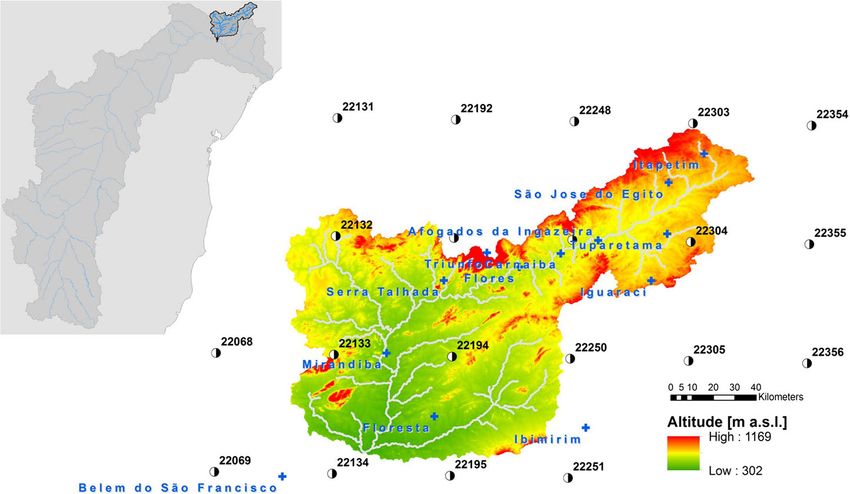
Climatic Change

to simulate the natural rainfall-runoff processes, i.e., natural river discharge. In the last step,
water management, i.e., reservoir operation and water allocation, is included to simulate
reservoir volumes and managed river discharge.

2 Data and methods

2.1 Study area

The study area is the Pajeú watershed in the Pernambuco state in north-eastern Brazil, with an
area of 16,814 km2. The watershed is part of the São Francisco river basin (Fig. 1) and drains
into the Itaparica reservoir located at the main river. The rivers in the watershed are intermit-
tent, having very low or often no flow at all during the dry season. Overall, 32 reservoirs with a
cumulative storage capacity of 595.5 million cubic meters, as well as thousands of smaller
ponds for collecting water with a cumulative estimated storage capacity of 127.0 million cubic
meters, have been constructed across the watershed (Governo do Estado de Pernambuco
1998).

2.2 Calibration and validation approaches

For the calibration and validation of the eco-hydrological model different approaches are
applied. In the first (simple) approach (A), only the observed river discharge at the most
downstream gauge is used, applying split-sample test. The second (enhanced) approach (B)
applied is according to Krysanova et al. (2018), with an enhanced 5-steps model evaluation:

i) Checking quality of observed data (river discharge) and reanalysis data/climate data used
   as climate input

Fig. 1 Overview on the Pajeú watershed with centers of WATCH cells (numbers) and meteorological observa-
tion stations (names); upper left corner, location of the Pajeú watershed within the São Francisco river basin
Climatic Change

ii) Calibration/validation to river discharges at multiple gauges (outlet and intermediate
     gauges) using a split-sample test
iii) Validation for a second variable, e.g., evapotranspiration
iv) Validation for the indicator(s) of interest
v) Validation for the observed trends or lack of trends

2.3 Set up of the SWIM model to the Pajeú watershed

The Soil and Water Integrated Model (SWIM, Krysanova et al. 2015) is a continuous-time
spatially semi-distributed eco-hydrological model. It is process-based, combining physics-
based processes and empirical approaches. It was developed from SWAT version ‘93
(Arnold et al. 1993) and MATSALU models (Krysanova et al. 1989). SWIM simulates
hydrological processes, vegetation growth, erosion, and nutrient dynamics at the river basin
scale. Hydrological response units (HRUs) considered units with same properties regarding
bio-physical processes generated by overlaying GIS-maps of land use/cover, soil, and sub-
basins are the core elements of the model. There is no lateral interaction between HRUs, but
the area-weighted HRU fluxes are added at each sub-basin outlet and routed through the river
network to the basin outlet. All processes at the HRUs level are calculated at the daily time
step. Beside spatial data, SWIM requires temporal input data, e.g., daily climate data including
precipitation, air temperature (minimum, maximum, mean), radiation, and humidity.
    SWIM has been developed for (central) European climate conditions. For the application in
the southern hemisphere, a number of adaptations were necessary (see Koch et al. 2018). For
instance, vegetation dynamics are temperature driven in (central) Europe, while they are
precipitation driven in Brazil. Also the crop rotation schemes were adjusted to two to four
harvests per year. Data on cultivated crops on municipality level from IBGE (2013) were
applied to derive crop rotations. The TURC-IVANOV approach (Wendling and Schellin
1986) was used to calculate potential evapotranspiration in the simulations.
    The reservoir module of SWIM, described in Koch et al. (2013), was applied. The reservoir
module is a conceptual representation of storage-release processes based on three management
options, to which the reservoirs are assigned: (i) objective is the minimum discharge down-
stream considering minimum and maximum reservoir volumes for each month; (ii) daily
release based on hydropower generation demand considering the minimum and maximum
reservoir volumes for each month, other restrictions can be included, e.g., daily minimum or
maximum discharges; and (iii) daily release based on the water level of the reservoir. In this
study, the operation of reservoirs is simulated applying simplistic yet realistic rules. Only
minimum and maximum reservoir volumes are considered and there is no minimum discharge
from the reservoirs. This corresponds to observational data at gauges downstream of the
reservoirs, where only during or after strong rainfall events and with reservoirs reaching
maximum volumes discharge (reservoir spill) is observed. Water is withdrawn from the
reservoirs as long as sufficient water is in the respective reservoir.
    SWIM was set up to the Pajeú watershed using soil data from De Araújo Filho et al. (2000)
and land-use data for the year 1985 from Mapbiomas (2018). The river network and 120 sub-
basins (Fig. 2) were delineated using the location of gauges and the SRTM-Digital Elevation
Model (NASA 2011). Thereafter, HRUs were derived using sub-basins, land-use, and soil
data. The nine largest reservoirs (Fig. 2 and Table 1), adding up to a storage capacity of 531.4
million cubic meters, were included in the model. Technical specifications for these reservoirs,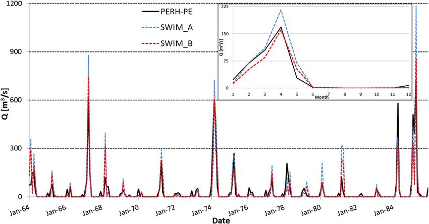
Climatic Change

Fig. 2 Sub-basins (delineated by gray lines) and sub-catchments (SC) created for Pajeú watershed, location of
gauges (red squares), and reservoirs (Açude) included in the model

e.g., water level-volume-surface area relations, were taken from APAC (2016). Observed daily
river discharge time series for six gauges from ANA (2019a) were available (Table 2). These
time series start in the 1960s or early 1970s but contain many gaps or years without any data.
Only few data on water demand/use are available. In this study, we use data from ANA
(2019b) for the reservoirs Rosário, Cachoeira II, and Serrinha II. For the other reservoirs, data
from Governo do Estado de Pernambuco (1998) are used. In all simulations including water
management, reservoir operation and water demand were held constant.

2.4 Calibration and validation: data and methods

In semi-arid regions high-rainfall intensities in combination with shallow soils and sparse
vegetation lead to a dominance of surface runoff processes in the generation of flow (Al-

Table 1 Main characteristics of largest reservoirs in the Pajeú river watershed

Name              Maximum capacity         Dead storage         Start        Sum capacity       Catchment
                  [million m3]             [million m3]         operation    [million m3]       [km2]

Saco I             36.0                     0.0                  1936         36.0              126
Arrodeio           14.5                     4.95                 1956         50.5              396
Cachoeira II       21.0                     0.03                 1965         71.6              395
Brotas             19.6                     0.02                 1978         91.2              1695
São José II         7.15                    0.11                 1981         98.3              177
Barra do Juá       71.5                     1.48                 1982        169.8              1870
Jazigo             15.5                     1.35                 1983        185.4              6170
Rosário            35.0                     1.56                 1985        220.4              1044
Serrinha II       311.0                    46.7                  1996        531.4              9948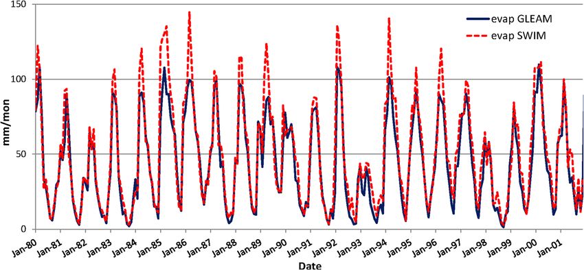
Climatic Change
Table 2 Observational gauges in the Pajeú river watershed
Gauge Catchment [km2] Altitude [masl] Start operation
Afogados da Ingazeira 3539 540 1964
Flores 4965 464 1967
Serra Talhada 5912 424 1972
Serrinha 9639 376 1964
Floresta 12,266 318 1972
Ilha Grande 2273 379 1964
Weshah 2002). Due to the dominance of surface runoff processes sampling errors in rainfall
data, e.g., due to a low density rainfall gauge network, can have significant effects in rainfall-
runoff simulations (Pilgrim et al. 1988; Michaud and Sorooshian 1994). Small deviations in
rainfall data can lead to strong differences between observed and simulated flows and the
usefulness of using performance indicators like Nash-Sutcliffe efficiency (NSE—Nash and
Sutcliffe 1970) in semi-arid regions has been questioned, e.g., by Costelloe et al. (2005). For
instance, Love et al. (2011) achieved a NSE value higher 0.3 for only one out of 13 catchments
in the Limpopo river basin. According to Moriasi et al. (2007), NSE values lower than 0.5
should be rated as “unsatisfactory”, a rating that may be appropriate for perennial rivers. For
intermittent rivers, it seems more appropriate to use graphical analysis and long-term daily
mean river discharge (cf. Figs. 3 and 4), because then single under- or overestimations in
rainfall are leveled out to a certain degree while capturing the annual cycle.
The calibration and validation was done manually using mainly graphical analysis as proposed
by Legates and McCabe (1999). This manual calibration also helped in understanding the hydro-
meteorological characteristics and processes of the region. To determine the parameter sets also
annual mean river discharges (cf. Fig. S9 in the Supplementary Material) and the goodness of fit
using the NSE were applied. An NSE equal to 1 represents a perfect fit. Furthermore, bias, percent
bias (PBIAS), and root mean squared error (RMSE) were applied as criteria.
The data in Table 1 indicate that over time the storage volume in reservoirs has increased
significantly. To exclude the effects of water management on river discharge, it is advisable to
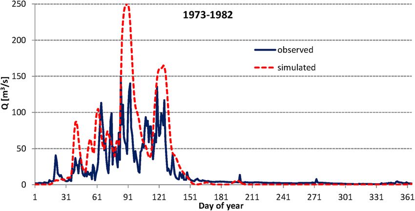
Fig. 3 Comparison of long-term mean daily discharge at gauge Floresta (1973–1982) observed and simulated
with SWIM_A after calibration using the simple approach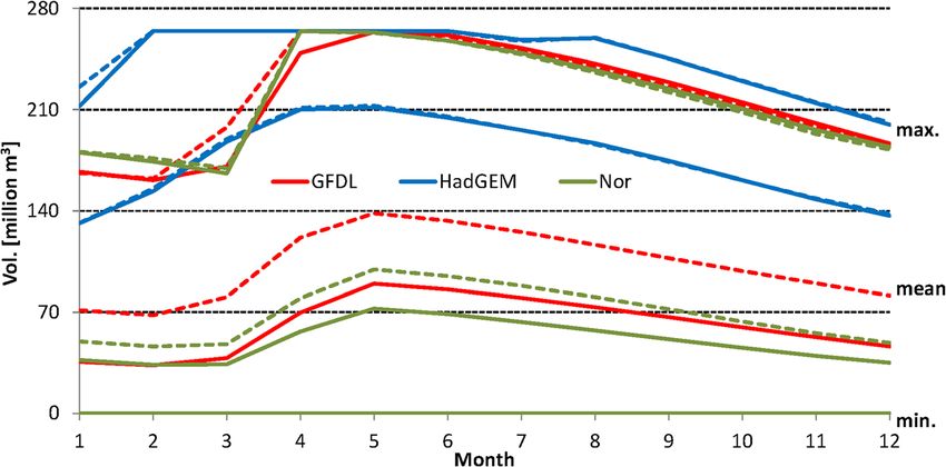
Climatic Change

Fig. 4 Comparison of long-term mean daily discharge at gauge Floresta (1973–1982) observed and simulated
with SWIM_B after calibration using the enhanced approach

use observed discharges from the 1960s or 1970s for the calibration and validation. Table 2
shows that the observational time series for some gauges only start in the 1970s. This, and
many gaps in the observational time series, restricts the use of the same time period for the
calibration and validation at different gauges. Therefore, for different gauges, different time
periods for the calibration and validation were used. Two gridded global climate data sets were
analyzed, WATCH Forcing Data (Weedon et al. 2011) based on ERA-40 reanalysis and
meteorological observations (Uppala et al. 2005) for the years 1960 to 2001, in the following
“WATCH-ERA40”, and WATCH Forcing Data based on ERA-Interim reanalysis and mete-
orological observations (Weedon et al. 2014) for the years 1979 to 2010, in the following
“WATCH-INTERIM”. As daily climate data from the 1960s and 1970s are needed to calibrate
the SWIM model to observed river discharges with low water management impact the
WATCH-ERA40 data set is used.
   Beside observed river discharge data for the gauges in Table 2 further data were used to
validate the model in the second approach following Krysanova et al. (2018). Monthly actual
evapotranspiration sums of SWIM for the years 1980 to 2001 are compared to results of
GLEAM (Martens et al. 2017). For the calibration of SWIM, time periods in the 1960s and
1970s were used. Therefore, this comparison was not used for the calibration but for validating
the model. Beside the simulated time series averaged over the watershed also the long-term
annual spatial distributions are compared.
   In the Federal Water Resources Plan of Pernambuco (Governo do Estado de Pernambuco
1998), simulation results for the Pajeú watershed from the model GRH (Grupo de Recursos
Hídricos, developed at the Federal University of Pernambuco, based on the model SMAP—
Lopes et al. 1982) with monthly time step are available for the time period 1964 to 1985. These
results are also used to validate the model.

2.5 Checking of global gridded climate data

Before starting the calibration of SWIM the climate input was analyzed. Observed meteorological
data from INPE (Instituto Nacional de Pesquisas Espaciais) for the years 1964 to 2015 and two
Climatic Change

gridded global data sets (WATCH-ERA40 and WATCH-INTERIM) were applied. Figure S1
(Supplementary Material) shows that WATCH-INTERIM data, starting in 1979, have signifi-
cantly higher annual precipitation sums than the data of INPE and WATCH-ERA40. From Fig.
S1 can also be derived that until 1987 annual precipitation sums of INPE and WATCH-ERA40
are very similar but after 1987 start to deviate, with WATCH-ERA40 showing visibly higher
values. On the monthly time-scale, differences between INPE and WATCH-ERA40 data can be
found also before 1988. For instance, annual precipitation sums are very similar in the years 1970
and 1971 but can reach differences up to 40 mm/month (Fig. S2). Also, the intensity of
precipitation events in both data sets differs (Fig. S3). The data of INPE contain more days per
year with low to medium intensity precipitation events (defined as days with precipitation of 2–
20 mm/day), the WATCH-ERA40 data contain a higher number of days per year with high
intensity precipitation events (precipitation > 20 mm/day). Due to its hydro-climatic characteris-
tics the watershed has a very fast response to precipitation. To illustrate this, results using SWIM
calibrated according to the enhanced approach driven by data of INPE and WATCH-ERA40 are
shown in Fig. S4.
    Because of the overestimation of high intensity precipitation events in the WATCH-
ERA40 data set, a bias correction based on quantile mapping was carried out. For the 30-
year period 1972 to 2001, quantile values of WATCH-ERA40 were adjusted to corre-
sponding quantile values of observations. Percentiles of daily precipitation were calcu-
lated for different regions, selected according to the gauges, e.g., region upstream of
Flores, region between Flores and Serra Talhada. The transfer functions for the different
regions were derived from daily observed and WATCH-ERA40 precipitation values, see
Fig. S5. The strongest correction was necessary in the north-eastern part of the water-
shed, i.e., the region upstream of gauge Flores. Due to the low density of meteorological
stations no correction was carried out in the south-eastern part of the watershed (gauge
Ilha Grande, see Fig. 1).
    Because the aim of the study was to analyze the effects of two different calibration
approaches, the corrected precipitation data were used in approaches A and B.

3 Results

3.1 Calibration and validation approach A

Results are given on daily or monthly time steps, trying to keep the most important features of
simulated river discharges and reservoir volumes.
   In the first approach, the model (SWIM_A) is calibrated, applying the WATCH-ERA40
data set, to the most downstream gauge (Floresta), covering an area of 12,266 km2 of the
overall 16,814 km2. Gauge Ilha Grande (see Fig. 1) is located at the tributary Riacho Do
Návio which flows into the Pajeú main river downstream of gauge Floresta. During the
calibration and validation, graphical comparison of daily (Fig. S6) and the long-term mean
daily flows at gauge Floresta (Fig. 3) was applied. In Table 3 annual flows and criteria for the
calibration and validation periods are given. The most sensitive parameters in the calibration
were ecal (correction factor for potential evaporation), roc parameters (routing coefficients
to calculate the storage time constant), sccor (correction factor for saturated conductivity),
bff (baseflow factor), delay (groundwater delay), and abf (groundwater recession). The
parameters determined are given in Table S1.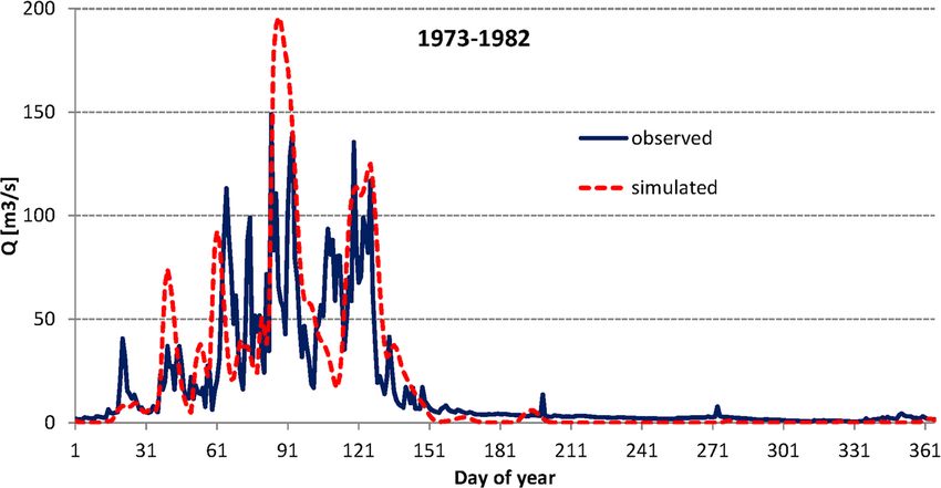
Climatic Change

Table 3 Results for calibration (1973–1977) and validation (1978–1982) at gauge Floresta, SWIM_A and SWIM_B

Year             1973           1974     1975        1976        1977       1978         1979      1980       1981     1982      Mean      Mean

Q obs. [m3/s]        8.27       53.7      33.8          4.97     14.2       16.8         7.45      8.08       28.2        5.18   23.0      13.2     SWIM_A
Q sim. [m3/s]        5.26       106.8     45.5          3.49     21.5       19.1         15.2      16.5       34.5        0.56   36.5      17.2
BIAS [m3/s]        − 2.26       37.2      17.8        − 1.09       7.67       2.24       8.75      15.0       13.6      − 4.37   11.9      7.04
PBIAS [%]         − 27.3        69.2      52.7       − 22.0      54.1       54.1         117       185        48.2     − 84.4    25.3      64.1
RMSE [m3/s]         22.8        214.2    103.6         20.6      56.0       59.9         55.9      79.0       93.2       12.6    83.4      60.1
NSE (daily)          0.29       − 2.18   − 0.62       − 0.04     − 1.40     − 0.36       − 10.4    − 9.97       0.29    − 0.01   − 0.79    − 4.10
NSE (mon)            0.73       0.03       0.65         0.62     − 1.74       0.12       − 6.10    − 12.0       0.52    − 0.22   0.06      − 3.54
Q obs. [m3/s]        8.27       53.7      33.8          4.97     14.2       16.8         7.45      8.08       28.2        5.18   23.0      13.2     SWIM_B
Q sim. [m3/s]        4.29       79.7      29.6          2.89     15.5       12.7         9.90      8.74       23.0        0.63   26.4      11.0
BIAS [m3/s]        − 3.40       12.4       1.37       − 1.06       1.54     − 4.16       3.12      4.03       − 0.28    − 4.30   2.16      − 0.32
PBIAS [%]         − 41.1        23.0       4.05      − 21.2      10.9       10.9         41.8      49.9       − 0.98   − 82.9    − 4.87    3.74
RMSE [m3/s]         21.1        185       69.4         18.9      40.9       50.4         37.2      41.8       79.5       12.4    67.1      44.3
NSE (daily)          0.39       − 1.37     0.27         0.13     − 0.28       0.04       − 4.07    − 2.08       0.49      0.02   − 0.17    − 1.12
NSE (mon)            0.81       0.65       0.99         0.55     − 0.04       0.29       − 1.52    − 0.93       0.98    − 0.19   0.59      − 0.27
                  Calibration                                               Validation                                           Calibr.   Valid.
Climatic Change
Although the general characteristics of the runoff regime can be reproduced, high flows are
often overestimated (Fig. S6 and Fig. 3) and therefore the mean annual flows are also
overestimated (Table 3). Any attempt to reduce simulated high flows, e.g., in 1974 or 1975,
would lead to an even stronger underestimation of river discharges in rather dry years, e.g.,
1973 or 1976.
3.2 Calibration and validation approach B
In this approach, the model is calibrated to six gauges (Table 2) from upstream to downstream. For
calibration and validation, four sub-catchments (conglomerates of SWIM sub-basins, see Fig. 2)
were defined and for each sub-catchment a specific parameter set was derived. The application of
different parameter settings for each sub-catchment enabled a better adjustment of the model to local
conditions, e.g., soil and land-use properties or topography. For instance, the northern and north-
eastern part of the catchment is characterized by mountains, while the south is characterized by
lowlands. When creating the four sub-catchments not only the location of gauges but also other
factors, e.g., topographic gradient, were taken into consideration and therefore borders of sub-
catchments do not necessarily coincide with locations of gauges.
Results for gauge Flores as an example for an intermediate gauge are displayed in Fig. S7.
Figure S8 and Fig. 4 show results for gauge Floresta and Table 3 gives criteria for the
calibration and validation periods. The parameter settings determined for the four sub-
catchments are given in Table S1.
In Fig. S9, the annual mean flows at gauge Floresta observed and simulated applying
SWIM_A and SWIM_B are displayed. In general, except for very dry years, the river
discharges simulated by SWIM_A are higher than simulations of SWIM_B and observations.
Overall, SWIM_B shows a better performance than SWIM_A.
As a second variable (step 3) for the validation of SWIM_B actual evapotranspiration (years
1980 to 2001) is compared to results of the model GLEAM (Martens et al. 2017). Monthly actual
evapotranspiration sums (Fig. 5) give somewhat higher values for SWIM_B in the rainy season. As
actual evapotranspiration depends on potential evaporation but also on water availability and hence
on precipitation, the different sources for precipitation data can explain these differences. In Fig. S10
Fig. 5 Comparison of monthly actual evapotranspiration sums from models GLEAM and SWIM_B after
calibration using the enhanced approachClimatic Change
monthly and annual actual evapotranspiration sums are displayed. The spatial distributions of actual
evapotranspiration are shown in Fig. S11. Overall, the results of GLEAM and SWIM_B show
comparable annual cycles, monthly and annual sums, and spatial distributions.
Simulated river discharge data for the outlet of the Pajeú river, i.e., the inflow into the São
Francisco river, from Governo do Estado de Pernambuco (1998), here named PERH-PE, are
utilized for further validation of SWIM. Time series of mean monthly data for the time period
1964 to 1985 are compared in Fig. 6. The results of SWIM_B are much closer to the data of
PERH-PE than those of SWIM_A.
Step 5, i.e., validation for observed trends or lack of trends, of the approach presented by
Krysanova et al. (2018) is not carried out, because the number and the storage capacity of
reservoirs have increased significantly over the last decades (see Table 1) and any trend caused
by hydro-climatological changes in the observed river discharge time series is obscured by
human activities.
3.3 Water management simulations
In the next step, water resources management is included in the simulations. Irregular daily
measurements of water levels and volumes for a number of reservoirs are available (APAC
2017). Most of these data cover only the last few years and for the time period until 2001 only
data for two reservoirs included in SWIM are available.
The reservoirs in the Pajeú watershed are operated in a very simplistic way: water is stored
up to full volume, further volumes are spilled uncontrolled. Minimum/ecological discharge
requirements are not considered, but the entire stored water is used for water supply, mainly
potable and irrigation water. This is shown in Fig. S13, where observed and simulated
discharges at gauge Serrinha II downstream of reservoir Serrinha II are displayed (years
1998 to 2001 without discharge). In all simulations including water management reservoir
operation is not changed in order to only assess the effects and uncertainties resulting from the
two different calibration approaches and the climate scenarios.
Fig. 6 Time series of simulated monthly discharge at the outlet of the Pajeú river according to PERH-PE
(Governo do Estado de Pernambuco 1998), with SWIM_A (simple approach) and with SWIM_B (enhanced
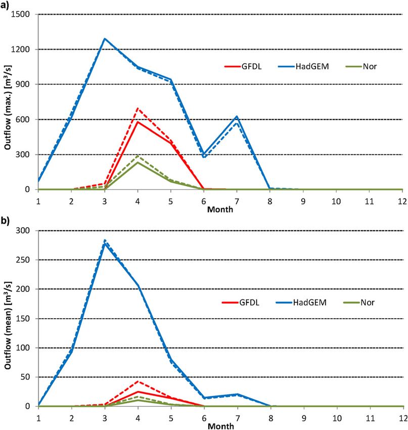
approach); inlet, simulated long-term mean monthly dischargesClimatic Change In Fig. S12 observed and simulated volumes for the reservoirs Rosario and Brotas are displayed. For reservoir Rosario, in normal to wet years from 1994 to 1997, the differences between the results of SWIM_A and SWIM_B are low, but volumes are much higher than observed ones. The very dry year 1998 is visible in the simulated and the observed volumes. The reliability of observed volumes cannot be assessed, but some values seem to be unreliable, e.g., certain values in the year 2000. For reservoir Brotas in the normal to wet years from 1994 to 1997 volumes simulated by SWIM_A, SWIM_B, and observed volumes are similar. The very dry year 1998 is visible in the simulated and the observed volumes. From 1999 onward, there are differences between observed and simulated volumes, but also differences between simulations are larger than before 1998. The operation of reservoir Serrinha II started in 1996. Only in wet years, with the reservoir reaching its maximum volume, discharge is observed (Fig. S13). In the simulations, spill is occurring more often, especially in simulations by SWIM_A. 3.4 Earth system model data and simulations for the reference period Applying a trend-preserving method, WATCH-ERA40 data were used by Hempel et al. (2013) to regionalize and bias-correct the five ESMs HadGEM2-ES, IPSL-CM5A-LR, Fig. 7 Changes in natural discharge ((2021/2050)–(1976/2005)) simulated with SWIM_A (dashed lines) and SWIM_B (continuous lines). Maximum mean monthly a RCP2.6 and b RCP8.5. Long-term mean monthly c RCP2.6 and d RCP8.5. Change averaged over all five ESM e RCP2.6 and f RCP8.5
Climatic Change

MIROC-ESM-CHEM, GFDL-ESM 2M, and NorESM1-M in the framework of ISIMIP
(Warszawski et al. 2014). The SWIM model with two different parameter sets (SWIM_A
and SWIM_B) was applied to simulate reference and future periods forced by the ESMs. A
detailed analysis of SWIM simulations using ESM data for the reference period is given in the
Supplementary Material (the section “Earth system model data and simulations for the
reference period”), where Figs. S14 to S20 show results for natural discharges and simulations
including water management.

3.5 Climate change impact simulations for natural river discharge

For analyzing simulated climate change impacts, with parameter settings according to the
simple (SWIM_A) and enhanced approach (SWIM_B), results for the near future, i.e., period
from 2021 to 2050, are used.
   Figures 7a and b illustrate the change in natural maximum mean monthly river discharges at
gauge Floresta for all five ESM for RCP2.6 and RCP8.5, respectively. For IPSL a clear increase
of maximum discharges in the main rainy season (here defined as February to May) is simulated
for both RCPs and the SWIM model with both parameter sets, except for April under RCP8.5
(Table S3). Simulations using GFDL, MIROC, and HadGEM do not show a clear signal, i.e.,
there are months with increase and months with decrease in maximum discharges. In simula-
tions using Nor, a decrease in maximum discharges is found, except for March under RCP8.5
using SWIM_A with a small increase of 3.2%. The differences in changes between SWIM_A
and SWIM_B averaged over all ESMs are below 5% for the months March and April.
   Figures 7c and d show the change in long-term mean monthly discharges at gauge Floresta
for RCP2.6 and RCP8.5, respectively. For RCP2.6 using IPSL and HadGEM, a clear increase
in mean discharge is simulated, while simulations based on the other three ESMs show a clear
decline. Under RCP8.5, all ESM simulations, except IPSL, lead to a decrease in mean
discharges. Differences between long-term mean monthly discharges based on SWIM_A and
SWIM_B averaged over all ESMs for the same RCP are low in general. Larger differences are
found when comparing RCP2.6 and RCP8.5. The differences in changes between SWIM_A
and SWIM_B averaged over all ESMs are 8% under RCP2.6 and 2% under RCP8.5 (Table S4).
   Figures 7e and f show the averaged change simulated for maximum and long-term mean
monthly discharges for all ESMs. Overall, under RCP2.6 an increase of mean discharge is
simulated for the first part of the rainy season and a small decrease at the end of the rainy season,
while under RCP8.5 the trend is negative. For maximum discharges there is no clear trend, i.e.,
there are months with a strong decrease while other months show a clear increase. The strong
decline in maximum discharge for the month of July under RCP8.5 is caused by simulations
using HadGEM that show a peak in July in the reference period (see Figs. S15 and S17). This
peak in July is also found under RCP2.6 using HadGEM in the future period 2021 to 2050.
   Changes in minimum mean monthly discharges are not shown as they are zero in almost all
months.

3.6 Climate change impact simulations including water management

Results for the simulations including water management are presented for reservoir Serrinha II
because it is the largest reservoir and includes the effects of all other reservoirs except reservoir
Barra do Juá. Only results using HadGEM, GFDL, and Nor are presented to reduce the
complexity of the graphs. HadGEM represents a wet simulation, GFDL a medium, and Nor a
Climatic Change

Fig. 8 Simulated minimum, long-term, and maximum mean monthly volumes of reservoir Serrinha II, simulated
with SWIM_A (dashed lines) and SWIM_B (continuous lines) for RCP2.6 (years 2021–2050) for ESM
HadGEM, GFDL and Nor

dry simulation. Results for minimum, long-term, and maximum mean monthly volumes of
reservoir Serrinha II under RCP2.6 are shown in Fig. 8. Minimum volumes are zero in all
simulations, while mean volumes are highest using HadGEM and lowest using Nor. The
simulated mean volumes using GFDL and Nor are higher when applying SWIM_A, on
average higher by 41.8 million cubic meters or 74% (GFDL) and 19.4 million cubic meters
or 39% (Nor). Such differences are not found for HadGEM. Maximum volumes are highest
using HadGEM, while the results using GFDL and Nor are comparable.
    Minimum mean monthly volumes for reservoir Serrinha II are zero in all simulations under RCP8.5
(Fig. S21). Simulated mean volumes are highest using HadGEM and lowest using Nor. The highest
mean volumes using Nor and GFDL are simulated with SWIM_A. This differentiation between
SWIM_A and SWIM_B is much less pronounced for HadGEM. Maximum volumes are highest
using HadGEM and somewhat lower using GFDL. Nor gives the lowest maximum volumes.
    Simulated maximum and long-term mean monthly discharges of reservoir Serrinha II for
RCP2.6 are shown in Fig. 9a and b, respectively. Water is only discharged when the reservoir
reaches its maximum capacity. Discharges are highest using HadGEM and lowest using Nor.
Higher discharges are simulated using SWIM_A and generally lower using SWIM_B. In the
month of April, the simulated discharges using GFDL and Nor are higher applying SWIM_A.
Maximum and long-term mean monthly discharges are 20% and 69% higher using GFDL, 24%
and 69% higher using Nor, respectively. Comparable results are found for RCP8.5 (Fig. S22).
    The differences between changes in maximum mean monthly volume of reservoir Serrinha II
with SWIM_A and SWIM_B (Table S5) can reach 10% under RCP2.6 (GFDL in March) and 29%
under RCP8.5 (GFDL in February). Averaged over all ESMs differences between SWIM_A and
SWIM_B are up to 9.2% under RCP2.6 (April) and 10.2% under RCP8.6 (December).
    The differences between changes in long-term mean monthly volume of reservoir Serrinha
II with SWIM_A and SWIM_B (Table S6) can reach 20% under RCP2.6 (GFDL in March)
and 21% under RCP8.5 (IPSL in February). Averaged over all ESMs differences between
SWIM_A and SWIM_B are below 5% under both RCP.
    The change in maximum mean monthly reservoir inflow averaged over all ESMs using SWIM_A
is − 23% (March) and − 13% (April) under RCP2.6 and using SWIM_B − 21% (March) and − 18%
Climatic Change
Fig. 9 Simulated a maximum mean monthly and b long-term mean monthly discharge of reservoir Serrinha II,
simulated with SWIM_A (dashed lines) and SWIM_B (continuous lines) for RCP2.6 (years 2021–2050)
(April); under RCP8.5 using SWIM_A the change is − 9.3% (March) and + 2.5% (April) and using
SWIM_B − 6.2% (March) and + 1.4% (April). Averaged over all ESMs notable differences in
changes (5%) between SWIM_A and SWIM_B are found under RCP2.6 in April.
The change in maximum mean monthly reservoir discharge averaged over all ESMs using
SWIM_A is − 22% (March) and − 13% (April) under RCP2.6 and using SWIM_B − 21% (March)
and − 20% (April); under RCP8.5 using SWIM_A the change is − 5.5% (March) and + 0.9% (April)
and using SWIM_B − 2.7% (March) and − 1.0% (April) (Table S7). Averaged over all ESMs notable
differences in changes (6.5%) between SWIM_A and SWIM_B are found under RCP2.6 in April.
The differences in changes in long-term mean reservoir inflow between SWIM_A and
SWIM_B averaged over all ESMs are 7.5% under RCP2.6 and 2% under RCP8.5 (Table S8).
The differences in changes in long-term mean reservoir discharge between SWIM_A and
SWIM_B averaged over all ESMs are 10% under RCP2.6 and 2% under RCP8.5 (Table S8).
4 Discussion and conclusions
Two approaches to calibrate and validate an eco-hydrological model were applied. In the simple
approach (SWIM_A), only the lowermost gauge was used. In the enhanced approach (SWIM_B),
the model was calibrated also to river discharge at intermediate gauges and furthermore validatedClimatic Change
using actual evapotranspiration. The enhanced approach is much more time consuming but
increases the reliability of the simulations, e.g., by using a second, spatial variable for validation
(here evapotranspiration). The concept described by Krysanova et al. (2018) is a step forward, e.g.,
checking quality of used weather and discharge data, calibration not only at outlet and using a
second variable. But the approach is rather inflexible and difficult to apply in river basins where
water management has a strong effect on river discharge and should be further developed accord-
ingly. Maybe some lesson learned from this study could be that when selecting intermediate gauges,
the location of large lakes and reservoirs/water infrastructure should be taken into account, i.e.,
gauges should be located upstream of these. Overall, an analysis of effects of water management/
reservoir operation on river discharges should be made before using discharges for calibrating
hydrological models or before carrying out a trend analysis.
The differences in changes in natural mean discharge for the time period 2021 to 2050 compared
to the reference period (1976 to 2005) between SWIM_A and SWIM_B averaged over all five ESM
are notable (8%) under RCP2.6 but negligible (2%) under RCP8.5. The different calibration
approaches show the highest differences in simulated maximum mean monthly discharges and
the changes can even show different directions. The reason for these differences can be explained by
the two different parameter sets. While the correction factor for evapotranspiration may not affect
simulations of maximum discharges distinctly, the groundwater parameter values have a strong
effect on simulated mean and maximum discharges. To reduce high river discharges in SWIM_A
parameter values are set to slow down the system reaction to precipitation input. The time until
precipitation becomes runoff is prolonged. This also can be seen when comparing Figs. 3 and 4,
where the falling limb after high flows is longer in simulations with SWIM_A. Applying parameter
values that simulate a faster response of the system would increase simulated river discharges that
are already much higher than observed ones in normal and wet years (see Figs. S6 and S9). Overall,
the model calibrated applying the enhanced approach (SWIM_B) better represents the hydrological
processes in the different parts of the watershed and therefore is considered more robust.
Furthermore, it is important to mention that the hydrological processes are calibrated in both
approaches to observed river discharges before 1983, with low effects of water management, and
applying bias-corrected WATCH-ERA40 precipitation data. Under the assumption that the simple
approach does not consider quality checking of observational data, e.g., river discharge or climate input,
and other information, e.g., reservoirs upstream of a gauge, data from 1983 onward with huge impacts
of reservoirs on observed river discharge could have been used for the calibration. With the number and
capacity of reservoirs increasing, lower river discharge is observed downstream of reservoirs. Directly
downstream of reservoirs discharge is only observed during or after high intensity precipitation events.
Model calibration based on observed river discharges after 1983 with strong water management impacts
would have resulted in a different parametrization applying the simple approach.
Especially in data scarce or semi-arid regions where precipitation input for hydrological
simulations contains huge uncertainties, the use of more than one variable, e.g., evapotranspi-
ration in addition to observed river discharge, is recommended for further validation of
hydrological models.
Because of the very fast reaction of the hydrological system in semi-arid regions differences in
the precipitation input can cause huge differences in simulated river discharges and the use of
performance indicators like Nash-Sutcliffe efficiency (NSE) has been questioned. For rivers with
high contribution of baseflow, i.e., buffering of precipitation input and slow decline of discharge
after precipitation events, the differences of NSE for daily and monthly time steps are usually low. In
regions with high fluctuations in runoff, using NSE with daily or monthly simulation time step as
performance indicator is questionable. Applying SWIM_B at daily or monthly time step can giveClimatic Change
contradictory results, e.g., NSE is below 0.5 (unsatisfactory) for the years 1975 and 1981 with daily
time step, and NSE of 0.99 and 0.98 (perfect) for the same years with monthly time step.
For the reference period, simulations using data of one ESM (HadGEM) give much higher
maximum and long-term mean monthly river discharges compared to observations and other
simulations. In the simulations for the future, period one ESM (IPSL) gives higher maximum and
long-term mean monthly discharges for almost all months in the main rainy season compared to
simulations under reference conditions under both RCPs. Using data of Nor lower maximum and
long-term mean, monthly discharges are simulated under both RCPs compared to simulations under
reference conditions. For the other three ESMs (HadGEM, MIROC, GFDL) there is no clear overall
trend, while the change signal in some months is very clear. In general the model calibrated applying
the simple approach (SWIM_A) simulates stronger change signals than the model calibrated
applying the enhanced approach (SWIM_B).
The higher river discharges simulated by SWIM_A translate to higher reservoir volumes
and uncontrolled discharges (spill) in simulations including water management. The differ-
ences in changes in mean discharge from reservoir Serrinha II for the future period compared
to the reference period between SWIM_A and SWIM_B averaged over all ESMs are notable
(10%) under RCP2.6 but negligible (2%) under RCP8.5.
Overall, differences in changes in natural and managed mean discharges are negligible
under RCP8.5 but notable under RCP2.6 for the ESM ensemble mean, i.e., the differences in
changes depend on the model calibration and validation approach but also on the RCP.
The differences between changes in maximum mean monthly volumes of reservoir Serrinha II
averaged over all ESMs are notable in some months under both RCPs, while difference are negligible
for long-term mean monthly volumes. Differences between changes in maximum mean monthly
reservoir inflows and reservoir discharges averaged over all ESMs are notable under RCP2.6 in April.
In this study, a simplistic reservoir operation, focusing on local water supply, is applied. In
another paper of Koch et al. (2018), where SWIM is applied to the entire São Francisco river
basin with huge reservoirs operated for hydropower generation, water supply, flood control, and
maintaining minimum discharges downstream of reservoirs, a much more elaborated reservoir
operation is simulated. Due to low data availability for observed reservoir volumes and water
demand/use, the results in the present study including water management should be considered
a first approximation. The water management simulations mainly serve the purpose to demon-
strate the differences between natural and managed river discharges. Furthermore, the objective
was to analyze the impacts of applying two different parameter sets in the eco-hydrological
model and data of different ESMs and RCPs in the water management simulations.
This study also shows the necessity to include a number of different ESMs and RCPs in
climate impact studies on hydrological processes and water management.
Supplementary Information The online version contains supplementary material available at https://doi.
org/10.1007/s10584-020-02917-w.
Funding Open Access funding enabled and organized by Projekt DEAL. This work has been conducted within
the bi-national (Brazil and Germany) research project INNOVATE funded by the German Ministry of Education
and Research (BMBF, grant numbers 01LL0904 A and D) and the Brazilian Council of Scientific and
Technologic Development (CNPq), Ministry of Science, Technology e Innovation (MCTI) and Federal Univer-
sity of Pernambuco (UFPE), and under the framework of ISI-MIP2b. The ISI-MIP2b project was funded by the
German Federal Ministry of Education and Research (BMBF) with project funding reference number
01LS1201A2.
Responsibility for the content of this publication lies with the authors.Climatic Change
Open Access This article is licensed under a Creative Commons Attribution 4.0 International License, which
permits use, sharing, adaptation, distribution and reproduction in any medium or format, as long as you give
appropriate credit to the original author(s) and the source, provide a link to the Creative Commons licence, and
indicate if changes were made. The images or other third party material in this article are included in the article's
Creative Commons licence, unless indicated otherwise in a credit line to the material. If material is not included
in the article's Creative Commons licence and your intended use is not permitted by statutory regulation or
exceeds the permitted use, you will need to obtain permission directly from the copyright holder. To view a copy
of this licence, visit http://creativecommons.org/licenses/by/4.0/.
References
Al-Weshah RA (2002) Rainfall-runoff analysis and modelling in wadi systems. In: H Wheater, RA Al-Weshah
(eds.): Hydrology of wadi systems. INTERNATIONAL HYDROLOGICAL PROGRAMME, technical
documents in hydrology no. 55, UNESCO, Paris, 159 p., 87-112
ANA (2019a) Sistema Nacional de Informações sobre Recursos Hídricos (National system for information on
water resources). Agência Nacional de Águas (Brazilian National Water Agency). http://www.snirh.gov.
br/hidroweb/serieshistoricas (last accessed: 14-11-2019)
ANA (2019b) Outorgas Emitidas pela ANA (Water rights emitted by ANA). Agência Nacional de Águas
(Brazilian National Water Agency). http://portal1.snirh.gov.br/ana/apps/webappviewer/index.html?id=0d9
d29ec24cc49df89965f05fc5b96b9 (last accessed: 26-11-2019)
APAC (2016) Fichas técnicas (Technical data sheets). Agencia Pernambucana de Águas e Clima (Pernambuco
water and climate agency). http://200.238.109.99:8080/apacv5/fichareservatorio_web/fichareservatorio_
web.php; (last accessed: 19.09.2016)
APAC (2017) Histórico (Historical). Agencia Pernambucana de Águas e Clima (Pernambuco water and climate
agency). http://200.238.109.99:8080/apacv5/cons_monitora_web/cons_monitora_web.php; (last accessed:
19.01.2017)
Araújo JC, Bronstert A (2016) A method to assess hydrological drought in semi-arid environments and its
application to the Jaguaribe River basin, Brazil. Water Int 41:213–230. https://doi.org/10.1080
/02508060.2015.1113077
Arnold JG, Allen PM, Bernhardt G (1993) A comprehensive surface groundwater flow model. J Hydrol 142:47–
69
Balme M, Vischel T, Lebel T, Peugeot C, Galle S (2006) Assessing the water balance in the Sahel: impact of
small scale rainfall variability on runoff, part 1: rainfall variability analysis. J Hydrol 331:336–348
Bracken LJ, Cox NJ, Shannon J (2008) The relationship between rainfall inputs and flood generation in south-
east Spain. Hydrol Process 22:683–696
Callow JN, Smettem KRJ (2009) The effect of farm dams and constructed banks on hydrologic connectivity and
runoff estimation in agricultural landscapes. Environ Model Softw 24:959–968. https://doi.org/10.1016/j.
envsoft.2009.02.003
Camarasa AM, Tilford KA (2002) Rainfall-runoff modelling of ephemeral streams in the Valencia region
(eastern Spain). Hydrol Process 16:3329–3344
Costelloe JF, Grayson RB, McMahon TA (2005) Modelling stream flow for use in ecological studies in a large,
arid zone river, Central Australia. Hydrol Process 19:1165–1183
De Araújo Filho JC et al. (2000) Levantamento de reconhecimento de baixa e média intensidade dos solos do
Estado de Pernambuco. Embrapa Solos (Boletim de pesquisa 11), Rio de Janeiro. 378p
Gädeke A, Hölzel H, Koch H, Pohle I, Grünewald U (2014) Analysis of uncertainties in the hydrological
response of a model-based climate change impact assessment in a subcatchment of the Spree River,
Germany. Hydrol Process 28:3978–3998
Governo do Estado de Pernambuco (1998) Plano Estadual de Recursos Hídricos de Pernambuco - PERH-PE
(Federal water resources plan of Pernambuco). Vol. 2, Parte IV - Recursos Hídricos Superficiais. Recife:
Secretaria de Recursos Hídricos. 218p
Hempel S, Frieler K, Warszawski L, Schewe J, Piontek F (2013) A trend-preserving bias correction — The ISI-
MIP approach. Earth Syst Dynam Discuss 4:49–92
IBGE (2013) Produção agrícola municipal (Agricultural production on municipality level). Instituto Brasileiro de
Geografia e Estatística (Brazilian Institute of Geography and Statistics). https://seriesestatisticas.ibge.gov.
br/lista_tema.aspx?op=0&de=83&no=1. Accessed 13 Dec 2013
Koch H, Liersch S, Hattermann FF (2013) Integrating water resources management in eco-hydrological
modelling. Water Sci Technol 67:1525–1533Climatic Change
Koch H, Liersch S, de Azevedo JRG, Silva ALC, Hattermann FF (2018) Assessment of observed and simulated
low flow indices for a highly managed river basin. Hydrol Res (online). https://doi.org/10.2166/nh.2018.168
Krysanova V, Meiner A, Roosaare J, Vasilyev A (1989) Simulation modelling of the coastal waters pollution
from agricultural watershed. Ecol Model 49:7–29
Krysanova V, Hattermann F, Huang S, Hesse C, Vetter T, Liersch S, Koch H, Kundzewicz ZW (2015)
Modelling climate and land-use change impacts with SWIM: lessons learnt from multiple applications.
Hydrol Sci J 60:606–635
Krysanova V, Donnelly C, Gelfan A, Gerten D, Arheimer B, Hattermann F, Kundzewicz ZW (2018) How the
performance of hydrological models relates to credibility of projections under climate change. Hydrol Sci J
63:696–720
Legates DR, McCabe GJ Jr (1999) Evaluating the use of "goodness-of-fit" measures in hydrologic and
hydroclimatic model validation. Water Resour Res 35:233–241
Liersch S, Tecklenburg J, Rust H, Dobler A, Fischer M, Kruschke T, Koch H, Hattermann FF (2018) Are we
using the right fuel to drive hydrological models? A climate impact study in the Upper Blue Nile. Hydrol
Hydrol Earth Syst Sci 22:2163–2185
Lopes JEG, Braga BPF Jr, Conejo JGL (1982) SMAP - a simplified hydrological model, applied modelling in
catchment hydrology. In: Singh VP (ed) Water resources publication. Littleton, Colorado, USA, pp 167–176
Love D, Uhlenbrook S, van der Zaag P (2011) Regionalising a meso-catchment scale conceptual model for river
basin management in the semi-arid environment. Phys Chem Earth, Parts A/B/C 36:747–760. https://doi.
org/10.1016/j.pce.2011.07.005
Malveira V, Araújo J, Güntner A (2012) Hydrological impact of a high-density reservoir network in semiarid
northeastern Brazil. J Hydrol Eng 17:109–117. https://doi.org/10.1061/(ASCE)HE.1943-5584.0000404
MAPBIOMAS (2018) Project MapBiomas - collection 2.3 of Brazilian land cover & use map series, accessed on
06-09-2018 through the link: http://mapbiomas.org
Martens B et al (2017) GLEAM v3: satellite-based land evaporation and root-zone soil moisture. Geosci Model
Dev 10:1903–1925
Michaud JD, Sorooshian S (1994) Effect of rainfall-sampling errors on simulations of desert flash floods. Water
Resour Res 30:2765–2775
Moriasi DN, Arnold JG, Van Liew MW, Bingner RL, Harmel RD, Veith TL (2007) Model evaluation guidelines
for systematic quantification of accuracy in watershed simulations. Transactions of the ASABE 50:885-900.
Doi:https://doi.org/10.13031/2013.23153
NASA (2011) SRTM 90m digital elevation data. National Aeronautics and Space Administration http://srtm.csi.
cgiar.org/ (accessed 31-08-2011)
Nash JE, Sutcliffe JV (1970) River flow forecasting through conceptual models part I - a discussion of principles.
J Hydrol 10:282–290
Nathan R, Jordan P, Morden R (2005) Assessing the impact of farm dams on streamflows, part I: development of
simulation tools. Australian J Water Resour 9:1–12. https://doi.org/10.1080/13241583.2005.11465259
Pilgrim DH, Chapman TG, Doran DG (1988) Problems of rainfall runoff modelling in arid and semiarid regions.
Hydrol Sci J 33:379–400. https://doi.org/10.1080/02626668809491261
Rödiger T, Geyer S, Mallast U, Merz R, Krause P, Fischer C, Siebert C (2014) Multi-response calibration of a
conceptual hydrological model in the semiarid catchment of Wadi al Arab, Jordan. J Hydrol 509:193–206.
https://doi.org/10.1016/j.jhydrol.2013.11.026
Uppala SM et al (2005) The ERA-40 re-analysis. Q J R Meteorol Soc 131:2961–3012
Vetter T, Huang S, Aich V, Yang T, Wang X, Krysanova V, Hattermann F (2015) Multi-model climate impact
assessment and intercomparison for three large scale river basins on three continents. Earth Syst Dynam 6:
17–43
Vetter T et al (2017) Evaluation of sources of uncertainty in projected hydrological changes under climate change
in 12 large-scale river basins. Clim Chang 141:419–433
Warszawski L, Frieler K, Huber V, Piontek F, Serdeczny O, Schewe J (2014) The inter-sectoral impact model
intercomparison project (ISI-MIP): project framework. PNAS 111:3228–3232
Wendling U, Schellin H (1986) Neue Ergebnisse zur Berechnung der potentiellen Evapotranspiration (New
results for the calculation of potential evapotranspiration). Zeitschrift für Meteorologie 36:214–217
Wheater HS (2002) Hydrological processes in arid and semi-arid areas. In: H Wheater, RA Al-Weshah (eds.):
Hydrology of wadi systems. INTERNATIONAL HYDROLOGICAL PROGRAMME, technical documents
in hydrology no. 55, UNESCO, Paris, 159 p., 5-23
Weedon GP et al (2011) Creation of the WATCH forcing data and its use to assess global and regional reference
crop evaporation over land during the twentieth century. J Hydrometeorol 12:823–848
Weedon GP, Balsamo G, Bellouin N, Gomes S, Best MJ, Viterbo P (2014) The WFDEI meteorological forcing
data set: WATCH forcing data methodology applied to ERA-Interim reanalysis data, Water Resour. Res. 50,
7505–7514. doi:https://doi.org/10.1002/2014WR015638Climatic Change
Yakir H, Morin E (2011) Hydrologic response of a semi-arid watershed to spatial and temporal characteristics of
convective rain cells. Hydrol Earth Syst Sci 15:393–404. https://doi.org/10.5194/hess-15-393-2011
Publisher’s note Springer Nature remains neutral with regard to jurisdictional claims in published maps and
institutional affiliations.
Affiliations
Hagen Koch 1 & Ana Lígia Chaves Silva 2 & Stefan Liersch 1 & José Roberto Gonçalves
de Azevedo 2 & Fred Fokko Hattermann 1
Ana Lígia Chaves Silva
analigiaifpb@hotmail.com
José Roberto Gonçalves de Azevedo
robdosport@hotmail.com
1
Potsdam Institute for Climate Impact Research (PIK), Member of the Leibniz Association, P.O. Box 60 12
03, 14412 Potsdam, Germany
2
Departamento de Eng. Civil, Centro de Tecnologia e Geociências—CTG, Universidade Federal de
Pernambuco—UFPE, Recife, BrazilYou can also read