A SIMULTANEOUS LOCALIZATION AND MAPPING (SLAM) FRAMEWORK FOR 2.5D MAP BUILDING BASED ON LOW-COST LIDAR AND VISION FUSION - MDPI
←
→
Page content transcription
If your browser does not render page correctly, please read the page content below
applied
           sciences
Article
A Simultaneous Localization and Mapping (SLAM)
Framework for 2.5D Map Building Based on
Low-Cost LiDAR and Vision Fusion
Guolai Jiang 1,2,3 , Lei Yin 3 , Shaokun Jin 1,2,3 , Chaoran Tian 1,2 , Xinbo Ma 2
and Yongsheng Ou 1,3,4, *
 1    Shenzhen Institutes of Advanced Technology, Chinese Academy of Sciences, Shenzhen 518055, China
 2    Shenzhen College of Advanced Technology, University of Chinese Academy of Sciences,
      Shenzhen 518055, China; cr.tian@siat.ac.cn (C.T.); xb.ma@siat.ac.cn (X.M.)
 3    Guangdong Provincial Key Laboratory of Robotics and Intelligent System, Shenzhen Institutes of
      Advanced Technology, Chinese Academy of Sciences, Shenzhen 518055, China; sk.jin@siat.ac.cn (S.J.);
      gl.jiang@siat.ac.cn (G.J.); lei.yin@siat.ac.cn (L.Y.)
 4    The CAS Key Laboratory of Human-Machine-Intelligence Synergic Systems, Shenzhen Institutes of
      Advanced Technology, Chinese Academy of Sciences, Shenzhen 518055, China
 *    Correspondence: ys.ou@siat.ac.cn

 Received: 8 March 2019; Accepted: 13 May 2019; Published: 22 May 2019

 Abstract: The method of simultaneous localization and mapping (SLAM) using a light detection and
 ranging (LiDAR) sensor is commonly adopted for robot navigation. However, consumer robots are
 price sensitive and often have to use low-cost sensors. Due to the poor performance of a low-cost
 LiDAR, error accumulates rapidly while SLAM, and it may cause a huge error for building a larger
 map. To cope with this problem, this paper proposes a new graph optimization-based SLAM
 framework through the combination of low-cost LiDAR sensor and vision sensor. In the SLAM
 framework, a new cost-function considering both scan and image data is proposed, and the Bag of
 Words (BoW) model with visual features is applied for loop close detection. A 2.5D map presenting
 both obstacles and vision features is also proposed, as well as a fast relocation method with the map.
 Experiments were taken on a service robot equipped with a 360◦ low-cost LiDAR and a front-view
 RGB-D camera in the real indoor scene. The results show that the proposed method has better
 performance than using LiDAR or camera only, while the relocation speed with our 2.5D map is
 much faster than with traditional grid map.

 Keywords: SLAM; localization; mapping; relocation

1. Introduction
    Localization and navigation are the key technologies of autonomous mobile service robots,
and simultaneous localization and mapping (SLAM) is considered as an essential basis for this.
The main principle of SLAM is to detect the surrounding environment through sensors on the robot,
and to construct the map of the environment while estimating the pose (including both location
and orientation) of the robot. Since SLAM was first put forward in 1988, it was growing very fast,
and many different schemes have been formed. Depending on the main sensors applied, there are two
mainstream practical approaches: LiDAR (light detection and Ranging)-SLAM and Visual-SLAM.

1.1. LiDAR-SLAM
    LiDAR can detect the distance of the obstacles, and it is the best sensor to construct a grid map,
which represents the structure and obstacles on the robot running plane. The early SLAM research

Appl. Sci. 2019, 9, 2105; doi:10.3390/app9102105                                  www.mdpi.com/journal/applsci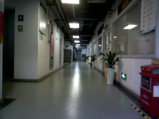
Appl. Sci. 2019, 9, 2105                                                                           2 of 17

often used LiDAR as the main sensor. Extended Kalman filter (EKF) was applied to estimate the
pose and of the robot [1], but the performance was not ideal. For some strong nonlinear systems,
this method will bring more truncation errors, which may lead to inaccurate positioning and mapping.
Particle filter approaches [2,3] were introduced because they can effectively avoid the nonlinear
problem, but it also leads to the problem of increasing the amount of calculation with the increase of
particle number. In 2007, Grisetti proposed a milestone of LiDAR-SLAM method called Gmapping [2],
based on improved Rao-Blackwellized particle filter (RBPF), it improves the positioning accuracy
and reduces the computational complexity by improving the proposed distribution and adaptive
re-sampling technique.
     As an effective alternative to probabilistic approaches, optimization-based methods are popular
in recent years. In 2010, Kurt Konolige proposed such a representative method called Karto-SLAM [3],
which uses sparse pose adjustment to solve the problem of matrix direct solution in nonlinear
optimization. Hector SLAM [4] proposed in 2011 uses the Gauss-Newton method to solve the problem
of scanning matching, this method does not need odometer information, but high precision LiDAR is
required. In 2016, Google put forward a notable method called Cartographer [5], by applying the laser
loop closing to both sub-maps and global map, the accumulative error is reduced.

1.2. Visual-SLAM
      Using visual sensors to build environment map is another hot spot for robot navigation. Compared
with LiDAR-SLAM, Visual-SLAM is more complex, because image carries too much information,
but has difficulty in distance measurement. Estimating robot motion by matching extracted image
features under different poses to build a feature map is a common method for Visual-SLAM.
      Mono-SLAM [6], proposed in 2007, is considered the origin of many Visual-SLAM. Extended
Kalman filter (EKF) is used as the back-end to track the sparse feature points in the front-end.
The uncertainty is expressed by a probability density function. From the observation model and
recursive calculation, the mean and variance of the posterior probability distribution are obtained.
Reference [7] used RBPF to realize visual-SLAM. This method avoids the problem of non-linear and has
high precision, but it needs a large number of particles, which increase the computational complexity.
PTAM [8] is a representative work of visual-SLAM, it proposed a simple and effective method to extract
key frames, as well as a parallel framework of a real-time tracking thread and a back-end nonlinear
optimization mapping thread. It is the first time to put forward the concept of separating the front and
back ends, leading the structure design of many SLAM methods.
      ORB-SLAM [9] is considered as a milestone of visual-SLAM. By applying Oriented FAST and
Rotated BRIEF (ORB) features and bag-of-words (BOW) model, this method can create a feature
map of the environment in real-time stably in many cases. Loop detection and closing via BOW is
an outstanding contribution of this work, it effectively prevents the cumulative error and can be quickly
retrieved after the tracking lost.
      In recent years, different from feature-based methods, some direct methods of visual-SLAM were
explored, by estimating robot motion through pixel value directly. Dense image alignment based on
each pixel of the images proposed in Reference [10] can build a dense 3D map of the environment.
The work in Reference [11] built a semi-dense map by estimating the depth values of pixels with
a large gradient in the image. Engel et al. proposed LSD-SLAM (Large-Scale Direct Monocular
SLAM) algorithm [12]. The core of LSD-SLAM algorithm is to apply a direct method to semi-dense
monocular SLAM, which is rarely seen in the previous direct method. Forster et al. proposed SVO
(Semi-Direct Monocular Visual Odometry) [13] in 2014, called “sparse direct method”, which combines
feature points with direct methods to track some key points (such as corners, etc.), and then estimates
the camera motion and position according to the information around the key points. This method
runs fast for Unmanned Aerial Vehicles (UAV), by adding special constraints and optimization to
such applications.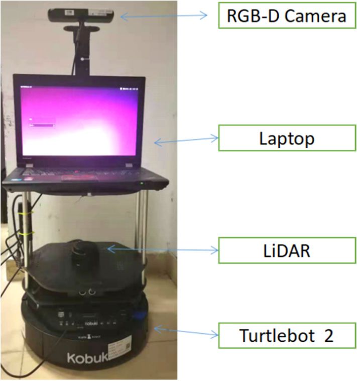
Appl. Sci. 2019, 9, 2105                                                                              3 of 17

     RGB-D camera can provide both color and depth information in its view field. It is the most
capable sensor for building a complete 3D scene map. Reference [14] proposes Kinect fusion method,
which uses the depth images acquired by Kinect to measure the minimum distance of each pixel in
each frame, and fuses all the depth images to obtain global map information. Reference [15] constructs
error function by using photo-metric and geometric information of image pixels. Camera pose is
obtained by minimizing the error function. Map problem is treated as pose graph representation.
Reference [16] is a better direct RGB-D SLAM method. This method combines the intensity error
and depth error of pixels as error functions, and minimizes the cost function to obtain the optimal
camera pose. This process is implemented by g2o. Entropy-based key frame extraction and closed-loop
detection method are both proposed, thus greatly reducing the path error.

1.3. Multi-Sensor Fusion
      Introducing assistant sensor data can improve the robustness of the SLAM system. Currently,
for LiDAR-SLAM and Visual-SLAM, the most commonly used assistant sensors are encoder and
Inertial Measurement Unit (IMU), which can provide additional motion data of the robot. SLAM
systems [2,5,17–20] with such assistant sensors usually perform better.
      In recent years, based on the works of LiDAR-SLAM and Visual-SLAM, some researchers have
started to carry out the research of integrating such two main sensors [21–25]. In [21], the authors applied
a visual odometer to provide initial values for two-dimensional laser Iterative Closets Point (ICP) on
a small UAV, and achieved good results in real-time and accuracy. In [22], a graph structure-based
SLAM with monocular camera and laser is introduced, with the assumption that the wall is normal to
the ground and vertically flat. [23] integrates different state-of-the art SLAM methods based on vision,
laser and inertial measurements using an EKF for UAV in indoor. [24] presents a localization method
based in cooperation between aerial and ground robots in an indoor environment, a 2.5D elevation
map is built by RGB-D sensor and 2D LiDAR attached on UAV. [25] provides a scale estimation and
drift correction method by combining mono laser range finder and camera for mono-SLAM. In [26],
a visual SLAM system that combines images acquired from a camera and sparse depth information
obtained from 3D LiDAR is proposed, by using the direct method. In [27], EKF fusion is performed
on the poses calculated by LiDAR module and vision module, and an improved tracking strategy is
introduced to cope with the tracking failure problem of Vision SLAM. As camera and LiDAR becoming
standard configurations for robots, laser-vision fusion will be a hot research topic for SLAM, because it
can provide a more robust result for real applications.

1.4. Problems in Application
      Generally speaking, LiDAR-SLAM methods build occupy grid map, which is ready for
path-planning and navigation control. However, closed-loop detection and correction are needed
for larger map building, and that is not easy for a grid map. Because the scan data acquired are
two-dimensional point cloud data, which have no obvious features and are very similar to each other,
the closed-loop detection based on scan data directly is often ineffective. And this flaw also extends to
fast relocation function when robot running with a given map. In the navigation package provided by
the Robot Operating System (ROS), the robot needs a manually given initial pose before automotive
navigation and moving. On the other hand, Most Visual-SLAM approaches generate feature maps,
which are good at localization, but not good for path-planning. RGB-D or 3D-LiDAR are capable of
building a complete 3D scene map, but it is limited in use because of high calculating or founding cost.
      For consumer robots, the cost of sensors and processing hardware is sensitive. Low-cost LiDAR
sensors become popular. However, to realize a robust low-cost navigation system is not easy work.
Because low-cost LiDAR sensors have much poorer performance in frequency, resolution and precision
than normal ones. In one of our previous work [28], we have introduced methods to improve the
performance of scan-matching for such low-cost LiDAR, however, that only works for adjacent poses.
The accumulating errors may usually grow too fast and cause failure to larger map building. To find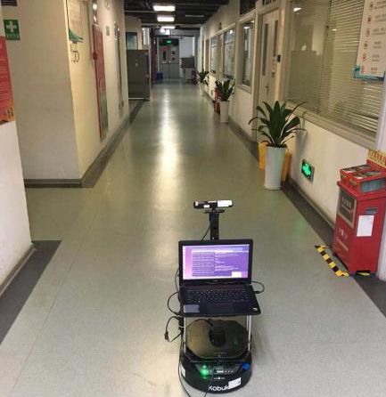
Appl. Sci. 2019, 9, 2105 4 of 17
Appl. Sci. 2019, 9, x FOR PEER REVIEW 4 of 17
an effective and robust SLAM and relocation solution with low computation cost and the low founding
building.
cost is stillTo find an effective
a challenging work for andcommercially-used
robust SLAM and service relocation solution with low computation cost
robots.
and the low founding cost is still a challenging work for commercially-used service robots.
1.5. The Contributions of this Paper
1.5. The Contributions of this Paper
This paper proposes a robust low-cost SLAM frame work, with the combination of low-cost LiDAR
This paper
and camera. proposes athe
By combining robust
laserlow-cost SLAM
points cloud dataframe work, feature
and image with thepoints
combination of low-cost
data as constraints,
aLiDAR and camera. method
graph optimization By combiningis usedthe laser points
to optimize cloudofdata
the pose and image
the robot. At thefeature pointsthe
same time, data
BoW as
constraints,
based a graph
on visual optimization
features is used for method is used to
loop closure optimizeand
detection, the then
pose the
of the robot.
grid mapAt the by
built samelasertime,
is
the BoW
further based on visual
optimized. Finally,features
a 2.5D map is used for loop both
presenting closure detection,
obstacles and and
occupy thenvision
the grid map built
feature is built,by
laser isisfurther
which ready foroptimized. Finally, a 2.5D map presenting both obstacles occupy and vision feature is
fast re-localization.
built,The
whichmainis contribution/advantages
ready for fast re-localization. of this paper are:
The main contribution/advantages of this paper are:
• Proposes a new low-cost laser-vision slam system. For graph optimization, a new cost-function
Proposes a new low-cost laser-vision slam system. For graph optimization, a new
considering both laser and feature constraints. We also added image feature-based loop-closure to
cost-function considering both laser and feature constraints. We also added image
the system to remove accumulative errors.
feature-based loop-closure to the system to remove accumulative errors.
• Proposes
Proposes a 2.5Da map, it is fast
2.5D map, it isinfast
re-localization and loop-closing,
in re-localization compared
and loop-closing, with feature
compared map,
with feature
it is ready for path-planning.
map, it is ready for path-planning.
The remaining
The remaining parts
parts ofof this
this paper
paper are are organized
organized as asfollows:
follows: Section
Section 22 introduces
introduces the
the slam
slam
framework based on graph optimization; Section 3 introduces the back-end
framework based on graph optimization; Section 3 introduces the back-end optimization and loop optimization and loop
closing method;
closing method; Section
Section 44 introduces
introduces the the 2.5D
2.5D map
map andand fast
fast relocation
relocation algorithm;
algorithm; Section
Section 55 isis the
the
experiment.; and Section 6 is the conclusion
experiment; and Section 6 is the conclusion part. part.
2. SLAM
2. SLAM Framework
Framework Based
Based on
on Graph
Graph Optimization
Optimization
A graph-based
A graph-based SLAM framework
framework could
could be
bedivided
dividedinto
intotwo
twoparts:
parts:Front-end and
Front-end back-end,
and as
back-end,
shown
as in in
shown Figure 1 below.
Figure 1 below.
Pose Update
Front-End
Constrains Back-End
Sensor
Data Input (Pose Estimation) (Optimization)
Poses
Figure1.1. A
Figure A general
general graph-based
graph-basedlight
lightdetection
detectionand
andranging
ranging(SLAM)
(SLAM)framework.
framework.
The
The front-end
front-end is
is mainly
mainly used
used toto estimate
estimate the the position
position andand pose
pose of
of the
the robot
robot byby sensor
sensor data.
data.
However, the observed data contain varying degrees of noise whether in images
However, the observed data contain varying degrees of noise whether in images or in laser. or in laser. Especially
for low-cost for
Especially LiDAR and cameras.
low-cost LiDAR The andnoise will lead
cameras. Thetonoise
cumulative errors
will lead toincumulative
pose estimation,
errorsand
in such
pose
errors will increase with time. Through filtering or optimization algorithms, the back-end
estimation, and such errors will increase with time. Through filtering or optimization algorithms, part can
eliminate the cumulative errors and improve the positioning and map accuracy.
the back-end part can eliminate the cumulative errors and improve the positioning and map
In this paper, graph optimization is used as the back-end, and the error is minimized by searching
accuracy.
the descending gradient
In this paper, graphthrough nonlinear
optimization optimization.
is used Graph and
as the back-end, optimization
the error simply describes
is minimized by
an optimization problem in the form of a graph. The node of the graph represents
searching the descending gradient through nonlinear optimization. Graph optimization simply the position and
attitude,
describesandanthe edge represents
optimization the constraint
problem in the form relationship
of a graph.between the position
The node and the
of the graph attitude and
represents the
the observation. The sketch map of graph optimization is shown in Figure 2.
position and attitude, and the edge represents the constraint relationship between the position and
the attitude and the observation. The sketch map of graph optimization is shown in Figure 2.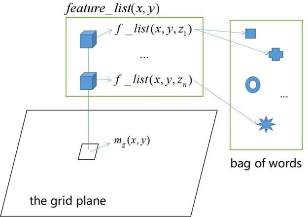
Appl. Sci.
Appl. Sci. 2019,
2019, 9,
9, 2105
x FOR PEER REVIEW 55 of
of 17
17
Appl. Sci. 2019, 9, x FOR PEER REVIEW 5 of 17
Figure 2. Sketch map of graph optimization.
Figure 2. Sketch map of graph optimization.
In Figure 2, X represents the position and pose of the robot, and Z represents the observation.
In thisInpaper,
Figure the
2,robot observes the
X represents the external
positionenvironment
and pose of the through
robot, both
andLiDAR and camera.
Z represents As a result,
the observation.
ZIncould be a combination of three-dimensional spatial feature points
this paper, the robot observes the external environment through both LiDAR and camera. detected by camera or obstacle
As a
points
result, Z could be a combination of three-dimensional spatial feature points detected by cameraare
detected by LiDAR. Matching result and errors of visual feature points and scan data or
an essential part to generate the Figure
nodes 2.and
Sketch map of for
constrain graph optimization.
graph optimization.
obstacle points detected by LiDAR. Matching result and errors of visual feature points and scan
dataFor theessential
are an matching of to
part visual
generatefeature points,and
the nodes theconstrain
error is for usually
graphrepresented
optimization.by re-projection
In
error.For Figure
Thethe 2, X
calculation represents the position and pose of the robot, and Z represents theto
observation.
matchingofofre-projection
visual feature error needsthe
points, to give
error two cameras
is usually corresponding
represented adjacent
by re-projection
In this two-dimensional
frames, paper, the robot coordinates
observes theofexternal
matched environment
feature points through
in two both
imagesLiDAR
and and camera. As a
three-dimensional
error. The calculation of re-projection error needs to give two cameras corresponding to adjacent
result, Z could
coordinates be a combination
of corresponding of three-dimensional
three-dimensional space points.spatial feature points detected by camera or
frames, two-dimensional coordinates of matched feature points in two images and
obstacle
As points
shown in detected
Figure 3, by
for LiDAR.
the Matching
feature point result
pairs p and
and perrors of visual feature points and scan
three-dimensional coordinates of corresponding three-dimensional 1 2 in adjacent
spaceframes,
points.a real-world spatial
data Pare
point an essential part
corresponding to p1tocould
generate the nodes
be localized at and
first,constrain
and then for P isgraph optimization.
re-projected onto the latter frame
For the matching of visual feature points, the error is usually
to form the feature point position p̂2 of the image. Due to the error of position and pose represented by re-projection
estimation,
error. The calculation of re-projection error needs to give two cameras
the existence of p̂2 and p2 is not a coincidence. The distance between these two points could be corresponding todenoted
adjacent
frames, two-dimensional coordinates of matched feature points
as a re-projection error. Pure vision SLAM usually extracts and matches feature points, approaches in two images and
three-dimensional coordinates of corresponding three-dimensional space
like EPnP [29] can be applied to estimate the pose transformation (R, t) of adjacent frames. Where R points.
represents the rotation matrix, and t represents the transformation matrix.
Figure 3. The re-projection error.
As shown in Figure 3, for the feature point pairs p1 and p 2 in adjacent frames, a real-world
p1 could
spatial point P corresponding to Figure 3. Thebe localized at
re-projection first, and then P is re-projected onto
error.
the latter frame to form the feature point
Figureposition p̂ 2 of theerror.
3. The re-projection image. Due to the error of position and
According to Figure 3, the re-projection errors could be calculated as follows:
poseFirstly,
estimation, the the
existence 0 , Y0 , p
of p̂ 2 Xand is not
20 ] of a coincidence. point
0 (corresponding The distance betweencoordinate,
these two
As showncalculate
in Figure for the [feature
3D3,position Zpoint Ppairs of P) inframes,
p1 and p 2 in adjacent camera a real-world
points could
through be denoted
the pose as a re-projection
and transformation relationerror. [R,t]: Pure vision SLAM usually extracts and matches
feature point P
spatial points, corresponding
approaches to p[29]
like EPnP 1 could
can be be applied
localizedtoatestimate
first, and posePtransformation
thethen is re-projected
( Ronto
, t)
the latter frame to form the feature
of adjacent frames. Where R represents
0
point
P = RP position
the+rotation p̂ 2 , matrix,
t = [X 0 of 0 the T
0 image. Due to the error of position and
Y , Z ] . and t represents the transformation (1)
pose estimation, the existence of p̂ 2 and p 2 is not a coincidence. The distance between these two
matrix.
Then, get the normalized
According coordinate Pc : errors could be calculated as follows:
points could betodenoted
Figure 3,asthe re-projection
a re-projection error. Pure vision SLAM usually extracts and matches
Firstly, calculate the 3D position
feature points, approaches likePEPnP [ X
[29] can ' ,TY be
' , Zapplied
' ]0 of0 P’to
0 (corresponding
estimate
0 T the posepoint of P) in camera
transformation ( R(2)
, t)
c = [uc , vc , 1] = [X /Z , Y /Z , 1] .
coordinate, through the pose and transformation relation [ R, t ] :
of adjacent frames. Where R represents the rotation matrix, and t represents the transformation
matrix.
Based on camera parameters ( fx , f y , cx , c y ), the re-projected Tpixel coordinate p̂2 = (us , vs ) could be
According
calculated as:
P' = RP +errors
to Figure 3, the re-projection
t = [X ',Y ', Z ' ] .
could be calculated as follows:
(1)
(
Firstly, calculate the 3D position [ Xus' ,= Y 'f,xZuc' ]+ of
cx P’ (corresponding point of P) in camera
Then, get the normalized coordinate Pc : . (3)
coordinate, through the pose and transformation vs = f y relation
vc + c y [ R, t ] :
Pc = [uc , vc ,1]T = [ X ' / Z ' , Y ' / ZT ' ,1]T . (2)
P' = RP + t = [ X ' , Y ' , Z ' ] . (1)
Then, get the normalized coordinate Pc :
Pc = [uc , vc ,1]T = [ X ' / Z ' , Y ' / Z ' ,1]T . (2)could be calculated as:
u s = f x uc + c x
. (3)
vs = f y vc + c y
Appl. Sci. 2019, 9, 2105 6 of 17
Finally, if there are n feature points matched between two frames, the re-projection error is:
n
1 between two
1 =
Finally, if there are n feature pointsematched
2
|| pi − pˆ i ' ||22 . frames, the re-projection error is: (4)
i =1
n
1X 0 2
Compared with the visual error, the e =
1 laser scan pi − p̂matching
i 2. error is much simpler to obtain. (4)
2
i = 1
LiDAR-SLAM usually needs scan matching to realize the estimation of pose transformation of
adjacent frames. with
Compared The estimated error, the laser( Rscan
the visualtransformation , t ) cannot guarantee
matching error isthat all the
much laser data
simpler in the
to obtain.
previous frameusually
LiDAR-SLAM completely
needs coincide with to
scan matching therealize
laser the
dataestimation
in the latter frame
of pose according toofthe
transformation pose
adjacent
transformation. The error
frames. The estimated could be calculated
transformation as:
(R, t) cannot guarantee that all the laser data in the previous
frame completely coincide with the laser data n in the latter frame according to the pose transformation.
2
The error could be calculated as: e2 = n M i − ( RSi + t ) 2 , (5)
i =1
X
2
e2 = kMi − (RSi + t)k2 , (5)
where n is the number of matched scan points, M is the source scan point set and S is the scan
i = 1
point set
where n isofthe
annumber
adjacentofframe.
matched scan points, M is the source scan point set and S is the scan point set
With multiple
of an adjacent frame. adjacent frame pairs get by Visual-SLAM or LiDAR-SLAM, the united
re-projections errors
With multiple of different
adjacent frameframe pairs
pairs get bycould be minimized
Visual-SLAM for optimizing
or LiDAR-SLAM, multiple
the united poses.
re-projections
errors of different frame pairs could be minimized for optimizing multiple poses.
3. The SLAM Framework of Low-Cost LiDAR and Vision Fusion
3. The SLAM Framework of Low-Cost LiDAR and Vision Fusion
Base on the framework and key parts introduced in section 2, this paper proposes a new SLAM
Base onof
framework thelow-cost
framework and key
LiDAR andparts introduced
vision fusion. in
In Section 2, this paper
the framework, forproposes a new SLAM
the back-end graph
framework of low-cost
optimization, LiDARerror
a new united and vision fusion.
function In the framework,
of combining for the
visual data back-enderror
matching graph optimization,
and laser data
a new united
matching error
error is function of combining
introduced. Meanwhile,visual
in data
ordermatching
to solveerror
the and laser data
problem matching
of loop error of
detection is
introduced. Meanwhile, in order to solve the problem of loop detection of traditional
traditional LiDAR-SLAM, a loop detection method is added, by introducing and visual data and LiDAR-SLAM,
a loop detection
bag-of-words. method
The is added,
integrated SLAM by framework
introducingcombining
and visualwith
data laser
and bag-of-words.
and vision data Theisintegrated
shown in
SLAM framework
Figure 4 below: combining with laser and vision data is shown in Figure 4 below:
Laser Scan Scan
Data Matching MAP
Update
Poses and Pose Graph With Scan
Constrains Optimization Data and
Feature
Image Feature Pose Points
Data Extraction Estimation
Bag of Close Loop
Matching
Words Detection
The proposed SLAM framework.
Figure 4. The
In the
In the framework,
framework,bothboththe
thelaser
laserdata
data and image
and imagedata cancan
data get get
the robot posepose
the robot estimation. For laser
estimation. For
data, scan-to-scan or scan-to-map methods can be applied to estimate current robot pose.
laser data, scan-to-scan or scan-to-map methods can be applied to estimate current robot pose. For For image
data, we
image canwe
data, usecan
the use
ORBthefeature
ORB for image
feature forfeature
imagedetection and generate
feature detection the bag ofthe
and generate words.
bag ofMethods
words.
like EPnPlike
Methods [24]EPnP
could[24]
be applied
could betoapplied
estimate tothe pose transformation
estimate of adjacent
the pose transformation offrames.
adjacent frames.
3.1. United Error Function
The traditional error function for the matching of image data or scan data is given in Section 2.
In this part, for further optimization and mapping procedure, we introduce a united error function
with the fusion of image data and scan data.Appl. Sci. 2019, 9, 2105 7 of 17
Considering two adjacent robot poses with an initial guess of translation and rotation parameters
[R,t], which could get through scan matching, image feature matching or even encoder data individually.
Based on the error formulas introduced in Section 2, the united error function could be expressed as:
m n
X 1 X
e=β pi − C(RPi−1 + t)) + (1 − β)α (P j − (RP j−1 + t)) , (6)
Zi−1
i=1 j=1
where m is the number of matched features; n is the number of corresponding scan points; C is the
camera parameter matrix;pi is the image position of feature; P j is the scan point position; α is a parameter
for unit conversion of the image pixel error and distance error, it is mainly judged by camera resolution
and laser ranging range; β is the parameter for balancing the two measurements, it takes value between
(0,1). It is mainly judged by the two sensors’ reliability and precision, for example, if the robot is
working in an environment full of image features, β can be larger so that we consider visual input more
important. In contrast, if the scene is better for laser processing, β can be smaller.
(R, t) can be written in an algebra form, and the Lie Algebraic transformation formula is:
RP + t = exp(ξ̂)P. (7)
Then the error function could be reformulated as a Lie algebra form:
m n
X 1 X
e = F(ξ) = β pi − C exp(ξ̂)Pi−1 ) + (1 − β)α (P j − exp(ξ̂)P j−1 ) (8)
Zi−1
i=1 j=1
It is a function with the variable, ξ. For K pairs of multiple poses with their transformation
relations, the total error could be written as:
K
X K
X
E= ei = Fi (ξi ), (9)
i=1 i=1
and such error can be minimized to find better transformations and rotations between multiple poses.
3.2. Pose Graph Optimization
Due to the errors and noise of sensor measurements, the best matching of two adjacent poses may
not be the best for the whole map. By unitizing a series of relative poses, the pose graph optimization
could be applied for minimizing the errors during the SLAM process. In our approach, the robot pose
set x is regarded as the variable to be optimized, and the observations are regarded as the constraints
between the poses.
The robot pose set x is:
x = [x1 , x2 , x3 , . . . , xk ]T . (10)
Based on the Lie Algebraic transformation set ξ, robot pose set x is related to transformation set of
ξ by:
x = h(ξ). (11)
Which also could be written as:
ξ = h−1 (x). (12)
As a result, the total error of K pairs of related poses could be rewritten as:
K
X K
X
E= ei = Fi (ξi ) = f (x). (13)
i=1 i=1Appl. Sci. 2019, 9, 2105 8 of 17
The target of pose graph optimization is to find a proper set x, so that the error f (x) is minimized.
Correspondingly, ∆x is the increment of the x of the global independent variable. Therefore, when the
increment is added, the objective function is:
k
1 2 1X 2
f (x + ∆x) ≈ f (xt ) + Jt ∆xt , (14)
2 2
t=1
where J represents the Jacobian matrix, which is the partial derivative of the cost function to the
variables, k is the number of poses to be optimized, and the number of postures between the current
frame and the loop frame is the global optimization.
Position and pose optimization can be regarded as the least square problem. The commonly used
methods to solve the least square problem are Gradient Descent method, Gauss Newton method [30]
and Levenberg-Marquadt (L-M) method [31]. The L-M method is a combination of Gadient Descent
method and Gauss Newton method. This paper uses the L-M method to solve the least square problem.
According to L-M method and formula (14), in each iteration step, we need to find:
1 2 2
min f (xi ) + J (xi )∆xi s.t. I∆xi ≤ µ, (15)
∆xi 2
where µ is the radius of the searching area (here we judge the area is a space sphere) in each step. The
problem could be changed to solve the following incremental equation:
( J (x)T J (x) + λI )∆x = −J (x)T f (x), (16)
where J represents the Jacobian matrix, and λ is the Lagrange multiplier. As in each iteration step, x is
known, let H = J (x)T J (x) and g = −J (x)T f (x), it could be rewritten as:
(H + λI)∆x = g. (17)
As L-M method could be regarded as a combination of Gadient Descent method and Gauss
Newton method in the formula (17), it could be more robust to get a reliable ∆x even if H is not
invertible. By solving the above linear equation, we can obtain ∆x, and then iterate ∆x to obtain
x corresponding to the minimum objective function, that is robot pose. Generally speaking, the
dimension of H is very large, and the complexity of matrix inversion is O(n3 ). However, because H
contains the constraints between poses, and only the adjacent posed have direct constraints, most of
the elements are 0. H is sparse and shaped like an arrow. The calculation of (17) could be accelerated.
In practice, the pose graph optimization problem could be solved through tools like g2o [32] or
ceres [33], with given error function and initial value. In our work, we apply g2o to solve this problem.
The error function is formula (8), and the initial value of x is obtained mainly through scan matching.
3.3. Loop Detection
Loop detection is a core problem in SLAM. Recognizing the past places and adding loop pose
constraints to the pose graph can effectively reduce the cumulative error and improve the positioning
accuracy. SLAM algorithms based on LiDAR are often unable to detect the loop effectively, because
scan data can only describe the obstacle structure on the LiDAR installation plane, which usually lack
of unique features of the scene. In other words, there may be multiple places that have very similar
scan data to be detected, such as long coordinator, office workplace card, rooms with similar structure,
etc. The rich texture features of visual images can just make up for this defect in our work.
In this paper, BoW is applied to construct the dictionary corresponding to the key-frames by
visual features. Because the number of images captured by building indoor maps is too large, and the
adjacent images have a high degree of repeatably, the first step is to extract the key-frames. The keyAppl. Sci. 2019, 9, 2105 9 of 17
frame selection mechanism is as follows: (1) It has passed 15 frames since the last global relocation;
(2) the distance from the previous key-frame has been 15 frames. (3) key frames must have tracked at
least 50 three-dimensional feature points.
Among them, (1) (2) is the basis of its uniqueness, because in a short period of time the
characteristics of the field of vision will not change significantly (3) to ensure its robustness, too few
map points will lead to an uneven calculation error.
For each key-frame, the ORB image features and their visual words in BoW dictionary are
calculated and saved as a bag of features. As a result, a key-frame stores the robot pose and bag
of features, as well as the scan data obtained in that pose. It should be denoted that the key-frame
here is applied for loop detection or relocation, the robot pose of each key-frame is updated after
global optimization.
During the loop detection procedure, for an incoming image frame, the bag of feature is calculated
and matched with all possible previous key-frames (possible means the key-frame should be a period
of time before, and close enough in an estimated pose during SLAM procedure). When the current
image frame is sufficiently similar to a key frame image by match the bag of feature, closing loop
possibility is considered. Then, the current frame and that key frame are matched by both the scan
data and image data, and the error in formula (6) is also calculated. If the matching error is small
enough, the loop is confirmed and the matching result is added as constraints to the graph optimization
framework, so that the accumulative errors can be eliminated.
4. 2.5D Map Representation and Relocation
In this part, we introduce a new expression of the 2.5D map, based on the scan data and visual
data collected during the proposed method, as well as a fast relocation approach via the map.
4.1. Traditional Grid Map and Feature Map
Occupy grid map is wildly used in LiDAR-SLAM, it is a simple kind of 2D map that represents
the obstacles on the LiDAR plane:
M grid = {m g (x, y)}, (18)
where m g (x, y) denotes the possibility if the grid (x, y) is occupied. Generally, the value of m g (x, y) can
be 1 (the grid (x, y) is occupied) or 0 (the grid (x, y) is not occupied).
Feature map is another kind map generated by most feature-based Visual-SLAM approaches, it
can be represented as:
M f eature = { f (x, y, z)}, (19)
where f (x, y, z) denotes that on the world position (x, y, z), there is a feature f (x, y, z), for real
applications, f (x, y, z) could be a descriptor to the feature in a dictionary like BoW.
While Visual-SLAM processing, key-frames with bag-of-feature description and poses at where
they were observed are usually stored as an accessory for feature maps. For relocation applications,
searching and matching in key-frames can greatly improve the processing speed and reliability.
As a result, a feature map is a sparse map which only has value on the position which has features.
This makes a feature map is reliable for localization, but not good for navigation and path-planning.
4.2. Proposed 2.5D Map
Based on previous sections, the obstacle detected in the 2D laser plane and the image features
detected by the camera can be aligned in one map, which can be represented as:
M = {m(x, y)}, (20)
n o
m(x, y) = m g (x, y), f eature_list(x, y) , (21)features. This makes a feature map is reliable for localization, but not good for navigation and
path-planning.
4.2. Proposed 2.5D Map
Based
Appl. Sci. 2019, on previous
9, 2105sections, the obstacle detected in the 2D laser plane and the image features
10 of 17
detected by the camera can be aligned in one map, which can be represented as:
M =in{m
where f eature_list(x, y) represents the features ( xcorresponding
the , y )} , (20)
vertical space of the grid (x, y).
If there is no feature detected above grid (x, y), f eature_list(x, y) = null.
m( x, y ) = {mg ( x, y ), feature _ list ( x, y )} , (21)
A general form of f eature_list(x, y) could be:
where feature _ list ( x , y ) represents the features in the corresponding vertical space of the grid
f eature_list(x, y) = f _list(x, y, z1 ), f _list(x, y, z2 ), . . . , f _list(x, y, zn ) , (22)
( x, y ) . If there is no feature detected above grid ( x, y ) , feature _ list ( x , y ) = null .
A general
where 2 , . . . zof
z1 , zform featurethe
n denotes _ list ( x , y )height
vertical couldon be:which there is an image feature located above the
grid (x, y), and f _list(x, y, z) is a list pointing to features in the feature bag. It should be denoted this
expression is quite feature_li
differentst(x,y) ={f _ list(x,y,z
from traditional 1 ),f _
methods, aslist(x,y,z 2 ),...be
there could ,f multiple
_ list(x,y,z n )} , on a single
features (22)
space point (x, y, z). That seems odd, but necessary in practice. When the camera is moving while
where z1,z2 ,...zn denotes the vertical height on which there is an image feature located above the
SLAM, the image feature of one place is actually changing because of the huge change of visual angles
and ( x, y ) , and fIn_the
gridilluminations. listhistory
( x , y , z )of isimage
a listprocessing,
pointing to features in
researchers thebeen
have feature bag. It with
struggling should be
such
denotedand
changes thisdeveloped
expressionvarious
is quite different
features thatfrom traditionaltomethods,
are “invariant” as theretransformation
scaling, rotation, could be multipleand
features on a single space point ( x , y , z ) . That seems odd, but
illumination, so that they can track the same place of the object and do more other works. In the necessary in practice. When the
expression of the proposed
camera is moving 2.5D map,
while SLAM, the imageconsideringfeature theofhuge changeisof
one place visual angles
actually changingandbecause
illuminations
of the
while
huge change of visual angles and illuminations. In the history of image processing, researchers have
SLAM, the feature in one place may change greatly, as a result, we assume one place could have
multiple features.with such changes and developed various features that are “invariant” to scaling,
been struggling
As shown
rotation, in Figure and
transformation 5, a 2.5D Map combing
illumination, so thatwiththeydense
can trackobstacle
the samerepresentation
place of theonobject
the 2D
andgrid
do
plane
more and
other sparse
works. features
In therepresentation
expression ofinthe 3Dproposed
space above 2.5Dthemap,
planeconsidering
could be obtained,
the huge through
changetheof
combination
visual anglesand andoptimization
illuminationswith while LiDARSLAM, andthecamera
featuresensors. A listmay
in one place of key-frames with as
change greatly, poses and
a result,
visual wordsone
we assume extracted whilehave
place could SLAM processing
multiple is also attached to the map.
features.
Figure 5. The
Figure5. The expression
expression of
of the
the proposed
proposed2.5D
2.5Dmap.
map.
In
Asthe map,in
shown inFigure
order to
5, simplify the combing
a 2.5D Map calculation,
with the resolution
dense obstacleis uninformed
representation byon
thethe
grid2Dmap,
grid
for example,
plane the smallest
and sparse featuresgrid cell could bein5 3D
representation × 5 cmabove
cm space × 5 cm.
theInplane
that case,
couldthere may be multiple
be obtained, through
feature points with
the combination anddifferent feature with
optimization valueLiDAR
detected
andin camera
one cell.sensors.
That situation
A list ofiskey-frames
also considered
with in the
poses
map representation.
and visual words extracted while SLAM processing is also attached to the map.
In the map, in order to simplify the calculation, the resolution is uninformed by the grid map,
4.3. Relocation with Proposed 2.5D Map
for example, the smallest grid cell could be 5 cm × 5 cm × 5 cm. In that case, there may be multiple
In real applications, although the robot already has the environment map, it may usually lose its
location. Such a situation happens when the robot starts on an unknown position, or was kidnapped
by a human (blocking the sensors and carry it away) while working. Relocation is required, and its
speed and the successful rate have a great influence on the practicability of a mobile robot system.
Currently, for the grid map created by LiDAR-SLAM approaches, Montecalo and particle
filter-based method is wildly applied to find the robot pose. However, because the scan data carries too
little unique information of the environment, it may take a long time for the robot to find its location.
On the other hand, image information is rich enough for fast place finding. In this paper, with the aid
of image features and BoW, a fast relocation algorithm with our map is as follows:Currently, for the grid map created by LiDAR-SLAM approaches, Montecalo and particle
filter-based method is wildly applied to find the robot pose. However, because the scan data carries
too little unique information of the environment, it may take a long time for the robot to find its
location. On the other hand, image information is rich enough for fast place finding. In this paper,
with the aid of image features and BoW, a fast relocation algorithm with our map is as follows:
Appl. Sci. 2019, 9, 2105 11 of 17
Firstly, extract current image features, calculate the bag-of-features (visual words) with BoW;
Secondly, List all the previous key-frames with poses in map which shares visual words with
current image,
Firstly, andcurrent
extract find n image
best match key-frames
features, calculate with ranking score (visual
the bag-of-features through BoW with
words) searching;
BoW;
Thirdly, for
Secondly, Listnall
best
thematch key-frames,
previous key-framesletwith
their poses
poses in as
mapinitial
which guess forvisual
shares particles;
words Finally, apply
with current
particleand
image, filter
findbased method
n best to find bestwith
match key-frames robot pose, score
ranking the error function
through BoW could be formula
searching; Thirdly,(6)
forin n
section 3.
best match key-frames, let their poses as initial guess for particles; Finally, apply particle filter based
method to find best robot pose, the error function could be formula (6) in Section 3.
5. Experiment
5. Experiment
The experiment is divided into three parts. In the first part, a comparative experiment of
fixed-point positioning
The experiment accuracy
is divided isthree
into carried out In
parts. inthe
a small rangea comparative
first part, of scenes. The traditionaloflaser
experiment SLAM
fixed-point
based on graph optimization, the visual SLAM based on orb feature point extraction
positioning accuracy is carried out in a small range of scenes. The traditional laser SLAM based and the laser
vision
on method
graph proposedthe
optimization, in visual
this paper
SLAM is used
based toon
collect positioning
orb feature pointdata. In the and
extraction second
the part,
laser avision
large
scene loop
method experiment
proposed in thisispaper
carried out totoverify
is used collectwhether the proposed
positioning data. In themethod
secondcan effectively
part, solveloop
a large scene the
problem of map
experiment closure
is carried outintolaser
verifySLAM.
whetherIn the
the last part, we
proposed load the
method canbuilt map for
effectively the the
solve re-localization
problem of
experiment.
map closure in laser SLAM. In the last part, we load the built map for the re-localization experiment.
5.1. Experimental Platform
5.1. Experimental Platform and
and Environment
Environment
The
The experiment
experimentwas
wascarried outout
carried on aonrobot platform
a robot based based
platform on Turtlebot 2, equipped
on Turtlebot with a notebook,
2, equipped with a
anotebook,
LiDAR and an RGB-D camera. The notebook has Intel Core i5 processor and 8G
a LiDAR and an RGB-D camera. The notebook has Intel Core i5 processor and 8G memory, running on
Ubuntu 14.04 + ROS Indigo system. The robot platform is shown in Figure 6:
memory, running on Ubuntu 14.04 + ROS Indigo system. The robot platform is shown in Figure 6:
Figure 6. The robot platform for the experiment.
The LiDAR is RPLIDAR-A2 produced by SLAMTEC company. It is a low-cost LiDAR for service
robotics, which has a 360◦ coverage field and range of up to 8 m. The key parameters are listed in
Table 1. It should be noted that the parameters are taken under the ideal situation, and being a low-cost
LiDAR, the data collected from it is usually much poorer than expensive ones in a real scene.
Table 1. The key parameters of RPLidar-A1.
Measuring Distance Ranging Accuracy Angle Range Angle Resolution Frequency
0.15–12 m 0.001 m 0–360◦ 0.9◦ 10
The RGB-D camera is Xtion-pro produced by ASUS company. The effective range of depth
measurement is 0.6–8 m, the precision is 3 mm, and the angle of view of the depth camera can reach
horizontal 58◦ and vertical 45.5◦ .
With the robot platform, we have collected several typical indoor databases in the “rosbag” format,
which is easy to read for ROS. For each database, it contains sensor data obtained by the robot while it is
running in a real scene, including odom data, laser scan, color image and depth image. Figure 7 showsThe RGB-D camera is Xtion-pro produced by ASUS company. The effective range of depth
measurement is 0.6–8 m, the precision is 3 mm, and the angle of view of the depth camera can reach
horizontal 58°and vertical 45.5°.
With the robot platform, we have collected several typical indoor databases in the “rosbag”
format, which
Appl. Sci. 2019, is easy to read for ROS. For each database, it contains sensor data obtained by
9, 2105 the
12 of 17
robot while it is running in a real scene, including odom data, laser scan, color image and depth
image. Figure 7 shows one example of the database. Where Figure 7a displays the robot in the
one example ofFigure
environment; the database.
7b shows Where
the Figure 7a displays
scan data theinrobot
obtained in the environment;
the place; Figure
Figure 7c is the RGB7b image;
shows
the scan data obtained
Figure 7d is the depth image. in the place; Figure 7c is the RGB image; Figure 7d is the depth image.
(a) (b)
(c) (d)
Figure 7. One example
example of
of the
thedatabase:
database:(a)
(a)The
Therobot
robotininthe
theenvironment;
environment;(b)(b)
scan data
scan obtained
data in the
obtained in
scene;
the (c) the
scene; RGBRGB
(c) the image; (d) the
image; (d) depth image.
the depth image.
Different experiments
Different experimentswere
weretaken
takentotoevaluate
evaluatethe performance
the performance of mapping
of mapping andand
relocation. For For
relocation. the
mapping, the methods for comparison include Karto-SLAM [3], orb-SLAM [9] and this
the mapping, the methods for comparison include Karto-SLAM [3], orb-SLAM [9] and this paper. paper. For the
relocation
For with s map,
the relocation with we compared
s map, our method
we compared ourwith the Adaptive
method with theMonte CarloMonte
Adaptive Localization
Carlo
(AMCL) [34]. In the experiments, the parameter β
Localization (AMCL) [34]. In the experiments, the parameter β of formula (6) and (8) is set to
of formulas (6) and (8) is set to 0.2, by considering
the precision and reliability of the two main sensors in the environment.
0.2, by considering the precision and reliability of the two main sensors in the environment.
5.2. Experiment of Building the Map
5.2. Experiment of Building the Map
Firstly, in order to evaluate the positioning accuracy while mapping, we manually marked
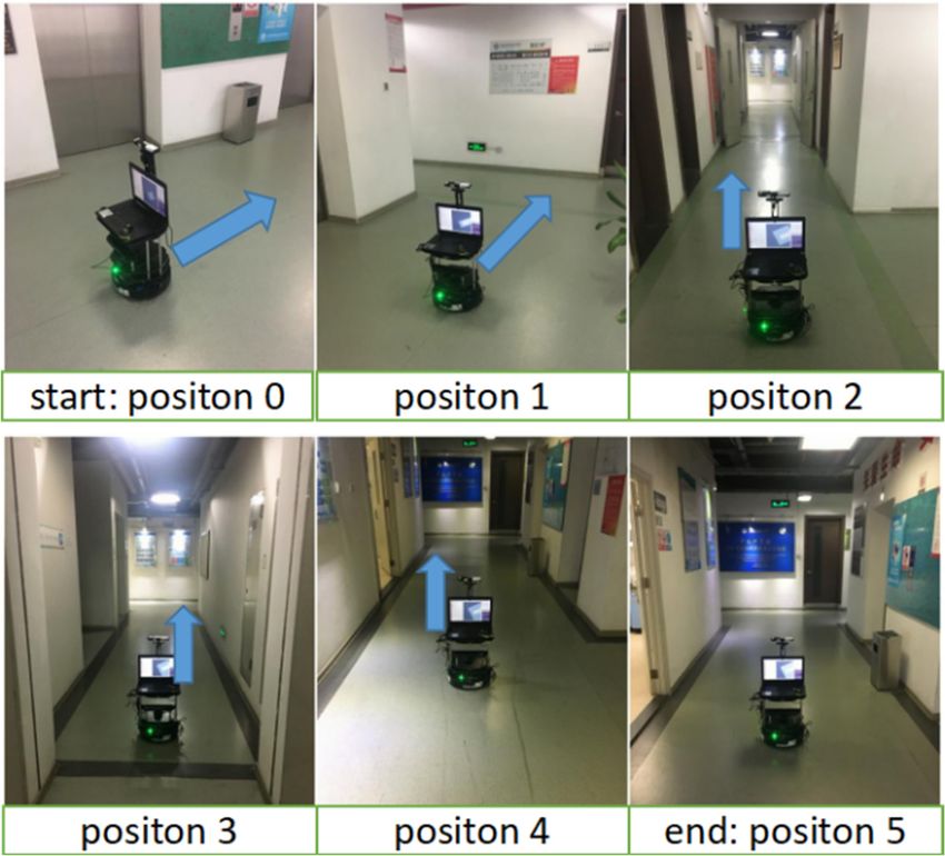
6 positions in a real scene, as shown in Figure 8. The start point position 0 is specified as the original
point (0,0) in the world coordinate system. As shown in Figure 8, the robot started from position 0 and
stopped at position 5, and the blue arrow in each picture is the robot’s moving direction. Table 2 shows
the result of positioning in the SLAM system from position 1 to position 5.Firstly, in order to evaluate the positioning accuracy while mapping, we manually marked 6
positions in a real scene, as shown in Figure 8. The start point position 0 is specified as the original
point (0,0) in the world coordinate system. As shown in Figure 8, the robot started from position 0
and stopped
Appl. Sci. 2019, 9,at position 5, and the blue arrow in each picture is the robot’s moving direction.13
2105 Table
of 17
2 shows the result of positioning in the SLAM system from position 1 to position 5.
Figure 8. The marked positions of the robot.
As can
canbebeseen
seenfrom Table
from 2, for2,both
Table for methods, the initial
both methods, the error of error
initial positioning is small. However,
of positioning is small.
while the robot was running further, the error increases with distance. Sooner or later,
However, while the robot was running further, the error increases with distance. Sooner or later, such error will
be
suchtooerror
largewill
to bebeignored,
too largeandtofinally cause failure
be ignored, to mapping.
and finally Such atosituation
cause failure mapping. may become
Such worth
a situation
for
maya become
low-costworth
LiDAR. forThat’s why we
a low-cost need That’s
LiDAR. a loop why
closing
wemodule for thr
need a loop SLAMmodule
closing system.for thr SLAM
system.
Table 2. The positioning result while Simultaneous Localization and Mapping (SLAM).
Table 2. The positioning result while Simultaneous Localization and Mapping (SLAM).
Position Number Real Position (m) Karto-SLAM (m) Our Method (m)
Position
1 Number Real Position
(3,0) (m) Karto-SLAM (m)
(2.995,−0.002) Our (2.994,−0.003)
Method (m)
2 1 (3,0)
(6,0) (2.995,−0.002)
(5.987,−0.003) (2.994,−0.003)
(5.990,−0.005)
3 2 (6,0)
(6,−8) (5.987,−0.003)
(6.025,−8.032) (5.990,−0.005)
(6.019,−8.021)
(6.025,−8.032) (6.019,−8.021)
4 3 (6,−8)
(6,−16) (6.038,−15.954) (6.028,−15.973)
(6.038,−15.954) (6.028,−15.973)
5 4 (6,−16)
(3,−16) (2.949,−15.946) (2.951,−15.965)
5 (3,−16) (2.949,−15.946) (2.951,−15.965)
We
We diddidfurther
furthermapping
mapping experiment in a real
experiment in scene
a realcompared with Karto-SLAM
scene compared and Orb-SLAM.
with Karto-SLAM and
The result is shown
Orb-SLAM. in Figure
The result 9. Figure
is shown 9a is the
in Figure result of
9. Figure 9aKarto-SLAM, theKarto-SLAM,
is the result of blue points are thethe estimated
blue points
robot
are theposition
estimated during
robotSLAM.
positionBecause
during of the growing
SLAM. Because cumulative
of the growingerror, the starting
cumulative point
error, the and the
starting
ending
point and point
the in the red
ending coilincannot
point the redbecoil
fused together,
cannot the together,
be fused mappingthe failed. Figure
mapping 9b isFigure
failed. the feature
9b is
map constructed
the feature by orb-SLAM.
map constructed It should beItdenoted
by orb-SLAM. should bethat orb-SLAM
denoted that is easy to lose
orb-SLAM tracking,
is easy and
to lose the
track,
robot should run and turn very slow while building the map. When tracking is lost,
and the robot should run and turn very slow while building the map. When losing track, it needs a it needs a manual
operation to turn back
manual operation to to findback
turn previous key-frames.
to find previous As a result, orb-SLAM
key-frames. can’torb-SLAM
As a result, work directly with
can’t our
work
recorded rosbag
directly with ourdatabases. Figure 9c
recorded rosbag is the gridFigure
databases. map part
9c isofthe
thegrid
proposed
map partmethod,
of thethe green points
proposed method,are
the robot
greedpositions
points areestimated
the robotduring SLAM.estimated
positions Because ofduring
the effective
SLAM.loop detection
Because andeffective
of the optimization,
loop
the map isand
detection much better than compared
optimization, the map ismethods. The than
much better final 2.5D map showing
compared methods.both
Thegridfinaland
2.5Dfeature
map
point
showingis shown in Figure
both grid 10.
and feature point is shown in Figure 10.Appl. Sci. 2019, 9, 2105 14 of 17
Appl.
Appl. Sci.
Sci. 2019,
2019, 9,
9, xx FOR
FOR PEER
PEER REVIEW
REVIEW 14
14 of
of 17
17
(a)
(a) (b)
(b) (c)
(c)
Figure
Figure 9.
9. Comparison
Comparison
Comparison of of map
ofmap constructed
mapconstructed
constructedbyby
by different
different
different methods:
methods:
methods: (a) the
the result
(a) result
(a) the result of
of Karto-SLAM;
(b) the(b)
Karto-SLAM;
of Karto-SLAM; (b) the
the
result
result
of of orb-SLAM;
orb-SLAM;
result (c) the
(c) the result
of orb-SLAM; result
(c) theofresult of the
the proposed proposed method
method (showing
of the proposed (showing only
only grid map).
method (showing grid map).
only grid map).
Figure
Figure 10. The result
10. The
The result of
result of the
of the proposed
the proposed method
method showing
showing feature position and
feature position and grid
grid map.
map.
5.3. Experiment
5.3. Experiment of Relocation
Relocation
5.3. Experiment of of Relocation
Finally, with
Finally, the 2.5D map build by the proposed method,
method, relocation experiment
experiment is carried
carried out.
Finally, with
with the the 2.5D
2.5D map
map build
build byby the
the proposed
proposed method, relocation relocation experiment is is carried out.
out.
The
The comparing methods are the Adaptive Monte Carlo Localization method (with LiDAR and grid
The comparing
comparing methods
methods are are the
the Adaptive
Adaptive Monte
Monte CarloCarlo Localization
Localization methodmethod (with(with LiDAR
LiDAR and and grid
grid
map) and
map) and orb-SLAM localization mode (with camera and feature map).
map) and orb-SLAM
orb-SLAM localization
localization mode
mode (with
(with camera
camera and and feature
feature map).
map).
From
From the practical point of view of the robot, when the position isposition
lost and after the interference is
From the practical point of view of the robot, when the
the practical point of view of the robot, when the position is is lost
lost and
and after
after the
the
removed, theisshorter
interference the relocation time of the robot is, the better. which the
is also the reason why rapid
interference is removed,
removed, the the shorter
shorter the
the relocation
relocation timetime of of the
the robot
robot is,
is, the better.
better. which
which isis also
also the
the
relocation
reason why is needed.
rapid In our
relocationexperiment,
is needed. considering
In our the practicability
experiment, and
considering convenience
the of the
practicability robot,
and
reason why rapid relocation is needed. In our experiment, considering the practicability and
we artificially set
convenience the relocation time threshold to 30 s.
convenience of of the
the robot,
robot, wewe artificially
artificially set
set the
the relocation
relocation timetime threshold
threshold to to 30
30 s.
s.
During
During the experiment, the robot is put in a real scene in random positions, with or without
During the experiment, the robot is put in a real scene in random positions, with
the experiment, the robot is put in a real scene in random positions, with oror without
without
manually
manually given initial poses. With running different localization algorithms, the robot is driven
manually givengiven initial
initial poses.
poses. With
With running
running different
different localization
localization algorithms,
algorithms, the the robot
robot is is driven
driven
randomly
randomly in the environment until it finds its correct location. Finally, if time exceeds the given
randomly in in the
the environment
environment untiluntil it
it finds
finds itsits correct
correct location.
location. Finally,
Finally, if
if time
time exceeds
exceeds thethe given
given
threshold (30
threshold (30 s)s)ororconverges
convergestotoa wrong
a wrong position, we judge itan
asunsuccessful
an unsuccessful relocation try.
threshold (30 s) or converges to a wrong position, we judge it as an unsuccessful relocation try. The
position, we judge it as relocation try. The
The successful
successful rate of relocation and average time consumed (if succeed) are shown in Table 3.
successful rate
rate ofof relocation
relocation and
and average
average time
time consumed
consumed (if (if succeed)
succeed) are are shown
shown in in Table
Table 3.
3.
Table
Table 3.
3. The
The relocation
relocation results
results of
of aa different
different method.
method.
With
With Given
Given Initial
Initial Pose
Pose Without
Without Given
Given Initial
Initial Pose
Pose
method
method Map
Map and
and Sensor
Sensor Success Rate
Success Rate Avg.
Avg. Time(s)
Time(s) Success Rate
Success Rate Avg.
Avg. Time(s)
Time(s)
Grid
Grid map
map with
with
AMCL
AMCL [34]
[34] 95%
95% 6.2
6.2 30%
30% 20.8
20.8
LiDAR
LiDAR
Orb-SLAM
Orb-SLAM Feature
Feature map
map -- -- 88%
88% 5.8
5.8
Localization
Localization [9]
[9] with
with camera
cameraYou can also read