Bootstrap aggregation for model selection in the model-free formalism - MR
←
→
Page content transcription
If your browser does not render page correctly, please read the page content below
Magn. Reson., 2, 251–264, 2021                                                                             Open Access
https://doi.org/10.5194/mr-2-251-2021
© Author(s) 2021. This work is distributed under
the Creative Commons Attribution 4.0 License.

               Bootstrap aggregation for model selection in the
                            model-free formalism
                                        Timothy Crawley and Arthur G. Palmer III
            Department of Biochemistry and Molecular Biophysics, Columbia University, 630 West 168th Street,
                                          New York, NY 10032, United States
                               Correspondence: Arthur G. Palmer III (agp6@columbia.edu)

                                   Received: 6 March 2021 – Discussion started: 15 March 2021
                             Revised: 16 April 2021 – Accepted: 21 April 2021 – Published: 5 May 2021

       Abstract. The ability to make robust inferences about the dynamics of biological macromolecules using NMR
       spectroscopy depends heavily on the application of appropriate theoretical models for nuclear spin relaxation.
       Data analysis for NMR laboratory-frame relaxation experiments typically involves selecting one of several
       model-free spectral density functions using a bias-corrected fitness test. Here, advances in statistical model se-
       lection theory, termed bootstrap aggregation or bagging, are applied to 15 N spin relaxation data, developing a
       multimodel inference solution to the model-free selection problem. The approach is illustrated using data sets
       recorded at four static magnetic fields for the bZip domain of the S. cerevisiae transcription factor GCN4.

1   Introduction                                                   Mendelman et al., 2020; Mendelman and Meirovitch, 2021).
                                                                   The availability of extended model-free formalisms, or other
Since the original publications in the early 1980s, the model-     approaches with variable numbers of parameters, has created
free formalism of Lipari and Szabo (1982a, b) and the re-          a further dilemma: should a data analysis protocol extract the
lated two-step approach of Halle and Wennerström (1981)            most exacting information justified by the data or employ the
have served as starting points for extracting dynamical in-        model most robust to experimental variation?
formation about macromolecules from NMR spin relaxation               Several authors have addressed model selection by em-
data. The original approaches represented intramolecular dy-       ploying the principle of parsimony or Occam’s razor (Palmer
namics using a single generalized order parameter and ef-          et al., 1991; Stone et al., 1992; Mandel et al., 1995;
fective correlation time. In the ensuing decades, increas-         d’Auvergne and Gooley, 2003; Chen et al., 2004). These ap-
ingly complex models have offered a more refined under-            proaches seek to identify the simplest model that explains
standing of internal and overall molecular motions. Extended       the data within experimental uncertainties by applying var-
model-free formalisms characterize intramolecular dynamics         ious bias-correcting penalties to the fitness statistic, e.g., F
using generalized order parameters and effective correlation       statistic, Akaike information criterion (AIC), or Bayesian in-
times for more than one timescale (usually two) (Clore et al.,     formation criterion (BIC). These corrections alone often fall
1990; Gill et al., 2016). Related approaches employ discrete       short of producing robust inferences and may yield parameter
or continuous distributions to more fully capture the range        values susceptible to instability in both simulated and real-
of intramolecular correlation times (Lemaster, 1995; Calan-        world replicates. In these situations, the model selection pro-
drini et al., 2010; Khan et al., 2015; Hsu et al., 2018, 2020;     cess has failed the principle of “worrying selectively”. This
Smith et al., 2019). Other strategies employ physical mod-         criterion suggests, “Since all models are wrong, the scientist
els or atomistic molecular dynamics simulations for over-          must be alert to what is importantly wrong.” (Box, 1976).
all rotational diffusion and internal conformational fluctua-         To illustrate the issue more concretely, a typical data anal-
tions, to more directly link the NMR phenomena to under-           ysis protocol uses a nonlinear weighted least-squares algo-
lying physical processes (Tugarinov et al., 2001; Zerbetto         rithm to fit experimental spin relaxation data with a set of
et al., 2013; Ollila et al., 2018; Polimeno et al., 2019a, b;

Published by Copernicus Publications on behalf of the Groupement AMPERE.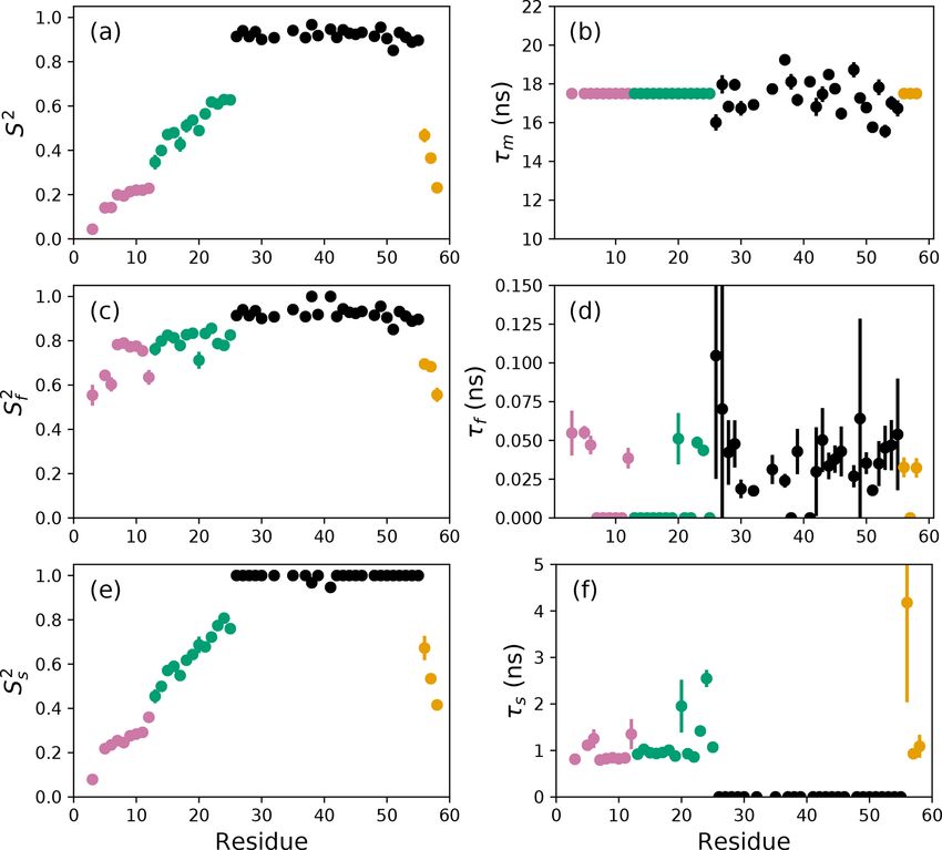
252                                                T. Crawley and A. G. Palmer III: Bootstrap aggregation in model selection

model-free spectral density functions (Mandel et al., 1995;       and ωH are the 15 N and 1 H Larmor frequencies. Thus, the
Gill et al., 2016). The resulting χ 2 residual sum-of-squares     number of spectral density values N = 3G, in which G is the
variables are penalized for the number of adjustable param-       number of static magnetic fields utilized. In the present ap-
eters in each model function, the model with the lowest pe-       plication, G = 4. The set of experimental spectral densities
nalized residual sum-of-squares is selected as optimal, and       is described using the following notation:
the best-fit parameters of the model are reported. However,
this procedure is subject to model selection error: random        y = {yj } = {y1 , y2 , . . ., yN } ,                         (1)
statistical variation in the experimental data may lead to one
                                                                  in which the yj = J (ωj ) are ordered in increasing values of
model chosen as optimal for a given data set, but another
                                                                  ω. The values of J (0) are ordered additionally by increas-
model, with different set of parameters, may be selected if
                                                                  ing values of the static magnetic field. The experimental data
the experimental data were replicated, with consequent dif-
                                                                  sets utilized in the present work are not affected by chemical
ferent random variation. The problem of joint model selec-
                                                                  exchange contributions to spin relaxation, but such contribu-
tion and parameter estimation has been explored elegantly
                                                                  tions can be taken into account from the field dependence of
by d’Auvergne and Gooley (2007, 2008a, b) and by Abergel
                                                                  transverse relaxation rate constants prior to the model-free
et al. (2014).
                                                                  analysis (Kroenke et al., 1998).
   The present paper addresses model selection error by us-
                                                                      The extended model-free spectral density function used to
ing the approach of bootstrap aggregation or bagging. This
                                                                  fit 15 N spin relaxation data is given by the following:
concept originated from a desire to improve the performance
of machine learning algorithms. Thus, Breiman showed that                   2 Sf2 Ss2 τm         Sf2 (1 − Ss2 )τ1

predictor accuracy and stability improved when averaging          J (ω) =                    +
                                                                            5 (1 + ω2 τm2 )        (1 + ω2 τ12 )
predictor values obtained from bootstrap replicates of the
                                                                                    (1 − Sf2 )Ss2 τ2 (1 − Sf2 )(1 − Ss2 )τ3

original training set (Breiman, 1996). Buja and Stuetzle sub-
                                                                                 +                    +                       , (2)
sequently extended the use of bagging to generalized sta-                            (1 + ω2 τ22 )           (1 + ω2 τ32 )
tistical analysis and showed sampling with and without re-
placement yield equivalent improvements (Buja and Stuet-          in which τ1−1 = τm−1 + τs−1 , τ2−1 = τm−1 + τf−1 , τ3−1 = τm−1 +
zle, 2006). The approach and notation of Efron are used in        τs−1 +τf−1 , and τf < τs . The set of possible model parameters
the following (Efron, 2014).                                      in this function are given by the following:
   Bootstrap aggregation improves parameter stability; con-
sequently, the resulting variations in model-free parameter       µ = {µk } = {τm , Sf2 , Ss2 , τf , τs } ,                    (3)
values, for example between atomic sites or functional states
in a given macromolecule, are more likely to be biologi-          in which τm is the (effective) overall rotational correlation
cally or chemically meaningful. Although applicable to most       time, Sf2 is the square of the generalized order parameter
model selection situations, bootstrap aggregation exhibits the    for internal motions on a fast (τf ≤ 150 ps) timescale, and Ss2
most pronounced benefits when the data justify two distinct       is the square of the generalized order parameter for internal
models with similar degrees of certainty.                         motions on a slow (τs > 150 ps) timescale (vide infra). The
   Bootstrap aggregation for model-free analysis of NMR           square of the generalized order parameter S 2 = Sf2 Ss2 . Over-
spin relaxation rate constants is illustrated by application      all rotational diffusion has been assumed to be isotropic for
to backbone amide 15 N spin relaxation data that have been        simplicity; this assumption can be relaxed as needed (Lee
recorded at 1 H magnetic fields of 600, 700, 800, and             et al., 1997). The spectral density data are fit with a set of
900 MHz for the bZip domain of the S. cerevisiae transcrip-       nested models. The full model, Model 5, contains all five pa-
tion factor GCN4 by Gill and coworkers (Gill et al., 2016).       rameters, while simpler models, Models 1–4, are generated
                                                                  by fixing the value of one or more parameters, effectively
                                                                  removing such parameters from the model. Thus,
2   Theory                                                              Model 1: µ = {τm , Sf2 , 1, 0, 0}

In the following, the notation used by Efron is rephrased               Model 2: µ = {τm , Sf2 , 1, τf , 0}
in terms appropriate for NMR spin relaxation data (Efron,
                                                                        Model 3: µ = {τm , 1, Ss2 , 0, τs }
2014). Laboratory-frame nuclear spin relaxation rate con-
stants for backbone 15 N spins can be transformed into sets             Model 4: µ = {τm , Sf2 , Ss2 , 0, τs }
of spectral density function values, J (ω), in which ω is an
eigenfrequency of the spin system (Farrow et al., 1995; Gill            Model 5: µ = {τm , Sf2 , Ss2 , τf , τs }.
et al., 2016). Laboratory-frame 15 N relaxation rate constants,   The optimal model t1 and associated parameter values µ are
typically R1 , R2 , and the steady-state nuclear Overhauser en-   obtained as follows:
hancement (NOE), recorded at a single static magnetic field
yield estimates of J (0), J (ωN ), and J (0.87ωH ), in which ωN   µ̂ = {µ̂k } = t1 (y) ,                                       (4)

Magn. Reson., 2, 251–264, 2021                                                              https://doi.org/10.5194/mr-2-251-2021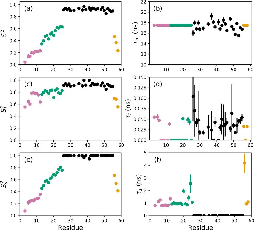
T. Crawley and A. G. Palmer III: Bootstrap aggregation in model selection                                                          253

using the lowest penalized residual sum-of-squares as de-                To make the above formalism concrete, suppose that for
scribed above. In the present work, the small-sample AICC           a given set of spectral density values, model selection and
criterion was used for model selection (Hurvich and Tsai,           parameter optimization for B bootstrap samples yields B2
1989).                                                              samples in which Model 2 is optimal and B3 samples in
   In general, a non-parametric bootstrap sample is generated       which Model 3 is optimal, with B = B2 + B3 . The bootstrap-
by draws with replacement from the original data y and de-          aggregated estimates of S̃f2 and τ̃f are given by the following:
fined as follows:                                                             "                #
                                                                       2     1 X 2∗ X
                   ∗
y ∗i = {yij∗ } = {yi1    ∗            ∗                             S̃f =           S̃ +      1 ,                               (11)
                      , yi2 , . . ., yiN },                  (5)            B i∈B fi     i∈B3
                                                                                  2
                                                                              "              #
in which i = 1, . . .B and B is the total number of bootstrap               1 X ∗ X
samples. The nature of spectral density data requires care in       τ̃f =         τ̃ +     0                                    (12)
                                                                           B i∈B fi i∈B
generating bootstrap samples, and the particular procedure                          2           3

employed in the present work is described in Sect. 3.               because Model 3 fixes Sf2 = 1 and τf = 0. As another exam-
   A conventional non-parametric bootstrap determination of         ple, suppose that for a given set of spectral density values,
the standard deviations of the parameters µ̂ begins by de-          model selection and parameter optimization for B bootstrap
termining fitted parameters for the ith bootstrap sample as         samples yields B4 samples in which Model 4 is optimal and
follows:                                                            B5 samples in which model 5 is optimal, with B = B4 + B5 .
                                                                    The bootstrap-aggregated estimates of S̃f2 and τ̃f are given by
µ̂∗i = {µ̂∗ik } = t1 (y ∗i ) ,                               (6)
                                                                    the following:
in which the fitting model is fixed to the optimal model se-              1X B
lected in fitting the original spectral density values, and only    S̃f2 =     S̃ 2∗ ,                                             (13)
model parameter values are optimized. The bootstrap esti-                 B i=1 fi
                                                                            "                   #
mate of the standard deviation for the kth parameter is de-               1 X          X
                                                                      2                      2∗
rived from the following expressions:                               τ̃f =         0+       τ̃fi                                    (14)
                                                                          B i∈B        i∈B
                                                                                     4         5
           B
       1X                                                           because both Models 4 and 5 fit Sf2 as a parameter, but Model
µ̂∗k =       µ̂∗ ,                                           (7)
       B i=1 ik                                                     4 fixes τf = 0.
       "
                B
                               #1/2                                    A smoothed standard deviation for µ̃ can be obtained us-
  ∗        1 X        ∗    ∗ 2                                      ing the plug-in principle (Efron, 2014). Here, the cumulative
σ̂k =              (µ̂ − µ̂k )      .                        (8)
         B − 1 i=1 ik                                               distribution functions for the parameters of interest are esti-
                                                                    mated using the empirical distribution function of the boot-
In the conventional approach, the reported results of the data      strap replicates. Using the above notation, the number of
analysis are {µ̂k } and {σ̂k∗ }. Model selection error is not as-   times that the ith bootstrap replicate, y ∗i , contains the spectral
sessed. This form of bootstrap simulation is an alternative to      density value yj is given by the following:
Monte Carlo simulations to determine parameter uncertain-
ties, which could be regarded as parametric bootstrap simu-         Yij∗ = #{yik
                                                                              ∗
                                                                                 = yj } .                                          (15)
lations (vide infra).                                               With this definition, Y ∗i is a vector enumerating the represen-
   In contrast to the conventional procedure, bootstrap aggre-      tation of each original data point in the ith bootstrap replicate
gation determines both the optimal fitted model and associ-         as follows:
ated model parameters for each bootstrap sample. Thus, the
optimal model ti is determined for the ith bootstrap sample         Y ∗i = {Yi1
                                                                              ∗     ∗
                                                                                , Yi2            ∗
                                                                                      , . . ., YiN }.                              (16)
using the same model selection strategy as for the original         Further, the average representation of the original spectral
data as follows:                                                    density value yj across the B bootstrap replicates is given by
                                                                    the following:
µ̃∗i = {µ̃∗ik } = ti (y ∗i ) .                               (9)
                                                                                B
                                                                      ∗      1X
Unlike the conventional bootstrap procedure, the different          Yj =          Y∗ .                                             (17)
members of the set µ̃∗i obtained by bootstrap aggregation rep-               B i=1 ij
resent different models as well as different sets of optimized      The covariance between the representation of the j th spectral
parameters. The aggregated, or smoothed, estimator of the           density value and the kth model-free parameter value across
kth model parameter is given by the following:                      B bootstrap replicates is given by the following:
           B                                                                      B
        1X                                                                     1X             ∗

             µ̃∗ .                                                                   Yij∗ − Y j µ̃∗ik − µ̃k .

µ̃k =                                                       (10)    cov
                                                                     ˆ jk =                                                        (18)
        B i=1 ik                                                               B i=1

https://doi.org/10.5194/mr-2-251-2021                                                                   Magn. Reson., 2, 251–264, 2021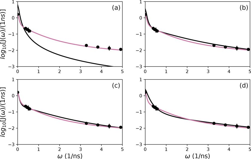
254                                                 T. Crawley and A. G. Palmer III: Bootstrap aggregation in model selection

Finally, the smoothed estimate of the standard deviation for       Table 1. Bootstrap selections.
the kth model-free parameter is calculated from the following
expression:                                                             i        pij        Yij∗      i      pij         Yij∗
      "                #1/2                                             1     [1,2,3,4]   [1,1,1,1]   11   [4,2,3,4]   [0,1,1,2]
            N
        1 X
σ̃k =           ˆ 2j k
               cov          .                            (19)           2     [1,1,3,4]   [2,0,1,1]   12   [1,4,3,4]   [1,0,1,2]
        N j =1                                                          3     [1,2,1,4]   [2,1,0,1]   13   [1,2,4,4]   [1,1,0,2]
                                                                        4     [1,2,3,1]   [2,1,1,0]   14   [1,1,2,2]   [2,2,0,0]
   In bootstrap aggregation, the reported results consist of the        5     [2,2,3,4]   [0,2,1,1]   15   [1,1,3,3]   [2,0,2,0]
smoothed estimators {µ̃k } and {σ̃k } incorporating the effects         6     [1,2,2,4]   [1,2,0,1]   16   [1,1,4,4]   [2,0,0,2]
of model selection uncertainty. As noted by Efron, σ̃k ≤ σ̂ku ,         7     [1,2,3,2]   [1,2,1,0]   17   [2,2,3,3]   [0,2,2,0]
in which σ̂ku is obtained using Eq. (8) naively applied to the          8     [3,2,3,4]   [0,1,2,1]   18   [2,2,4,4]   [0,2,0,2]
bootstrap-aggregated data (rather than to data analyzed with            9     [1,3,3,4]   [1,0,2,1]   19   [3,3,4,4]   [0,0,2,2]
                                                                        10    [1,2,3,3]   [1,1,2,0]
a fixed model as above) (Efron, 2014).

3   Methods
                                                                   bootstrap sample could be generated in which one particular
Backbone amide 15 N spin relaxation data have been reported        J (0) value is represented exclusively.
at G = 4 1 H static magnetic fields of 600, 700, 800, and              To avoid such highly unrepresentative possibilities, boot-
900 MHz for the bZip domain of the S. cerevisiae transcrip-        strap samples were generated by enumerating the 193 =
tion factor GCN4 by Gill and coworkers (Gill et al., 2016).        6859 possible arrangements in which at most two spectral
Experimental values of R1 , R2 , and the steady-state NOE          density values from each set of J (0), J (ωN ), and J (0.87ωH )
measured at each magnetic field for each residue were con-         are duplicated. The 19 possible arrangements of the G = 4
verted to spectral density values using the following expres-      indices {1, 2, 3, 4} and corresponding Yij for selecting boot-
sions (Farrow et al., 1995; Gill et al., 2016):                    strap samples of J (0), J (ωN ), and J (0.87ωH ) are shown in
                                                                   Table 1. In this table, pij is a pointer vector selecting data
                4                                                  from a particular set of spectral density values. For exam-
J (0.87ωH ) =       σNH                                    (20)
                 2
              5dNH                                                 ple p4j = [1, 2, 3, 1]; applying this pointer to the set of J (0)
          4(R1 − 1.249σNH )                                        values would select the J (0) values obtained at 600 (×2),
J (ωN ) =                                                  (21)    700, and 800 MHz. The corresponding counter vector Y4j      ∗ =
               2 + 4c2
            3dNH      NH                                           [2, 1, 1, 0] is the numbers of times J (0) values recorded at the
        6(R2 − 0.5R1 − 0.454σNH )                                  different fields were sampled. The process would be repeated
J (0) =           2 + 4c2
                                  ,                        (22)
              3dNH      NH                                         for the other sets of spectral density values. For example, the
                                                                   i = 1260th bootstrap sample uses p4j to select J (0), p10j to
in which σNH = (NOE − 1)R1 γN γH−1 , cNH = 3−1/2 1σ ωN ,           select J (ωN ), and p6j to select J (0.87ωH ). The full vector
                         −3
dNH = (µ0 /4π ) γH γN rNH   , rNH = 0.102 nm is the N–H bond       Y ∗i of length N = 12 is obtained by concatenating the indi-
length, and 1σ = −172 ppm is the 15 N chemical shift               vidual Y4j ∗ , Y ∗ , and Y ∗ vectors from the table. With this
                                                                                    10j      6j
anisotropy. A single value of J (0) was obtained for each          procedure, the first bootstrap sample is identical to the origi-
residue as the weighted mean (using propagated experimen-          nal data. The mean and uncertainty were determined for J (0)
tal uncertainties) of the values obtained from the G static        for each bootstrap sample as described above for the original
magnetic fields. The uncertainty in the mean J (0) was ob-         data so that fitting of bootstrap samples was performed in the
tained by jackknife simulations. For each residue, the spec-       same fashion as for the original data.
tral density values used for model fitting consist of the mean         The data were analyzed using three procedures. First, a
J (0), G values of J (ωN ), and G values of J (0.87ωH ), for a     conventional analysis, Eq. (4), was performed in which opti-
total of nine data points.                                         mal models t1 and model parameters {µ̂k } were determined
   As noted above, the 15 N spectral density values for each       for each amino acid residue (for which data were available)
backbone amide consist of G = 4 values of each of J (0),           using AICC . The uncertainties in model parameters, denoted
J (ωN ), and J (0.87ωH ). Random sampling with replacement         {σ̂k }, were determined by 500 Monte Carlo simulations us-
from the N = 12 values to generate bootstrap samples, as           ing the measured experimental uncertainties in the spectral
normally applied, could result in samples in which the rela-       density values (Gill et al., 2016). Second, the optimal model
tive numbers of spectral density values from each class are        was determined as in the first procedure, but the uncertainties
highly skewed. For example, a bootstrap sample could be            in model parameters, {σ̂k∗ }, were determined by the conven-
generated without any J (0) values, leading to very anoma-         tional bootstrap, using Eq. (8). In both of these approaches,
lous fitted parameters. At the other extreme, random sam-          error estimates were obtained while fixing the model for each
pling with replacement could result in samples in which            Monte Carlo or bootstrap sample as the optimal model t1 se-
a single value was highly overrepresented. For example, a          lected against the original data. Third, the smoothed model

Magn. Reson., 2, 251–264, 2021                                                            https://doi.org/10.5194/mr-2-251-2021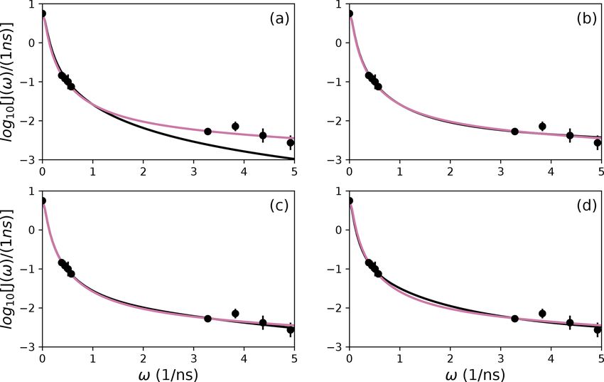
T. Crawley and A. G. Palmer III: Bootstrap aggregation in model selection                                                            255

                                                                         original analysis of the relaxation data (Gill et al., 2016). Lo-
                                                                         cal values of τm can be used to determine the overall rota-
                                                                         tional correlation time or diffusion tensor using established
                                                                         methods (Lee et al., 1997). Alternatively, the fitting process
                                                                         could be modified to globally optimize the overall rotational
                                                                         correlation time or diffusion tensor while independently op-
                                                                         timizing generalized order parameters and correlation times
                                                                         for individual residues (Mandel et al., 1995). In this scenario,
                                                                         bootstrap aggregation for the internal dynamical parameters
                                                                         would be performed by the same approach as used herein.

                                                                         4   Results

                                                                         The results of the conventional analysis using AICC for
                                                                         model selection and Monte Carlo error estimation are shown
                                                                         in Fig. 2. Each of the Monte Carlo simulations was analyzed
                                                                         using the optimal model determined from the original data.
                                                                         The optimal parameters differ slightly from those reported by
                                                                         Gill and coworkers because the present approach used a dif-
                                                                         ferent spectral density function and model selection method
                                                                         compared to the earlier work (Gill et al., 2016). The results
                                                                         of the conventional analysis using AICC for model selection
                                                                         and bootstrap resampling for error estimation are shown in
                                                                         Fig. 3. Each of the bootstrap data sets was analyzed using the
                                                                         optimal model determined from the original data. The results
                                                                         for bootstrap aggregation using AICC to determine the op-
                                                                         timal model for each bootstrap sample are shown in Fig. 4.
Figure 1. Flow chart for bootstrap aggregation for the model-free        The bootstrap-aggregated smoothed model-free parameters
formalism. Indices l, m, and n are determined for each bootstrap         were calculated using Eq. (10), and the smoothed parameter
sample from the index i using modulo arithmetic, in which // rep-        uncertainties were calculated using Eq. (19).
resents floor division, and % is the modulo (remainder) operation.          Bootstrap simulations in which a single optimal model is
The three indices l, m, and n select pointer and counter vectors from    utilized provide an alternative to Monte Carlo simulations for
Table 1. The three pointer vectors are used to generate bootstrap
                                                                         estimation of (unsmoothed) parameter uncertainties. The un-
samples for J (0), J (ωN ), and J (ωH ). The three counter vectors are
concatenated to form Y ∗i .
                                                                         certainties in σ̂ (S 2 ) obtained from Monte Carlo simulations
                                                                         and σ̂ ∗ (S 2 ) obtained from conventional bootstrap simula-
                                                                         tions are compared in Fig. 5a. The uncertainties have approx-
                                                                         imately the same range but are uncorrelated with each other.
parameters {µ̃k } and uncertainties {σ̃k } were determined by            These results suggest the non-parametric bootstrap samples
bootstrap aggregation using Eqs. (10) and (19), respectively.            simulate the actual data distribution in comparable manner
In this approach, the optimal model and parameters were de-              as the parametric Monte Carlo simulations but without as-
termined individually for each bootstrap sample as in Eq. (9).           suming a normal distribution of spectral density values. The
A flowchart outlining the process of performing bootstrap                smoothed parameter uncertainty obtained from Eq. (19) is
aggregation is shown in Fig. 1. Both Models 2 and 3 con-                 compared to the uncertainties from Monte Carlo simulations
tain a single generalized order parameter and a single inter-            in Fig. 5b. The increase in σ̃ (S 2 ) compared to σ̂ (S 2 ) re-
nal effective correlation time. The model selection strategy             flects the effect of model selection uncertainty. As noted by
employed herein assigns Model 2 if the internal correlation              Efron, the estimate of smoothed parameter uncertainty ob-
is < 0.15 ns and Model 3 if the internal correlation time is             tained from Eq. (19) is smaller than the naive estimate ob-
≥ 0.15 ns (vide infra).                                                  tained by applying Eq. (8) to the aggregated bootstrap sam-
   Values of a local τm were optimized for each residue in the           ples (Efron, 2014). To illustrate the advantage of Eq. (19),
well-ordered coiled-coil domain of the protein (residues 26–             Fig. 5c compares σ̂ u (S 2 ) obtained from Eq. (8) and σ̃ (S 2 )
55). Values of τm for residues in the basic region (residues 3–          obtained from Eq. (19). Similar trends are observed for other
25) and disordered C-terminus (residues 56–58) were fixed                model-free parameters (not shown).
at 17.5 ns, the average value obtained for ordered residues.                The performance of the conventional analysis, in which a
A similar approach was used by Gill and coworkers in the                 single optimal model is chosen, and bootstrap aggregation,

https://doi.org/10.5194/mr-2-251-2021                                                               Magn. Reson., 2, 251–264, 2021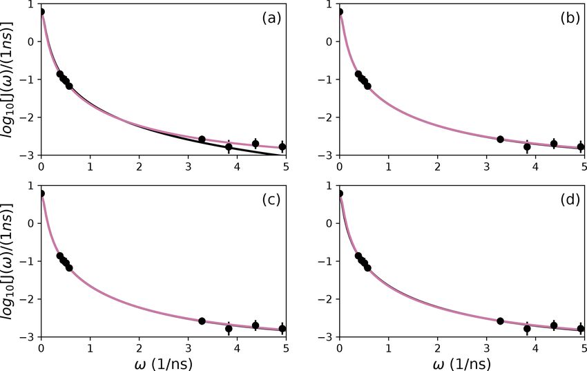
256                                                            T. Crawley and A. G. Palmer III: Bootstrap aggregation in model selection

Figure 2. Model-free parameters from conventional model selection using AICC and 500 Monte Carlo simulations to determine parameter
uncertainties. Values of S 2 , τm , Sf2 , τf , Ss2 , and τs are plotted vs. residue number. Overall correlation times (τm ) were determined individually
for residues in the coiled-coil region (black), while τm was fixed at 17.5 ns for residues in the basic region and C-terminus. Regions of the
protein are colored as basic region 1 (residues 3–12) (reddish-purple), basic region 2 (residues 13–25) (green), coiled-coil (residues 26–55)
(black), and disordered C-terminus (residues 56–58) (orange) (Gill et al., 2016).

Table 2. Model selection for selected residues.

                                  Residue       Fit         Model 1         Model 2        Model 3        Model 4        Model 5
                                  Arg 11        AICC             67.9            NA             57.2           33.3           34.2
                                                Boot            0.000          0.000           0.000          0.243          0.757
                                  Arg 26        AICC             39.2           23.4             NA            33.5           56.6
                                                Boot            0.000          0.566           0.316          0.096          0.022
                                  Asp 32        AICC             18.4           10.3             NA            22.3           46.2
                                                Boot            0.000          0.970           0.000          0.019          0.011
                                For each residue, the top line lists the AICC values determined by fitting the original data to Models
                                1–5. The second line enumerates the percentage of bootstrap samples for which the indicated model
                                exhibited the lowest AICC . Both Models 2 and 3 contain a single internal effective correlation time.
                                Model 2 is assigned if this correlation time is < 0.15 ns (and Model 3 is not assigned, NA). Model 3 is
                                assigned if this correlation time is ≥ 0.15 ns (and Model 2 is not assigned, NA).

in which parameter values are smoothed over all models, are                            original spectral density data and the smoothed model-free
illustrated for particular residues Arg 11, Arg 26, and Asp 32.                        parameters obtained by bootstrap aggregation. The optimal
Table 2 shows the values of AICC for each model fit to the                             single model selected by AICC is highlighted with an aster-
original spectral density and the percentage that each model                           isk.
was chosen in the bootstrap aggregation. Table 3 shows the                                To further illustrate bootstrap aggregation for Arg 11,
optimized model-free parameters for each model fit to the                              Arg 26, and Asp 32, Figs. 6, 7, and 8 show the distributions

Magn. Reson., 2, 251–264, 2021                                                                                      https://doi.org/10.5194/mr-2-251-2021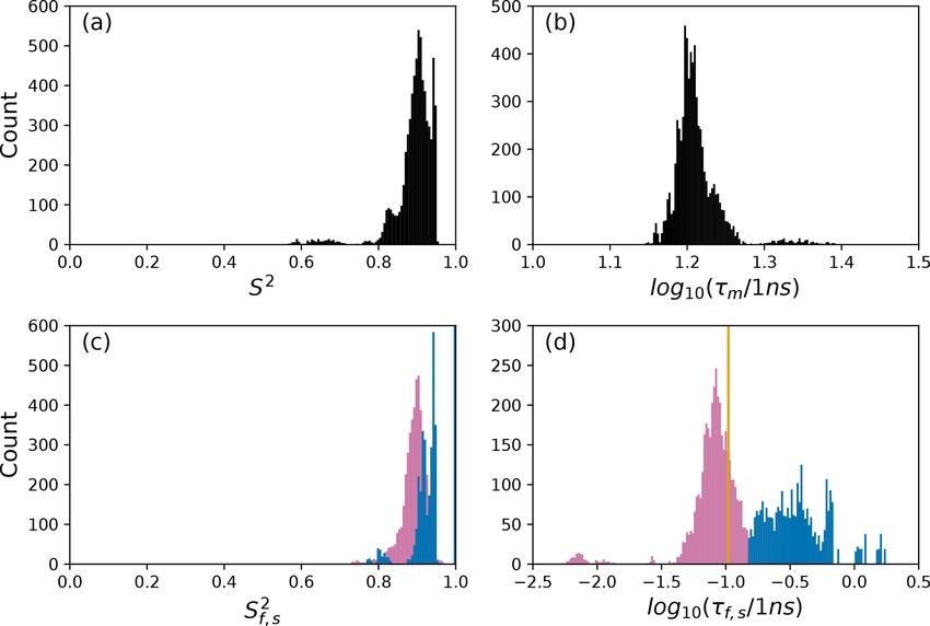
T. Crawley and A. G. Palmer III: Bootstrap aggregation in model selection 257
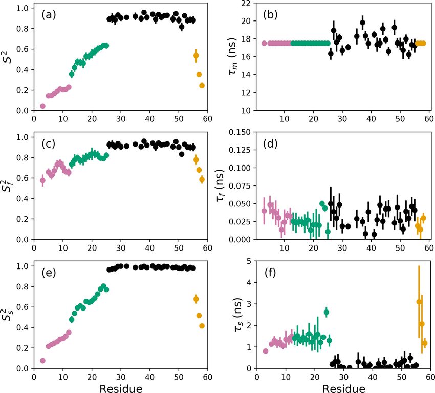
Figure 3. Model-free parameters from conventional model selection using AICC and bootstrap resampling to determine parameter uncer-
tainties. Values of S 2 , τm , Sf2 , τf , Ss2 , and τs are plotted vs. residue number. Parameter values are identical as in Fig. 2, but the uncertainty
estimates differ. Regions of the protein are colored as basic region 1 (residues 3–12) (reddish-purple), basic region 2 (residues 13–25) (green),
coiled-coil (residues 26–55) (black), and disordered C-terminus (residues 56–58) (orange) (Gill et al., 2016).
Table 3. Model-free parameters for selected residues.
Residue Model τm S2 Sf2 Ss2 τf τs
Arg 11 1 17.5(fixed) 0.886 ± 0.015 0.886 ± 0.015 1 0 0
3 17.5(fixed) 0.480 ± 0.006 1 0.480 ± 0.006 0 0.761 ± 0.011
4∗ 17.5(fixed) 0.220 ± 0.017 0.754 ± 0.015 0.292 ± 0.018 0 0.838 ± 0.014
5 17.5(fixed) 0.211 ± 0.017 0.646 ± 0.022 0.326 ± 0.020 0.036 ± 0.004 1.13 ± 0.09
Smooth 17.5(fixed) 0.208 ± 0.005 0.662 ± 0.029 0.316 ± 0.013 0.033 ± 0.006 1.31 ± 0.21
Arg 26 1 14.55 ± 0.48 0.954 ± 0.031 0.954 ± 0.031 1 0 0
2∗ 16.01 ± 0.55 0.914 ± 0.024 0.914 ± 0.024 1 0.105 ± 0.054 0
4 16.00 ± 0.73 0.878 ± 0.038 0.935 ± 0.037 0.939 ± 0.013 0 0.274 ± 0.165
5 17.28 ± 2.69 0.812 ± 0.103 0.871 ± 0.070 0.932 ± 0.057 0.030 ± 0.020 0.93 ± 1.15
Smooth 16.33 ± 0.68 0.891 ± 0.027 0.925 ± 0.037 0.972 ± 0.015 0.050 ± 0.024 0.19 ± 0.14
Asp 32 1 16.28 ± 0.39 0.944 ± 0.022 0.944 ± 0.022 1 0 0
2∗ 16.92 ± 0.46 0.908 ± 0.025 0.908 ± 0.025 1 0.017 ± 0.016 0
4 16.92 ± 1.31 0.908 ± 0.053 1.000 ± 0.060 0.908 ± 0.040 0 0.02 ± 0.48
5 19.58 ± 3.45 0.756 ± 0.138 0.853 ± 0.074 0.887 ± 0.091 0.010 ± 0.009 8.33 ± 3.18
Smooth 17.06 ± 0.34 0.909 ± 0.017 0.911 ± 0.015 0.998 ± 0.005 0.018 ± 0.004 0.035 ± 0.074
For each residue, parameter values for Models 1–5 are calculated from the fit of the original data to the relevant spectral density function, with errors determined
by Monte Carlo simulation. The model selected by AICC is indicated by ∗ . Smooth values are obtained by averaging the best fit parameter values across bootstrap
samples as in Eq. (10), with errors determined as indicated in Eqs. (15)–(19).
https://doi.org/10.5194/mr-2-251-2021 Magn. Reson., 2, 251–264, 2021258 T. Crawley and A. G. Palmer III: Bootstrap aggregation in model selection
Figure 4. Smoothed model-free parameters from bootstrap aggregation to determined smoothed parameter estimates and uncertainties.
Values of S 2 , τm , Sf2 , τf , Ss2 , and τs are plotted vs. residue number. Regions of the protein are colored as basic region 1 (residues 3–12)
(reddish-purple), basic region 2 (residues 13–25) (green), coiled-coil (residues 26–55) (black), and disordered C-terminus (residues 56–58)
(orange) (Gill et al., 2016).
Figure 5. Comparison of model-free parameter uncertainties. (a) Uncertainties for S 2 calculated from Monte Carlo, σ̂k , and bootstrap
simulations, σ̂k∗ , for a single optimal model. (b) Uncertainties for S 2 calculated from Monte Carlo simulations for a single optimal model and
smoothed σ̃k calculated from bootstrap aggregation. (c) Uncertainties σ̂ku and σ̃ for S 2 calculated from bootstrap aggregation, illustrating the
smaller variability obtained using Eq. (19) for calculation of parameter sample deviations.
of model-free parameters determined from the optimal model 5 Discussion
for each bootstrap sample. The calculated spectral density
function for bootstrap aggregation is compared to the fit- The difficulties posed by conventional model selection strate-
ted spectral density functions for each model in Figs. 9, 10, gies, in which a single optimal model is chosen using AICC
and 11. or other fitness statistic, are illustrated for the bZip domain
of GCN4 in Fig. 2. In particular, some residues in the ba-
sic region (residues 3–25) are analyzed using Model 4, in
which τf = 0 and other residues are analyzed with Model 5,
Magn. Reson., 2, 251–264, 2021 https://doi.org/10.5194/mr-2-251-2021T. Crawley and A. G. Palmer III: Bootstrap aggregation in model selection 259
aggregation. The original optimization against the measured
data yielded AICC values of 33.3 for Model 4 and 34.1 for
Model 5. The conventional analysis then selects Model 4
(with τf = 0) as optimal, even though AICC for Model 5 is
only slightly larger. In contrast the bootstrap analysis sug-
gests that Model 4 would be optimal for 24 % and Model
5 would be optimal for 76 % of randomly chosen data, un-
der the assumption that the bootstrap samples represent the
underlying distribution of spectral density values. Bootstrap
smoothing then averages each model-free parameter over the
empirical distributions shown in Fig. 6, with resulting opti-
mized spectral density curves compared to the original exper-
imental data in Fig. 9. The results for Model 4 in Table 3 and
the corresponding vertical orange line in Fig. 9 show that the
selection of Model 4 in the conventional analysis results in
an estimate for τs that is skewed toward the lower boundary
of the τs bootstrap distribution.
The results shown for residue Arg 26 in Tables 2 and 3 and
Figs. 7 and 10 illustrate another advantage of bootstrap ag-
gregation. In this case, the original optimization against the
measured data yielded an AICC value of 23.4 for Model 2,
substantially smaller than for any other model, implying
a single model might be an adequate description for this
residue. However, the bootstrap distribution for the inter-
nal correlation times is bimodal. The conventional choice
of Model 2 results in an estimate of τf roughly centered in
the distribution, but the smoothed bootstrap estimates iden-
tify the presence of two separable timescales for internal mo-
tions, one with a mean of 0.052 ± 0.019 and the other with a
Figure 6. Distribution of model-free parameters from bootstrap ag- mean of 0.13 ± 0.08. Residue 26 is at the juncture between
gregation for residue Arg 11. Color coding is Sf2 or τf (reddish- the basic region and coiled-coil motif of the GCN4 bZip do-
purple) and Ss2 or τs (blue). The orange line in (c) indicates the value main; consequently, the latter effective internal correlation
of τs obtained for the optimal single (unsmoothed) model, Model 4. time might represent a vestige of the more pronounced mo-
For clarity, null values of 1 for generalized order parameters and 0
tions evident in the basic region. The critical value of 0.15 ns
for internal effective correlation times are not shown in the graphs;
used to separate fast from slow motions in the present work
τf = 0 is observed 1664 times.
was chosen empirically to distinguish the two distributions
observed for residue 26 (and used for all other residues).
More sophisticated clustering algorithms could be used to
in which τf > 0. The resulting values of the other model-free make this distinction between Models 2 and 3.
parameters are systematically affected depending on whether The results shown for residue Asp 32 in Tables 2 and 3
or not τf = 0. These systematic effects are evident most and Figs. 8 and 11 illustrate a case of strong agreement be-
clearly in the scatter in Sf2 and τs for residues in the basic tween the conventional analysis and bootstrap aggregation
region. The advantages of bootstrap aggregation in smooth- when a single motional model is strongly favored by the ex-
ing over variability in model selection is evident in Fig. 4, perimental data. The distributions shown in Fig. 8 then repre-
in which the residue-to-residue variability of the model-free sent the variability in model-free parameters across the boot-
parameters is reduced. Thus, the distributions of τf and τs strap samples. These results would be comparable to results
are much more uniform within the four regions of the pro- obtained in Fig. 3, in which the bootstrap samples were used
tein, suggesting rather uniform timescale processes in each to estimate model-free parameter uncertainties σ̂k∗ for a sin-
subdomain. The similarity in the distributions for σ̂ (S 2 ) and gle fixed optimal model.
σ̂ ∗ (S 2 ), shown in Fig. 5a, indicates that the bootstrap proce- The present application of bootstrap aggregation used spin
dure adequately samples the distribution of parameter values. relaxation data recorded at four static magnetic fields. A total
That is, the reduction in parameter variability from bootstrap of 6859 bootstrap samples were used to calculate smoothed
aggregation does not result from restricted sampling. parameter estimates. Data recorded at three static magnetic
The results shown for residue Arg 11 in Tables 2 and 3 fields provide nine spectral density values but allow only
and Figs. 6 and 9 illustrate the mechanics behind bootstrap 73 = 343 bootstrap samples. To test the effect of such a dras-
https://doi.org/10.5194/mr-2-251-2021 Magn. Reson., 2, 251–264, 2021260 T. Crawley and A. G. Palmer III: Bootstrap aggregation in model selection Figure 7. Distribution of model-free parameters from bootstrap aggregation for residue Arg 26. Color coding is Sf2 or τf (reddish-purple) and Ss2 or τs (blue). The orange line in (c) indicates the value of τf obtained for the optimal single (unsmoothed) model, Model 2. For clarity, null values of 1 for generalized order parameters and 0 for internal effective correlation times are not shown in the graphs; Sf2 = 1 is observed 2167 times, Ss2 = 1 is observed 3884 times, τf = 0 is observed 2823 times, and τs = 0 is observed 3884 times. Figure 8. Distribution of model-free parameters from bootstrap aggregation for residue Asp 32. Color coding is Sf2 or τf (reddish-purple) and Ss2 or τs (blue). The orange line in (c) indicates the value of τf obtained for the optimal single (unsmoothed) model, Model 2. For clarity, null values of 1 for generalized order parameters and 0 for internal effective correlation times are not shown in the graphs; Ss2 = 1 was observed 6650 times. tic reduction in the size of the bootstrap sample, the relax- are obtained for each residue, after averaging the three values ation rate constants recorded at 600, 800, and 900 MHz were of J (0). The smaller number of spectral density values results analyzed for the disordered basic region (residues 3–25). in smaller numbers of degrees of freedom when fitting the This preserves the same range of sampled frequencies as for model-free spectral density models. As a consequence, only the original analysis, but only seven spectral density values Models 3 and 4 were selected for the basic region in the con- Magn. Reson., 2, 251–264, 2021 https://doi.org/10.5194/mr-2-251-2021
T. Crawley and A. G. Palmer III: Bootstrap aggregation in model selection                                                              261

Figure 9. Comparison of individual fits for Arg 11 of (a) Model 1, (b) Model 3, (c) Model 4, and (d) Model 5 (black lines) or the bootstrap
aggregation smoothed fit (reddish-purple line) to (circles) experimental spectral density values.

Figure 10. Comparison of individual fits for Arg 26 of (a) Model 1, (b) Model 3, (c) Model 4, and (d) Model 5 (black lines) or the bootstrap
aggregation smoothed fit (reddish-purple line) to (circles) experimental spectral density values.

ventional analysis; essentially, the data were not sufficient to          to fully statistically characterize the information content of
determine τf and τs simultaneously (Model 5). Nonetheless,                such measurements within the extended model-free formal-
bootstrap aggregation was effective in smoothing the effects              ism.
of model selection error between Models 3 and 4, even with
only 343 bootstrap samples (not shown). A number of stud-                 6   Conclusions
ies have investigated the number of model parameters that
can be determined from backbone amide 15 N relaxation data                Model selection error is a classical problem in statistics and
recorded at high static magnetic fields (Khan et al., 2015; Gill          has been recognized as a concern in the model-free analysis
et al., 2016; Abyzov et al., 2016). The present results suggest           of NMR spin relaxation data since the work of d’Auvergne
that measurements at four static magnetic fields are required             and Gooley (2007, 2008a, b). Bootstrap aggregation has

https://doi.org/10.5194/mr-2-251-2021                                                                Magn. Reson., 2, 251–264, 2021
262                                                    T. Crawley and A. G. Palmer III: Bootstrap aggregation in model selection

Figure 11. Comparison of individual fits for Asp 32 of (a) Model 1, (b) Model 3, (c) Model 4, and (d) Model 5 (black lines) or the bootstrap
aggregation smoothed fit (reddish-purple line) to (circles) experimental spectral density values.

emerged as a powerful approach for incorporating selection                surements at multiple static magnetic fields, promises to ad-
error into statistical model-building (Buja and Stuetzle, 2006;           vance efforts to understand the interplay between conforma-
Efron, 2014). However, bootstrap aggregation requires suf-                tion and function in biology.
ficient numbers of data points to allow faithful resampling
of the distribution of the data. This issue is made more se-
rious by the nature of nuclear spin relaxation data: spec-                Code and data availability. A Jupyter notebook (Python 3.6) is
tral density values for J (0), J (ωN ), and J (0.87ωH ) are very          provided for performing all data analyses reported in the publica-
different and should not be interchanged by resampling. As                tion. The NMR data analyzed in the publication are available at
shown in the present work, resampling within blocks of spec-              Mendeley Data (https://doi.org/10.17632/vpwz6mrynr.1; Gill et al.,
                                                                          2021).
tral density values clustered as J (0), J (ωN ), and J (0.87ωH )
recorded at three or four static magnetic fields is sufficient
to enable bootstrap aggregation. However, the larger data set
                                                                          Supplement. The supplement related to this article is available
available from four static magnetic fields allows more reli-              online at: https://doi.org/10.5194/mr-2-251-2021-supplement.
able resolution of two internal correlation times, τf < 0.15 ns
and τs ≥ 0.15 ns.
   Aggregation improves parameter stability by averaging                  Author contributions. AGP conceived the project. Calculations
over all models represented in the bootstrap sample. As                   and writing of the paper were performed by TC and AGP.
applied to 15 N spin relaxation data for the bZip domain
of GCN4, bootstrap aggregation reduces residue-to-residue
variations in optimal model-free parameters, particularly in              Competing interests. The authors declare that they have no con-
the partially disordered basic region. Consequently, trends               flict of interest.
in the conformational dynamics along the polypeptide back-
bone that reflect actual physical properties of the protein be-
come more evident. Notably, local maxima in generalized                   Special issue statement. This article is part of the special issue
order parameters within the basic region (residues 3–25),                 “Geoffrey Bodenhausen Festschrift”. It is not associated with a con-
most evident for residues 8 and 9 and for residues 14 and                 ference.
15 in Fig. 4, reflect transient populations of helical confor-
mations observed in molecular dynamics simulations (Ro-
bustelli et al., 2013). NMR spin relaxation spectroscopy is               Acknowledgements. Arthur G. Palmer III acknowledges the
a powerful approach for interrogating conformational dy-                  support from the National Institutes of Health. Some of the work
                                                                          presented here was conducted at the Center on Macromolecular Dy-
namics of biological macromolecules. Bootstrap aggrega-
                                                                          namics by NMR Spectroscopy located at the New York Structural
tion, coupled with experimental NMR spin relaxation mea-

Magn. Reson., 2, 251–264, 2021                                                                      https://doi.org/10.5194/mr-2-251-2021
T. Crawley and A. G. Palmer III: Bootstrap aggregation in model selection 263
Biology Center, supported by the NIH National Institute of General Farrow, N., Zhang, O., Szabo, A., Torchia, D., and Kay, L.: Spectral
Medical Sciences. Arthur G. Palmer III is a member of the New density function mapping using 15 N relaxation data exclusively,
York Structural Biology Center. This paper is dedicated to Prof. Ge- J. Biomol. NMR, 6, 153–162, 1995.
offrey Bodenhausen on the occasion of his 70th birthday. Gill, M. L., Byrd, R. A., and Palmer, A. G.: Dynamics of GCN4
facilitate DNA interaction: a model-free analysis of an intrinsi-
cally disordered region, Phys. Chem. Chem. Phys., 18, 5839–
Financial support. This research has been supported by the 5849, 2016.
National Institutes of Health (grant nos. R35GM130398 and Gill, M. L., Byrd, R. A., and Palmer, A. G.: Data for: Dynamics
P41GM118302). of GCN4 facilitate DNA interaction: a model-free analysis of
an intrinsically disordered region, Mendeley Data [data set], V1,
https://doi.org/10.17632/vpwz6mrynr.1, 2021.
Review statement. This paper was edited by Malcolm Levitt and Halle, B. and Wennerström, H.: Interpretation of magnetic reso-
reviewed by three anonymous referees. nance data from water nuclei in heterogeneous systems, J. Chem.
Phys., 75, 1928–1943, 1981.
Hsu, A., Ferrage, F., and Palmer, A. G.: Analysis of NMR spin-
relaxation data using an inverse Gaussian distribution function,
References Biophys. J., 115, 2301–2309, 2018.
Hsu, A., Ferrage, F., and Palmer, A. G.: Correction: Analysis of
Abergel, D., Volpato, A., Coutant, E. P., and Polimeno, A.: On the NMR spin-relaxation data using an inverse Gaussian distribution
reliability of NMR relaxation data analyses: A Markov Chain function, Biophys. J., 119, 884–885, 2020.
Monte Carlo approach, J. Magn. Reson., 246, 94–103, 2014. Hurvich, C. M. and Tsai, C.-L.: Regression and time series model
Abyzov, A., Salvi, N., Schneider, R., Maurin, D., Ruigrok, R. W., selection in small samples, Biometrika, 76, 297–307, 1989.
Jensen, M. R., and Blackledge, M.: Identification of dynamic Khan, S. N., Charlier, C., Augustyniak, R., Salvi, N., Déjean, V.,
modes in an intrinsically disordered protein using temperature- Bodenhausen, G., Lequin, O., Pelupessy, P., and Ferrage, F.: Dis-
dependent NMR relaxation, J. Am. Chem. Soc., 138, 6240–6251, tribution of pico- and nanosecond motions in disordered proteins
2016. from nuclear spin relaxation, Biophys. J., 109, 988–999, 2015.
Box, G. E. P.: Science and statistics, J. Am. Stat. Assoc., 71, 791– Kroenke, C., Loria, J. P., Lee, L., Rance, M., and Palmer, A. G.:
799, 1976. Longitudinal and transverse 1 H-15 N dipolar/15 N chemical shift
Breiman, L.: Bagging predictors, Mach. Learn., 24, 123–140, 1996. anisotropy relaxation interference: unambiguous determination
Buja, A. and Stuetzle, W.: Observations on bagging, Stat. Sin., 16, of rotational diffusion tensors and chemical exchange effects in
323–351, 2006. biological macromolecules, J. Am. Chem. Soc., 120, 7905–7915,
Calandrini, V., Abergel, D., and Kneller, G. R.: Fractional protein 1998.
dynamics seen by nuclear magnetic resonance spectroscopy: Re- Lee, L., Rance, M., Chazin, W., and Palmer, A.: Rotational diffu-
lating molecular dynamics simulation and experiment, J. Chem. sion anisotropy of proteins from simultaneous analysis of 15 N
Phys., 133, 145101, https://doi.org/10.1063/1.3486195, 2010. and 13 Cα nuclear spin relaxation, J. Biomol. NMR, 9, 287–298,
Chen, J., Brooks C.L., 3rd, and Wright, P. E.: Model-free analysis 1997.
of protein dynamics: assessment of accuracy and model selection Lemaster, D. M.: Larmor frequency selective model free analysis of
protocols based on molecular dynamics simulation, J. Biomol. protein NMR relaxation, J. Biomol. NMR, 6, 366–374, 1995.
NMR, 29, 243–257, 2004. Lipari, G. and Szabo, A.: Model-free approach to the interpretation
Clore, G. M., Szabo, A., Bax, A., Kay, L. E., Driscoll, P. C., and of nuclear magnetic resonance relaxation in macromolecules. 1.
Gronenborn, A. M.: Deviations from the simple two-parameter Theory and range of validity, J. Am. Chem. Soc., 104, 4546–
model-free approach to the interpretation of nitrogen-15 nuclear 4559, 1982a.
magnetic relaxation of proteins, J. Am. Chem. Soc., 112, 4989– Lipari, G. and Szabo, A.: Model-free approach to the interpretation
4991, 1990. of nuclear magnetic resonance relaxation in macromolecules. 2.
d’Auvergne, E. J. and Gooley, P. R.: The use of model selection in Analysis of experimental results, J. Am. Chem. Soc., 104, 4559–
the model-free analysis of protein dynamics, J. Biomol. NMR, 4570, 1982b.
25, 25–39, 2003. Mandel, A. M., Akke, M., and Palmer, A. G.: Backbone dynamics
d’Auvergne, E. J. and Gooley, P. R.: Set theory formulation of of Escherichia coli ribonuclease HI: Correlations with structure
the model-free problem and the diffusion seeded model-free and function in an active enzyme, J. Mol. Biol., 246, 144–163,
paradigm, Mol. Biosyst., 3, 483–494, 2007. 1995.
d’Auvergne, E. J. and Gooley, P. R.: Optimisation of NMR dy- Mendelman, N. and Meirovitch, E.: SRLS analysis of 15 N–1 H
namic models I. Minimisation algorithms and their performance NMR relaxation from the protein S100A1: Dynamic structure,
within the model-free and Brownian rotational diffusion spaces, calcium binding, and related changes in conformational entropy,
J. Biomol. NMR, 40, 107–119, 2008a. J. Phys. Chem. B, 125, 805–816, 2021.
d’Auvergne, E. J. and Gooley, P. R.: Optimisation of NMR dynamic Mendelman, N., Zerbetto, M., Buck, M., and Meirovitch, E.: Con-
models II. A new methodology for the dual optimisation of the formational entropy from mobile bond vectors in proteins: A
model-free parameters and the Brownian rotational diffusion ten- viewpoint that unifies NMR relaxation theory and molecular dy-
sor, J. Biomol. NMR, 40, 121–133, 2008b. namics simulation approaches, J. Phys. Chem. B, 124, 9323–
Efron, B.: Estimation and accuracy after model selection, J. Am. 9334, 2020.
Stat. Assoc., 109, 991–1007, 2014.
https://doi.org/10.5194/mr-2-251-2021 Magn. Reson., 2, 251–264, 2021264 T. Crawley and A. G. Palmer III: Bootstrap aggregation in model selection Ollila, O. H. S., Heikkinen, H. A., and Iwaï, H.: Rotational dynam- Stone, M. J., Fairbrother, W. J., Palmer, A. G., Reizer, J., Saier, ics of proteins from spin relaxation times and molecular dynam- M. H., and Wright, P. E.: The backbone dynamics of the Bacil- ics simulations, J. Phys. Chem. B, 122, 6559–6569, 2018. lus subtilis glucose permease IIA domain determined from 15 N Palmer, A. G., Rance, M., and Wright, P. E.: Intramolecular motions NMR relaxation measurements, Biochemistry, 31, 4394–4406, of a zinc finger DNA-binding domain from xfin characterized 1992. by proton-detected natural abundance 13 C heteronuclear NMR Tugarinov, V., Liang, Z. C., Shapiro, Y. E., Freed, J. H., and spectroscopy, J. Am. Chem. Soc., 113, 4371–4380, 1991. Meirovitch, E.: A structural mode-coupling approach to 15 N Polimeno, A., Zerbetto, M., and Abergel, D.: Stochastic modeling NMR relaxation in proteins, J. Am. Chem. Soc., 123, 3055– of macromolecules in solution. I. Relaxation processes, J. Chem. 3063, 2001. Phys., 150, 184107, https://doi.org/10.1063/1.5077065, 2019a. Zerbetto, M., Anderson, R., Bouguet-Bonnet, S., Rech, M., Zhang, Polimeno, A., Zerbetto, M., and Abergel, D.: Stochastic modeling L., Meirovitch, E., Polimeno, A., and Buck, M.: Analysis of of macromolecules in solution. II. Spectral densities, J. Chem. 15 N–1 H NMR relaxation in proteins by a combined experimen- Phys., 150, 184108, https://doi.org/10.1063/1.5077066, 2019b. tal and molecular dynamics simulation approach: Picosecond- Robustelli, P., Trbovic, N., Friesner, R. A., and Palmer, A. G.: nanosecond dynamics of the Rho GTPase binding domain of Conformational dynamics of the partially disordered yeast tran- plexin-B1 in the dimeric state indicates allosteric pathways, J. scription factor GCN4, J. Chem. Theor. Comput., 9, 5190–5200, Phys. Chem. B, 117, 174–184, 2013. 2013. Smith, A. A., Ernst, M., Meier, B. H., and Ferrage, F.: Re- ducing bias in the analysis of solution-state NMR data with dynamics detectors, J. Chem. Phys., 151, 034102, https://doi.org/10.1063/1.5111081, 2019. Magn. Reson., 2, 251–264, 2021 https://doi.org/10.5194/mr-2-251-2021
You can also read