On the Oval Shapes of Beach Stones
←
→
Page content transcription
If your browser does not render page correctly, please read the page content below
On the Oval Shapes of Beach Stones
Theodore P. Hill
Abstract
arXiv:2008.04155v4 [cond-mat.soft] 4 Jul 2021
This article introduces a new geophysical theory, in the form of a single simple partial integro-
differential equation, to explain how frictional abrasion alone of a stone on a planar beach can
lead to the oval shapes observed empirically. The underlying idea in this theory is the intuitive
observation that the rate of ablation at a point on the surface of the stone is proportional to
the product of the curvature of the stone at that point and how often the stone is likely to be in
contact with the beach at that point. Specifically, key roles in this new model are played by both
the random wave process and the global (non-local) shape of the stone, i.e., its shape away from
the point of contact with the beach. The underlying physical mechanism for this process is the
conversion of energy from the wave process into potential energy of the stone. No closed-form or
even asymptotic solution is known for the basic equation, even in a 2-dimensional setting, but
basic numerical solutions are presented in both the deterministic continuous-time setting using
standard curve-shortening algorithms, and a stochastic discrete-time polyhedral-slicing setting
using Monte Carlo simulation.
Mathematics Subject Classification (2010). Primary 86A60, 53C44; Secondary 45K05, 35Q86
Key words and phrases. Curve shortening flow, partial integro-differential equation, support
function, Monte Carlo simulation, polyhedral approximation, frictional abrasion
1 Introduction
“The esthetic shapes of mature beach pebbles”, as geologists have remarked, “have an irresistible
fascination for sensitive mankind” [14]. This fascination dates back at least to Aristotle ([5]; see
[27]), and has often been discussed in the scientific literature (e.g., [6], [8], [10], [11], [16], [18], [24],
[28], [29], [35], [39], [40], and [41]).
Various mathematical models for the evolving shapes of 2- and 3-dimensional “stones”, both
purely mathematical models on curve-shortening flows and physical models under frictional abra-
sion, contain hypotheses guaranteeing that the shapes will become spherical in the limit (e.g., [2],
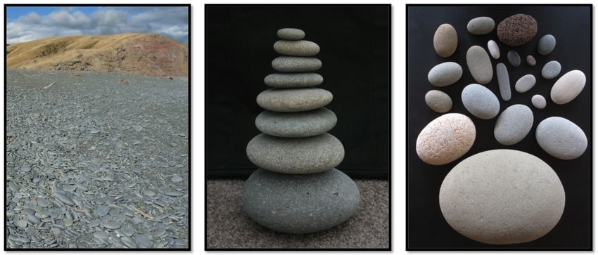
[4], [9], [20], and [21]). Observations of beach stones in nature, however, suggest that the “esthet-
ically fascinating” shapes of beach stones are almost never spherical. Instead, real beach stones
and artificial pebbles from laboratory experiments typically have elongated oval shapes (e.g., see
Figures 1 and 2). Furthermore, in his analysis of these oval shapes (see Figure 3) Black reported
that this “ovoid shape seems to be taken by all sorts of stones, from the soft sandstone to the hard
quartzite, and may therefore be independent of mineral composition, or relative hardness of the
stone” [8, p. 122].
The main goal of this paper is to introduce a simple mathematical equation based on physically
intuitive heuristics that may help explain the limiting (non-elliptical) oval shapes of stones wearing
down solely by frictional abrasion by waves on a flat sandy beach. Although very easy to state,
this new equation is technically challenging and no closed-form solution is known to the author for
most starting stone shapes or distributions of wave energies, even in a 2-d setting.
1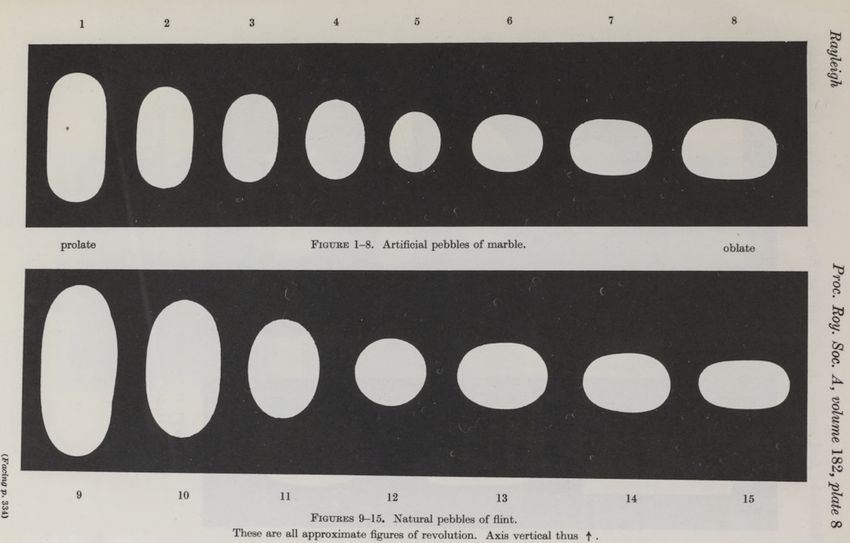
On the other hand, two different types of numerical approximations of solutions of this equa-
tion for various starting shapes indicate promising conformity with the classical experimental and
empirical shapes of beach stones found by Lord Rayleigh (son and biographer of Nobelist Lord
Rayleigh). One type of numerical solution of the equation models the evolving shapes of various
isolated beach stones in a deterministic continuous-time setting using standard techniques for solv-
ing curve-shortening problems, and the other type uses Monte Carlo simulation to approximate
typical changes in the stone shape in a discrete-time discrete-state setting.

Figure 1: Examples of artificial pebbles of marble (top row) abraded in his laboratory, and natural
pebbles of flint (bottom row) reported by Lord Rayleigh in 1944 [36].

Figure 2: Modern beach stones: stones on a beach in the Banks peninsula of New Zealand (left);
beach stones collected from a different beach on South Island by A. Berger (center); and beach
stones collected by the author on several continents (right; the largest is about 30 cm long, and
weighs about 13 kg).

Remark 1.1. As observed by Krynine, “on the seashore the similar pebbles are seen in the same
places” [27], and evidence of this is also apparent in Figure 2. Note that stones from the same

                                                 2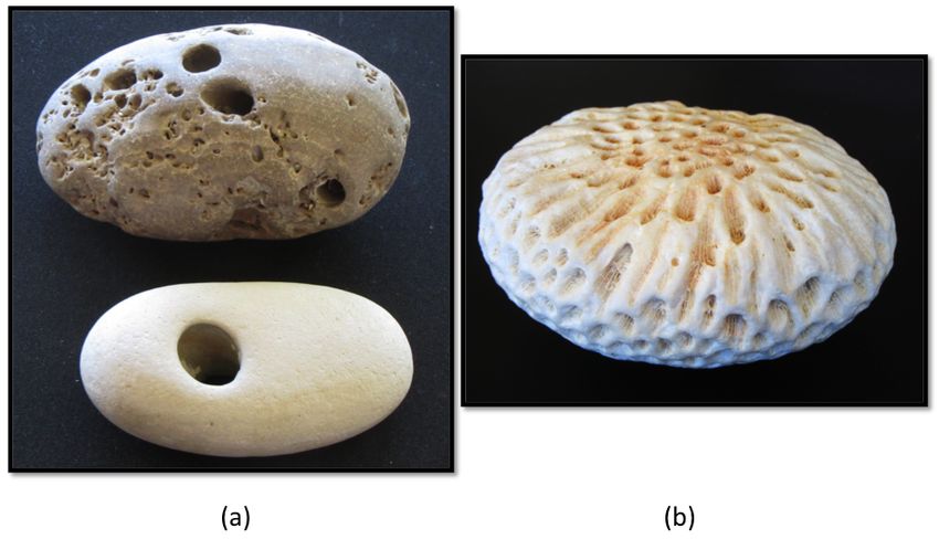
Figure 3: Sketch by Black in 1877 illustrating typical dimensions in the top view (left) and side
view (right) of a hypothetical worn beach stone [8].

beach (left and center) appear to have roughly the same shape independent of size - smaller stones
do not appear to be becoming spherical or cigar-shaped. However, shapes of stones from different
beaches (right) may vary significantly. In fact, the new model presented below predicts exactly this
behavior - that the shapes of stones on the same beach, i.e., subject to the same wave action, tend
to evolve toward the same shape, independent of size; see Example 7.1 below.

    This paper is organized as follows: Section 2 provides an overview of several standard distance-
driven and curvature-driven isotropic models of frictional abrasion of stones, with graphical depic-
tion of numerical solutions of each in the 2-d setting; Section 3 introduces a non-isotropic curvature
and contact-likelihood model of frictional abrasion of beach stones; Section 4 introduces a special
case of this model, with the new geophysical theory and associated equation; Section 5 contains
the definition and essential assumptions concerning the underlying wave process; Section 6 relates
the wave process to the contact-likelihood function; Section 7 analyzes the shape evolution in the
context where both the contact-likelihood function and abrasion are continuous; Section 8 analyzes
the analogous shape evolution in a discrete time and abrasion setting; Section 9 addresses limiting
shapes of abraded stones under the new non-isotropic frictional abrasion model; and Section 10
contains a short conclusion.

2    Classical Isotropic Frictional Abrasion Models
In trying to model the evolving shapes of beach stones, Aristotle conjectured that spherical shapes
dominate (see [15]). In support of his theory, he proposed that the inward rate of abrasion in a
given direction is an increasing function of the distance from the center of mass of the stone to the
tangent plane (the beach) in that direction, the intuition being that the further from the center
of mass a point is, the more likely incremental pieces are to be worn off, since the moment arm is
larger.

                                                  3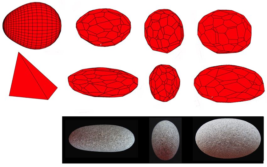
Aristotle’s model may be formalized as follows: (cf. [15, equation (1.1)]; [16, equation (1)]),

                                             ∂h
                                                = −f (h),                                            (1)
                                             ∂t

           where f is an increasing function of the distance h = h(t, u) from the center
            of mass of the stone to the tangent plane in unit direction u at time t.

Figure 4: Numerical simulations* of an egg-shaped and triangular “stone” evolving (a) under
equation (1) with f (h) = h2 , and (b) under (2).

    *NOTE: The curves in Figure 4 and the other figures below were generated in Matlab us-
ing standard semi-implicit curve-shortening techniques (as described in [13]) and random number
(Monte Carlo) generators. These only yield basic approximations of the evolving shapes, not state-
of-the-art renditions. The pseudocode can be found in the Appendix, and the Matlab code for these
numerics may be downloaded at https://hill.math.gatech.edu/DOCUMENTS/stonesCode2.zip.

    Figure 4(a) illustrates numerical solutions of equation (1) in the 2-dimensional setting for tri-
angular and egg-shaped starting shapes for the function f (h) = h2 ; note that in this case shapes
appear to become circular in the limit, which is not the case for some other choices of f , such as
f (h) = h, as will be seen below. Under this model (1), the further from the center of mass, the
faster the stone is eroding. As noted in [15], since the location of the center of gravity is determined
by time-dependent integrals, (1) is a non-local (cf. [25]) partial integro-differential equation.

                                                   4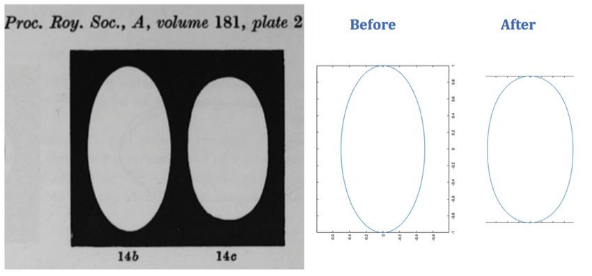
Modern mathematical models for the evolving shapes of stones often assume, as Aristotle did,
that the ablation is normal to the surface of the stone, but unlike Aristotle, they assume that the
rate of ablation is proportional to the curvature at the point of contact. Both Aristotle’s and these
modern models also assume that the stones are undergoing isotropic abrasion, i.e., the stones are
being abraded uniformly from all directions, and each point on the surface of a convex stone is
equally likely to be in contact with the abrasive plane. A typical real-life example of isotropic
frictional abrasion of a stone is the abrasion of a single stone in a standard rock tumbler.
    The assumption that the rate of abrasion at a given point on the surface of the stone is propor-
tional to the curvature at that point is analogous to the assumption that equal volumes (areas) are
ablated in equal time (see Figure 5). This is physically realistic in that sharp points tend to erode
more rapidly than flat regions. Note that under the assumption that the inward rate of abrasion is
proportional to the curvature, the stone in Figure 5 will erode inward at rates less rapidly from A
to C.
    Taking the constant of proportionality to be 1, and using the notation of [20], the basic assump-
tion that the rate of ablation is proportional only to the curvature at the point of contact yields
the classical curvature-driven geometric flow, the local geometric PDE
                                              ∂h0
                                                  = −κ                                              (2)
                                               ∂t

                 where h0 = h0 (t, u) is the distance from a fixed origin to the
                  tangent plane in unit direction u at time t and κ = κ(t, u) is the
                  (Gaussian) curvature of the body in unit direction u at time t.

 The functions h and h0 in (1) and (2) are the support functions of the stone (simple closed curve
or surface) with the origin taken as the center of mass (barycenter) and with the origin fixed,
respectively. As is well-known, the limiting (renormalized) support function h0 under the curve-
shortening flow (2) is constant for essentially all (smooth) convex starting shapes (e.g., [1], [3], and
[20]). Since support functions uniquely determine convex bodies (e.g., [23]), and since spheres are
the only convex bodies with constant support functions (with the origin at the center), this implies
that the shape of a convex stone eroding under (2) becomes spherical in the limit; see Figure 4(b).
(The interested reader is referred to [19] for the evolution of shapes under an even broader class of
curvature-driven geometric flows.)
    Thus the evolution of shapes of stones under frictional abrasion in distance-driven models such
as (1) and curvature-driven models such as (2) are both isotropic, and both are independent of the
shape of the stone away from the point of contact with the beach as well as the underlying wave
dynamics.

3    Non-Isotropic Contact Likelihood
In a physically realistic model of the evolving shape of a stone undergoing frictional abrasion with a
beach, however, both the wave dynamics and the overall shape of the stone play significant roles in
the abrasion process. Intuitively, for instance, if the waves are consistently very small the abrasion
will be minimal and concentrated on the local stable side of the stone, making it flatter. Under
moderate wave action, however, beach stones will become more rounded, as will be seen below.

                                                   5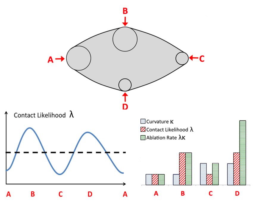
Figure 5: In isotropic curvature-driven frictional abrasion models, ablation is assumed inward
normal to the surface, at a rate proportional to the curvature at the point of contact. Thus if the
curvature κ(A) at the point of contact A is half that at C, κ(C), the rate at which the surface is
being eroded in the normal direction at A is half the rate at C. Note that in Aristotle’s distance-
driven model (1) the relative rates of erosion here are also increasing from A to C, since the distances
from the center of gravity to the point of contact with the abrasive surface are increasing from A
to C.

The basic assumption here is that whenever there is moving contact of the stone with the beach,
friction will occur and the stone will be incrementally abraded at the point of contact.
    As for the shape of the stone playing a role, Rayleigh noted that based on his observations
in nature and in laboratory experiments, “this abrasion cannot be merely a function of the local
curvature” [35, p. 207]. Firey similarly observed that the shape of the stone “surely has a dynamic
effect on the tumbling process and so on the distribution of contact directions at time t” [20, p. 1].
The distance-driven and curvature-driven models (1) and (2) do not provide physically realistic
frameworks for the evolving shapes of stones undergoing frictional abrasion on a flat beach simply
because they are isotropic, that is, they assume that abrasion of the stone is equally likely to occur
in every direction regardless of the shape of the stone and the dynamics of the wave process. Thus,
a more physically realistic model of the evolving shapes of beach stones under frictional abrasion
will necessarily be non-isotropic.
    In particular, in some models like (1) (with f (h) = hα for some α > 1) and (2), a spherical stone
is in stable (attracting) equilibrium, and any shape close to a sphere will become more spherical.
Among real beach stones, however, researchers have reported that “Pebbles never approach the
spherical” [39, p. 211], “one will never find stones in spherical form” [41, p. 1], and “there is little
or no tendency for a pebble of nearly spherical form to get nearer to the sphere” [37, p. 169]. In
fact, Landon reported that “round pebbles become flat” [28, p. 437] and Rayleigh observed “a
tendency to change away from a sphere” [35, p. 114], i.e., that spheres are in unstable (repelling)
equilibrium.
    To see intuitively how a sphere could be in unstable equilibrium under frictional abrasion alone,
consider the thought experiment of the abrasion of a sphere as illustrated in Figure 6. Initially, all
points on the surface of the spherical stone are in equilibrium, and the abrasion is isotropic. But
as soon as a small area has been ablated at a point on the surface, then that flattened direction
is more likely to be in contact with the beach than any other direction, so the abrasion process

                                                   6
now has become non-isotropic. That direction of contact with the beach has now entered stable
equilibrium, as shown at point B in Figure 6. Moreover, since the center of gravity of the ablated
stone has now moved directly away from B, the point A is now also in stable equilibrium, and
the stone is more likely to be ablated at A than at any other point except the B side. Thus, if a
sphere is subject solely to frictional abrasion with a plane (the beach), the abrasion process will
immediately become non-isotropic, and the stone will initially tend to flatten out on two opposite
sides.
Figure 6: In a spherical stone (left) all points on its surface are in unstable equilibrium, with
identical curvatures. As one side is ablated (center) that position now becomes in stable equilibrium,
as does the point A diametrically opposite, and the abrasion process becomes non-isotropic; see
text. Hence the most likely directions for the stone to be ablated next are in directions A and B.
The centers of gravity of the stones from left to right are at c1 , c2 , c3 , respectively.
As mentioned above, in a stone undergoing frictional abrasion on a beach, not only the shape
of the stone, but also the dynamics of the ocean (or lake) waves play a crucial role. If the waves
are consistently very small, the stones will tend to rest in one stable position, and the low energy
of the waves will cause the stones to grind down to a flat face on that side, much like a standard
flat lap polisher is designed to do. The likelihood that other points on the surface of the stone
will come into contact with the abrasive beach plane is very small. At the other extreme, if the
waves are consistently huge, then it is likely that all exposed surface points of the stone will come
into contact with the beach about equally often, i.e., the stone will be undergoing nearly isotropic
abrasion as in a rock tumbler, and will become more spherical.
In the non-isotropic model presented below, an isolated beach stone is eroding as it is being
tossed about by incoming waves (e.g., the beach may be thought of as a plane of sandpaper set
at a slight angle against the incoming waves), and the only process eroding the stone is frictional
abrasion with the beach (e.g., no collisional or precipitation factors as in [9] or [32]). As with the
curvature-driven model (2) above, it is assumed that the rate of ablation per unit time at the point
of contact with the beach is proportional to its curvature at that point – that is, sharp points will
wear faster than flat regions. Unlike a stone eroding in a rock tumbler, the likelihood that abrasive
contact of a stone with a beach occurs in different directions generally depends on both the shape
of the stone and the wave dynamics. That is, in any physically realistic model the ablation process
is not isotropic.
Here it is assumed that the energy required for the frictional abrasion of a beach stone is
7provided solely by the energy of the incoming waves, a time-dependent random process. Thus the
point of contact of the stone with the beach is also a time-varying random variable, and if the
inward ablation of a stone at a given point on its surface is an infinitesimal distance d every time
that point hits the abrasive surface (beach), then in n hits at that point, the resulting inward
abrasion will be nd, the product of the inward rate and the number of times it is abraded at that
point.
Assuming that abrasion is proportional to curvature, this simple product principle implies that
the expected rate of ablation at a point is the product of the curvature there and the average time
that point is in contact with the beach, i.e., the likelihood of contact at that point (for details see
Section 6 below). This suggests the following conceptually natural curvature and contact-likelihood
equation:
∂h
= −λκ (3)
∂t
where h is as in (1), κ is as in (2), and λ = λ(t, u) is the likelihood
of abrasion in unit direction u at time t.
Figure 7 shows a hypothetical convex 2-d stone with the curvatures κ at A and B equal and
exactly half the curvatures at C and D, as depicted by the osculating circles. In isotropic models
of abrasion, where the likelihood function λ is constant (dotted black line), the stone is assumed to
be in contact with the beach with equal frequency (likelihood) at all points on its surface. In the
non-isotropic setting shown (solid blue curve), however, B and D are more often in contact than
A or C. Under the curvature and contact-likelihood model (3), the inward ablation rate at D will
be larger than the rates at A, B, and C.
As will be seen in Section 6 below, λ may be viewed as the local time of the limiting occupation
measure (cf. [22]) of the time-dependent random process that reflects which direction the abrasive
planar beach will be eroding the stone at that time. This crucial contact-likelihood function λ in
(3) may in general be very complicated since it can depend on both the shape of the stone away
from the point of contact, and on the dynamics of the underlying wave process.
4 An Illustrative Model
In cases where the wave process and stone satisfy standard regularity conditions, as will be seen
next, the contact-likelihood function λ may sometimes be approximated by a very simple function
of the distance from the center of mass of the stone. A concrete example of this is λ = h−α for
some α ≥ 1, in which case the basic non-isotropic principle (3) becomes the non-linear partial
integro-differential equation
∂h κ
=− α (4)
∂t h
where h = h(t, u) is as in (1), κ is as in (2), and α ≥ 1.
Thought Experiment for Equation (4).
Consider a single fist-sized non-spherical convex stone (such as one of those in Figures 1 or 2)
8Figure 7: The blue solid curve depicts a typical contact likelihood function for the 2-d “stone”
above under moderate wave action, and the dotted line represents the classical isotropic framework
where all points on the surface of the stone are equally likely to be in contact with the beach. The
graph at right depicts the curvatures, likelihood function values, and the ablation rates predicted
by equation (3) for the points A, B, C, and D. See text.
that is eroding by friction as it is rolled about by waves on a flat sandy beach. Assume that when
a wave comes in, it rolls/lifts the stone to a point of contact with the beach such that the potential
energy of the stone in that position is proportional to the wave crest height - larger waves lift the
center of mass of the stone higher.
Next note that if the expected number of waves needed until the stone comes into contact with
the beach at point B on the surface of the stone is twice the expected number of waves needed until
point A comes into contact, then over time point B will be in contact with the beach half as often
as point A. That is, the likelihood of the stone being in contact with the beach at a given point
on the surface of the stone is proportional to the reciprocal of the expected waiting time to hit that
point.
9Assuming the random wave crest heights follow a Pareto distribution (a standard assumption;
see below), the expected number of waves until a crest of height at least h occurs is proportional to
hα , so the contact-likelihood is proportional to its reciprocal 1/hα . Since the instantaneous rate of
ablation at a point of contact is assumed to be proportional to the curvature κ at that point (again,
sharper points erode faster), taking the constant of proportionality to be 1 gives κ/hα , which yields
the shape evolution equation (4). (More formally, see Section 7 below.)
The novelty of this model (4) is that it considers the product (rather than the sum) of curvature
and distance driven terms and it derives the distance-driven term from the Pareto distribution of
waves.
As suggested in this thought experiment, the new PDE model (4) is only intended to model
the shape evolution of intermediate macroscopic-sized beach stones, not huge boulders or grain-
sized particles. Thus this model is clearly not valid in the limit, where the beach stone eventually
becomes another grain of sand. Also, (4) does not address the changing size of the abrading stone,
which in some river rock models has been shown to decrease exponentially in time (e.g., see [16]
and [33]).
In model (4), the different roles of the three essential rate-of-abrasion factors – curvature at
point of contact, global shape of the stone, and wave dynamics – are readily distinguishable in the
three variables κ, h, and α. The variable κ reflects the curvature at the point of contact, h reflects
the global shape of the stone via its evolving center of mass, and α reflects the intensity of the wave
process (in fact, in the interpretation in Example 7.1 below, α is an explicit decreasing function of
the expected (mean) value of the wave crests). For example, increasing the curvature at the point
of contact affects neither the center of mass nor the wave dynamics, changing the center of mass
affects neither the curvature at the point of contact nor the wave dynamics, and changing the wave
dynamics affects neither the center of mass nor the curvature of the stone.
Figure 8(a) illustrates the same initial 2-d stones shown in Figure 4 evolving under the non-
isotropic curvature and contact-likelihood equation (4) with α = 3; note the similarity of these
oval shapes with the real beach stones in Figures 1 and 2. As will be seen in Section 8 below, this
same prototypical equation model (4) also appears to be robust in both 2-d and 3-d discrete-time
discrete-state “stochastic-slicing” models of the evolution of shapes of beach stones, as illustrated
in Figures 8(b) and 14.
Remark 4.1. Replacing the curvature term κ in equations (2), (3) and (4) by its positive part
κ+ = max{κ, 0} allows those abrasion models to be extended to non-convex initial shapes, and this
is left to the interested reader (see Figure 9).
Remark 4.2. Several other theories have also been proposed to model the evolution of non-
spherical stone shapes. For example, [32] shows the existence of non-spherical limits for a process
that involves a model with a combination of collisional abrasion, frictional abrasion and isotropic
surface growth, and [17] is a PDE model for purely collisional abrasion that also predicts non-
spherical limit shapes. In fact, the evolving shape of the egg-shaped stone in Figure 8(a) is strikingly
similar to Figure 4 in [42], which is based on a model leading to the formation of elliptical stones by
both grinding and rolling abrasion. For an overview of existing models of the geometry of abrasion,
including their history, new extensions, and the mathematical relationship between various models,
the reader is referred to [16].
10Figure 8: Numerical approximations of the shapes of two intermediate-sized 2-d “stones” evolving
(a) under equation (4) with α = 3, and (b) under a discrete chipping analog of (4), as will be
discussed in Section 8. These illustrations depict evolving shapes, not limiting or attracting shapes.
5 Wave Dynamics
The first step in formalizing the fundamental role played by the waves in this non-isotropic curvature
and contact-likelihood frictional abrasion model (3) is to define formally what is meant by a wave
process. Real-life ocean or lake waves are random processes whose components (velocity, direction,
height, temperature, etc.) vary continuously in time. For the purposes of the elementary abrasion
model introduced here, it will be assumed that the critical component of the wave is its energy,
and for simplicity, that this is proportional to its height.
From a realistic standpoint, it is also assumed that wave energies are bounded, i.e., not infinitely
large, and that the wave crests (local maxima) are isolated, that is, no finite time interval contains
an infinite number of crests. These simple notions lead to the following working definition.
Definition 5.1. A wave process W is a bounded, continuous, real-valued stochastic process with
isolated local maxima on an underlying probability space (Ω, F, P ), i.e., W : Ω × R+ → R is such
that:
for each ω ∈ Ω, W (ω, ·) : R+ → R is bounded and
(5)
continuous with isolated local maxima; and
for each t ≥ 0, W (·, t) is a random variable. (6)
11Figure 9: Three isolated beach stones collected by the author illustrate the apparent prevailing
oval shapes of beach stones even when the stone is not homogeneous. The holes in the two stones
in (a) were made by a boring clam triodana crocea in the face of an underwater stationary rock
wall or boulder at Montaña de Oro State Park in California. These oval-shaped “holey” stones
were formed when portions of those rocks with the clam holes broke off and were worn down by
frictional abrasion with the beach. The coral stone in (b) is from a beach cave in Negril, Jamaica.
A standard assumption in oceanography, (e.g., see [12], [30], [34], and [38]), is that the wave
crests have a Pareto distribution. The next example describes a wave process with this property,
and, as seen above, this Pareto distribution plays a key role in the basic heuristics underlying the
physical intuition for equation (4).
Example 5.2. W (t) = Xbtc sin(2πt), where btc = max{n : n ≤ t}, and X1 , X2 , X3 , . . . are i.i.d.
Pareto random variables with c.d.f. P (Xj ≤ x) = 1 − (x0 /x)2 for all x ≥ x0 > 0; see Figure 10. In
contrast to the wave models in [41] and [42], here W is not periodic, as real waves are not, since
the sequence of wave crest heights of W are i.i.d. Pareto random variables.
Note that unlike Brownian motion, which is also a continuous-time continuous-state stochastic
process, a wave process is in general not Markov for the simple reason that the current instantaneous
state of the process alone may not indicate whether the wave is rising or falling.
Another key assumption about the wave process necessary for a physically realistic frictional
abrasion process to follow the curvature and contact-likelihood model (3) is that the long-term
behavior of the wave process is in equilibrium (steady state). To put this in context, recall that for
a continuous function X : R+ → R, the occupation measure (or occupation time of X up to time s)
is the function TX,s = Ts defined by
Z s
Ts (B) = m({0 ≤ t ≤ s : X(t) ∈ B}) = IB (X(t))dt for all Borel B ⊂ R,
0
where m denotes Lebesgue measure on R1 , and IB is the indicator function of B.
12Figure 10: A sample path of a stochastic wave process with Pareto distribution as in Example 5.2.
Note that the process is not periodic, which plays a crucial role in the theory presented here.
Wave Steady-State Assumption
In addition to the wave continuity assumption (5), it is assumed that the wave process {W (ω, t) :
t ≥ 0} has a limiting average occupation measure µW , i.e., there is a Borel probability measure µW
on R satisfying
1
µW (B) = lim m({0 ≤ t ≤ s : W (·, t) ∈ B}) a.s. for all Borel B ⊂ R. (7)
s→∞ s
Note that assumption (7) is essentially a strong law of large numbers, and implies for instance
that W is not going off to infinity, or forever oscillating on average between several different values.
Example 5.3. Suppose W is a wave process with Pareto distribution as in Example 5.2. Then
the maximum heights of the wave intervals {Xj sin(2πt) : t ∈ [j, j + 1); j ≥ 1} are X1 , X2 , . . . ,
respectively, which by assumption are i.i.d. Pareto with P (Xj > x) = (x0 /x)2 for all x ≥ x0 . Thus
by the Glivenko-Cantelli Theorem, the equilibrium limiting distribution of the wave crests of W
has this same Pareto distribution.
6 Contact-Likelihood Function
The next step in relating the underlying wave process W to equation (3) is to describe the relation-
ship of W to the contact-likelihood function λ, which involves the direction of the point of abrasion
on the stone as a function of the underlying time-dependent stochastic wave process W . For ease
of exposition and grapical illustration, in this section “stones” will be depicted in a 2-d setting.
Even for homogeneous and strictly convex stones, the role played by the contact-likelihood
function λ distinguishes the dynamics of the evolution of shape given by the non-isotopic model
(3) from isotropic distance-driven models like (1) and from isotropic curvature-driven models such
as (2), as is illustrated in Figure 7.
A (2-dimensional) stone is a compact convex set K ⊂ R2 with non-empty interior int(K). Let
c = cK ∈ int(K) denote the center of mass (barycenter) of K, and let S 1 denote the unit ball
S 1 = {(x, y) ∈ R2 : x2 + y 2 = 1}.
Definition 6.1. An oriented stone γ is an embedding γ : S 1 → R+ with the origin taken as the
barycenter of the convex hull of the graph of γ. Let S denote the set of all oriented stones.
13The point of abrasion of a stone with the beach as a result of an incoming wave depends not
only on the size and shape of the stone, but also on the wave energy and the orientation of the stone
with the beach when the wave hits. Note that the same wave may act on different orientations of
the same stone to bring it into contact with the beach at different points on its surface.
Definition 6.2. An abrasion direction function D is a continuous function D : S × R → S 1 .
The value D(γ, z) specifies the unit direction of the abrasion plane (the beach) resulting from
a wave with energy z ∈ R acting on the oriented stone γ. In other words, D(γ, z) specifies which
direction of γ will be “down” after γ is hit by a wave with energy z. Figure 11(a) illustrates typical
values of u1 and u2 of the abrasion function D of the oriented stone γ after impact by two waves
with different wave energies z1 and z2 , respectively, resulting in two different points of contact with
the beach, u1 and u2 , at distances h(u1 ) and h(u2 ) from the center of mass.
Figure 11: In (a) an oriented stone γ hit by two different waves with parameters z1 and z2 ,
respectively, results in two different directions of contact with the abrasive plane (beach), u1 =
D(γ, z1 ) and u2 = D(γ, z1 ). Analogously, (b) illustrates the same process in a discrete slicing
framework as will be discussed in Section 8 below.
Recall that m denotes Lebesgue measure.
Proposition 6.3. Given an oriented stone γ, a wave process W , and an abrasion direction function
D, the function Λ = Λ(γ, W, D) : (Ω, F) → [0, 1] given by
1
Λ(B) = lim m({0 ≤ t ≤ s : D(γ, W (·, t)) ∈ B}) for all Borel B ⊂ S 1 (8)
s→∞ s
almost surely defines a Borel probability measure on S 1 .
Proof. Fix a Borel set B in S 1 . Recall by (6) that for all t ≥ 0, W (·, t) is a random variable. By
(5) and Definition 6.2, D(γ, ·) is continuous, and hence Borel measurable, so there exists a Borel
set B̂ in R such that
D(γ, W (·, t)) ∈ B) ⇐⇒ W (·, t) ∈ B̂ for all t ≥ 0. (9)
By the wave steady-state assumption (7), the limit in (8) exists and equals µW (B) a.s., so since
µW is a probability measure, 0 ≤ Λ(B) ≤ 1 a.s. The demonstration that Λ is a.s. a measure is
routine.
14The probability measure Λ in Proposition 6.3 is the occupation measure (cf. [22]) of the steady-
state likelihood (average time) that the oriented stone γ is in contact with the abrasive plane in
various directions, assuming that the rate of abrasion is negligible. For example, if I ∈ S 1 is an
interval of unit directions, then Λ(I) is the probability that the oriented stone γ is in contact with
the beach in direction u for some u ∈ I.
If Λ is absolutely continuous (with respect to Lebesgue measure on S 1 ), then λ, the Radon-
Nikodym derivative of Λ with respect to the uniform distribution on S 1 , is the local time (cf. [7])
of the stochastic process D(γ, W ). That is, λ = dΛ/dm is the density function of the distribution
of the occupation measure. In some instances, as will be seen in the next section, λ may be
approximated by a simple function of γ, in particular, of the support function h of γ.
7 A Model With Continuous Contact-Likelihood and Abrasion
Here, the energy required to produce frictional abrasion of a stone on the beach is assumed to come
only from the waves, which lift and slide the stone against the beach (recall that in this simple
model, collisional abrasion with other stones is assumed negligible). To lift the stone in Figure 12
to abrasion position (c) requires more energy than to lift it to position (b), and (b) requires more
energy than (a). Thus the expected likelihood (or frequency that) the stone is in position (c) is
less than that in (b), and (b) less than (a). This means that for these three points of contact, the
value of the contact-likelihood function λ is decreasing from (a) to (c); the actual numerical values
of λ at these points of course also depend on the external wave process.
Figure 12: The distances h from the center of gravity of the stone in the direction of the normal to
the tangent contact plane are proportional to the potential energies of the stone in that position,
and hence proportional to the wave energy necessary to lift the stone to that position.
Consider a model of the curvature and contact-time ablation equation (3) where the ablation
process is assumed to be continuous in time and space, i.e., a curve-shortening process (cf. [13]).
As before, the incoming wave crest of W lifts the stone to a position determined by the wave
parameters (e.g., kinetic energy of the crest), where its surface is ablated incrementally.
Fix t > 0, and suppose that the oriented stone γ = γ(t) is smooth and strictly convex, i.e., the
non-empty interior of γ is strictly convex with smooth (C ∞ ) boundary. Since the support function
h is continuous, there exist 0 < hmin < hmax < ∞ so that on γ
range(h) = [hmin , hmax ] ⊂ R+ . (10)
15Let Λ denote the occupation measure of the likelihood function of the abrasion direction process
as in Proposition 6.3, and let XΛ denote a random variable with values in the unit sphere and
with distribution Λ, i.e., for all intervals of unit directions I, P (XΛ ∈ I) = Λ(I) represents the
likelihood that γ’s direction of contact with the planar beach at time t is in I. Assuming that
W and D are continuous ((5) and Definition 6.2), it is routine to check that since γ is strictly
convex, the random direction XΛ is absolutely continuous. Thus XΛ has a (Borel) density function
λ : S 1 → R+ satisfying P (XΛ ∈ I) = I λ(u)du for all intervals I ⊂ S 1 .
R
Let YΛ denote the random variable YΛ = mghXΛ , where m is the mass (e.g., volume, or area
in the 2-d setting) of γ and g is the force of gravity. Thus YΛ represents the potential energy of
γ when XΛ is the direction of contact of the stone γ with the abrasive plane, i.e., when XΛ is the
“down” direction at time t. Then (10) implies that
range(YΛ ) = [mghmin , mghmax ] ⊂ R+ . (11)
Assuming that the wave crest energies (relative maxima) are converted into potential energy of
the stone in the corresponding “down” positions (see Figure 12), this implies that the distribution
of YΛ , given that YΛ is in [mghmin , mghmax ], is the same as the distribution of the successive wave
crests of W (see Figure 10) given that they are in [mghmin , mghmax ].
Ignoring secondary effects such as multiple rolls of the stone, this yields an informal physical
explanation for equation (4) with α = 3, as is seen in the next example.
Example 7.1. Suppose that γ is smooth and strictly convex and that W is a wave process as in
Example 5.2, with the {Xj } i.i.d. Pareto random variables satisfying P (Xj > x) = (x0 /x)2 for all
x ≥ x0 for some x0 > 0. Then the sequence X1 , X2 , . . . represents the values of the successive crests
(relative maxima) of W , i.e., Xj = max{W (·, t) : t ∈ [j, j + 1)} (see Figure 10).
This implies that for all x0 < x1 < x2 , the conditional distribution of each Xj given that Xj
has values in [x1 , x2 ] is an absolutely continuous random variable with density proportional to 1/x3
for x ∈ [x1 , x2 ], i.e., there is a c > 0 so that
Z
1
P (Xj ∈ I | Xj ∈ [x1 , x2 ]) = c 3
dx for all I = (a1 , a2 ) ⊂ [x1 , x2 ]. (12)
I x
Letting Yj denote the maximum potential energy of the stone γ during time period [j, j + 1), then
Yj = mgh(Xj ) (see Figure 12). Again assuming that the wave energy at its crests are converted
into potential energy of the stone (see Figure 13), (12) implies that Yj is also absolutely continuous
with density proportional to 1/h3 for h ∈ [hmin , hmax ], so (3) yields (4) with α = 3. Note that
as the stone gets smaller, the factor 1/h3 remains unchanged, but is applied to new values of
hmin and hmax . This suggests that stones of different sizes on the same beach, i.e., subject to the
same (Pareto) wave process, will abrade toward the same (renormalized) shapes; see Figure 2 and
Remark 1.1.
Remark 7.2. Note that the model in (4) is not valid for extremely small values, e.g. when the size
of the beach stone is below the Pareto threshold x0 of the wave. Intuitively, when the beach stone
becomes extremely small, it is comparable to one of the grains of sand that make up the beach,
and is subject to different dynamics such as collisional abrasion and fracturing.
168 A Discrete Contact-likelihood and Abrasion Model
In actual physical frictional abrasion, of course, the evolution of the shape of a stone is not continu-
ous in time, since the ablated portions occur in discrete packets of atoms or molecules. For isotropic
frictional abrasion, this has been studied in [17], [26], and [31], where analysis of the evolution of
the rounding of stones uses Monte Carlo simulation and a “stochastic chipping” process. The goal
of this section is to present an analogous stochastic discrete-time analog of the evolution of a stone’s
shape under the basic isotropic curvature and contact-likelihood equation (4), where again discrete
portions of the stone are removed at discrete steps (see Figure 11(b)), but now where the effects
of both the global shape of the stone (via h) and the wave dynamics (via α) are also taken into
account.
To see how a contact-likelihood function λ may be discrete and explicitly calculated (or approx-
imated), consider the 2-dimensional rectangular “stone” in Figure 13. Without loss of generality,
x1 < x2 and m = 2/g, so the potential energy of the stone in position (a) is x1 and the potential
energy in position (c) is x2 .
Figure 13: A rectangular stone has stable positions of equilibrium shown in (a) and (c); more
energy is required to move the stone from position (a) to (c) than to move it from (c) to (a).
Let W be a Pareto wave process as in Example 5.2; recall Figure 10 for a sample path. Then
the crests (maximum wave heights) of W are the i.i.d. random variables {Xj ; j ∈ N}. Let F̄ denote
the complementary cumulative distribution function of X1 , i.e., F̄ = P (X1 > x) for all x ≥ 0.
Suppose first that the stone is on a longer x2 -side (Figure 13(a)) at time j ∈ N. Then it flips
onto an x1 -side (Figure 13(c)) during the time interval [j, j + 1) if and only if the value of Xj is
greater than the energy required to lift the stone from position (a)√to position (b), i.e., is enough
to increase the potential energy of the stone from x1 to more than x1 2 + x2 2 .
Since the {Xj } are i.i.d., this implies (ignoring multiple flips) that the number of √ waves until
a flip occurs from (a) to (c) is a geometric random variable N1 with parameter F̄ ( x1 2 + x2 2 −
x1 ) := p1 , so the expected value of N1 is E(N1 ) = 1/p1 . Similarly, the expected number of
waves E(N√ 2 ) until a flip occurs from a shorter x1 -side (Figure 13(c)) to an x2 -side is 1/p2 , where
p2 = F̄ ( x1 2 + x2 2 − x2 ) > p1 .
Thus by the strong law of large numbers, the limiting frequency of time that the stone is on
17side x1 is less than the relative frequency of time the stone is on side x2 , since
E(N2 ) 1/p2 p1 p2 E(N1 )
= = < = .
E(N1 ) + E(N2 ) 1/p1 + 1/p2 p1 + p2 p1 + p2 E(N1 ) + E(N2 )
Example 8.1. Suppose the 2-dimensional stone is as in Figure 13 with x1 = 6 and x2 = 8, and
the relative maxima (crests) of the wave process W are as in Example 5.2. Then
c c
p1 = F̄ (4) = 2
> 2 = F̄ (2) = p2 ,
4 2
2
2 /c
so the likelihood that the stone is on a short side (x1 or its opposite side) is 22 /c+4 2 /c = 0.2
and the likelihood the stone is on a long side (x2 or its opposite) is 0.8. This implies that
in terms of the oriented stone as in Figure 13(a), the contact likelihood function λ at time t
satisfies λ(t, (1, 0)) = λ(t, (−1, 0)) = 0.1, λ(t, (0, 1)) = λ(t, (0, −1)) = 0.4, and λ(t, u) = 0 for
u∈/ {(1, 0), (−1, 0), (0, 1), (0, −1)}.
In this setting, as illustrated in Figure 11(b), an oriented stone γ is hit by a wave W resulting in
the unit direction of contact u = D(γ, W ) of γ with the abrasive plane, at which time a small fixed
fraction δ of the volume of the stone is ground off in that direction. (Recall as illustrated in Figure
5 that removing a fixed fraction of the stone in a given direction is analogous to removing a portion
proportional to its curvature there.) The evolving stones in this discrete stochastic framework are
eventually random convex polygons (polyhedra), for which almost every point on the surface has
curvature zero. Thus this assumption that fixed proportions are removed, rather than portions
proportional to curvature, seems physically intuitive.
Figure 8(b) illustrates the results of a Monte Carlo simulation of this stochastic-slicing process
evolving under the discrete-time analog of equation (3) in the special case (4) with α = 3 for the
same two initial 2-d stone shapes as in Figure 4. Here, the direction of ablation is again selected
at random, not uniformly (isotropically), but inversely proportional to the cube of the distance in
that direction from the center of mass to the tangent plane (line). Note the apparent similarity of
the evolving oval shapes in both the continuous and discrete settings, as seen in Figure 8.
An analogous Monte Carlo simulation of this same frictional abrasion process is illustrated in
the 3-d setting in Figure 14 where two initial shapes, a smooth convex egg-shaped body and a non-
regular tetrahedron, are undergoing a discrete-time analog of the same basic non-isotropic curvature
and contact-likelihood model (4) with α = 3. Similar to the analysis in [31] where a discrete-time
stochastic chipping model of the isotropic curvature-driven equation (2) was used to study the rate
at which initial 3-d shapes converge toward spheres, the evolving body here repeatedly has sections
of a fixed proportion δ of the volume removed at each step by a planar cut, in a random direction,
normal to the support function in that direction. In this case, however, in sharp contrast to that
in [31], the abrasion is non-isotropic with the likelihood of abrasion in a given direction inversely
proportional to the cube of the distance from the center of mass of the stone to the supporting
plane in that direction (cf. Example 7.1).
9 Limiting Shapes in a Continuous Abrasion Setting
Recall that, as the numerical approximations in Figure 4(b) illustrated in the 2-d setting, the
limiting shape of stones under curvature-only ablation (2) is spherical, and when normalized, is the
18Figure 14: Monte Carlo simulations, in the 3-d setting, analogous to the 2-d results illustrated in
Figure 8(b), where fixed proportions of the volume are sliced off in random directions, with the
directions chosen inversely proportional to the cube of the distance from the center of mass, i.e.
a discrete analog of (4) with α = 3. For comparison, the corresponding “side”, “end”, and “top”
views of one of the natural beach stones in Figure 2 (right) are shown at bottom.
unit sphere. Similarly, if the contact-likelihood function λ in (3) is constant, then the process is
isotropic and the author conjectures that the limiting shape will also be spherical.
For non-isotropic (non-constant) contact likelihood functions λ, however, the limiting shape
depends on λ, and this shape may sometimes be determined or approximated as follows. First, it
is routine to check that the re-normalized shapes will remain the same if and only if h = h(u, t)
satisfies
∂h
= −ch (13)
∂t
for some c > 0. Equating the term ∂h/∂t in equation (13) with the same term in (3) yields the
shape equation
h
κ=c . (14)
λ
Suppose that the underlying wave crests have a Pareto distribution with α > 1, and that the
ablation process results solely from the conversion of the energy of the wave process W into the
potential energy of the stone, by lifting it to the position where abrasion will occur. Then, as seen
in Example 7.1, λ is proportional to h−α . With (14) this yields the limiting shape equation
κ = chα+1 . (15)
Numerical solutions of (15) for c = 1 and α = 2.5, 3, 4 are shown in Figure 15. Note that flatter
ovals correspond to Pareto waves with smaller means (i.e., with lighter tails), that is, as physical
intuition suggests, more powerful waves produce more spherical limiting shapes.
19Since κ = (h + h00 )−1 , and since h is the distance to the center of mass, note that (15) is a
non-local ordinary differential equation.
Figure 15: Plots of numerical solutions of the limiting shape equation (15) for α = 2.5, 3.0 and 4.0,
respectively.
Note that the oval shapes in Figure 15 appear very similar to the non-elliptical ovals found by
Rayleigh shown in Figure 1 in his empirical data in both natural specimens of beach stones and
in his laboratory experiments. There is also a close resemblance of these same shapes to those in
Fig. 4 of [32], which studies the evolving shapes of carbonate particles that are both growing from
chemical precipitation and eroding from physical abrasion.
The equations for these ovals, the solutions of (15), are not known to the author. Moreover, as
Rayleigh noted, “the principal section of the pebble lies outside the ellipse drawn to the same axes,
and I have not so far found any exception to this rule among artificial pebbles shaped by mutual
attrition, or among natural pebbles” [36].
Figure 16: Actual before and after shapes (left) of a stone worn by frictional abrasion in a laboratory,
as recorded by Lord Rayleigh in 1942. Rayleigh specifically noted that the limiting shapes are not
ellipses, and demonstrated this experimentally by starting with a stone with an elliptical shape
(14b), which after ablation assumed the non-elliptical shape shown in (14c) [35]. The graphics on
the right illustrate how closely a numerical solution to equation (4) with α = 2.2 approximates his
findings in a 2-d setting.
20More concretely, Figure 16 illustrates the limiting shapes predicted by the prototypical model
in equation (4) with the empirical laboratory data reported by Rayleigh [35]. The stone (14b) in
Figure 16 is the near-elliptical actual stone he subjected to frictional abrasion, and to its right (14c)
is the same stone after ablation. In the two curves on the right in Figure 16, the one on the left
is an exact ellipse with minor axis 0.5 and major axis 1.0 centered at the origin, and to its right
is the evolved shape after curve shortening via the curvature and contact-likelihood equation (4)
with α = 2.2. Note the striking resemblance of the experimental results with the model presented
in the simple equation (3) with λ = h−α .
Also note that the chipping process depicted in Figure 14, even when renormalized at each step,
does not have a limiting shape since at each successive iteration a fixed proportion of the volume is
chipped off. In this scenario the author conjectures that there is a limiting distribution of (convex
polyhedral) shapes, and those illustrated in Figure 14 are representative cases.
10 Conclusions
The non-isotropic model of the evolution of the shapes of beach stones introduced here is meant
as a starting point to include the effects of both the global (non-local) shape of the stone and the
wave dynamics into the process. The main equations are simple to state, but as non-local partial
integro-differential equations, they are difficult to solve exactly, and no solutions are known to the
author. Numerical approximations in the continuous-time continuous-state framework using stan-
dard curve-shortening algorithms, and in the discrete-time discrete-state framework using Monte
Carlo simulation, both indicate remarkably good agreement with the shapes of both natural and
artificial stones undergoing frictional abrasion on a flat plane.
Acknowledgements
The author is grateful to Professors Pieter Allaart, Arno Berger, Gábor Domokos, Lester Dubins,
Ron Fox, Ryan Hynd, Kent Morrison, and Sergei Tabachnikov for many helpful comments, to
Professor Donald Priour for access to his 3-d “stochastic-chipping” code, to an anonymous referee
for many corrections and helpful suggestions, and especially to John Zhang for his excellent work on
the Monte Carlo simulations and curve-shortening numerics presented here, and for many helpful
ideas, suggestions, and questions.
References
[1] Andrews, B. Evolving convex curves. Calc. Var. Partial Differential Equations 7, 4 (1998),
315–371.
[2] Andrews, B. Gauss curvature flow: the fate of the rolling stones. Invent. Math. 138, 1
(1999), 151–161.
[3] Andrews, B. Classification of limiting shapes for isotropic curve flows. J. Amer. Math. Soc.
16, 2 (2002), 443–459.
[4] Andrews, B., McCoy, J., and Zheng, Y. Contracting convex hypersurfaces by curvature.
Calc. Var. Partial Differential Equations 47, 3–4 (2013), 611–665.
21[5] Aristotle. Mechanica. In The Oxford translation of the complete works of Aristotle, W. D.
Ross, Ed., vol. 6. Clarendon Press, Oxford, 1913.
[6] Ashcroft, W. Beach pebbles explained. Nature 346, 6281 (1990), 227–227.
[7] Björk, T. The pedestrian’s guide to local time, 2015.
[8] Black, W. T. On rolled pebbles from the beach at Dunbar. Transactions of the Edinburgh
Geological Society 3, 1 (1877), 122–123.
[9] Bloore, F. J. The shape of pebbles. Journal of the International Association for Mathemat-
ical Geology 9, 2 (1977), 113–122.
[10] Bluck, B. J. Sedimentation of beach gravels: Examples from South Wales. J. Sediment.
Res. 37, 1 (1967), 128–156.
[11] Carr, A. P. Size grading along a pebble beach: Chesil Beach, England. J. Sediment. Res.
39, 1 (1969), 297–311.
[12] Chen, B.-y., Zhang, K.-y., Wang, L.-p., Jiang, S., and Liu, G.-l. Generalized Extreme
Value-Pareto Distribution Function and Its Applications in Ocean Engineering. China Ocean
Eng. 33, 2 (2019), 127–136.
[13] Deckelnick, K., and Dziuk, G. On the approximation of the curve shortening flow. In
Calculus of Variations, Applications and Computations, C. Bandle, M. Chipot, J. S. J. Paulin,
J. Bemelmans, and I. Shafrir, Eds. Longman Scientific & Technical, Essex, U.K., 1994, pp. 100–
108. Pont-à-Mousson.
[14] Dobkins, Jr., J. E., and Folk, R. L. Shape development on Tahiti-Nui. J. Sediment. Res.
40, 4 (1970), 1167–1203.
[15] Domokos, G., and Gibbons, G. W. The evolution of pebble size and shape in space and
time. Proc. Math. Phys. Eng. Sci. 468, 2146 (2012), 3059–3079.
[16] Domokos, G., and Gibbons, G. W. The Geometry of Abrasion. In New Trends in Intuitive
Geometry, G. Ambrus, I. Bárány, K. J. Böröczky, G. F. Tóth, and J. Pach, Eds., vol. 27 of
Bolyai Society Mathematical Studies. János Bolyai Mathematical Society and Springer-Verlag
GmbH, Budapest, 2018, pp. 125–153.
[17] Domokos, G., Sipos, A. Á., and Várkonyi, P. L. Countinuous and discrete models for
abrasion processes. Periodica Polytechnica Architecture 40, 1 (2009), 3–8.
[18] Durian, D. J., Bideaud, H., Duringer, P., Schröder, A., Thalmann, F., and Mar-
ques, C. M. What is in a pebble shape? Phys. Rev. Lett. 97 (Jul 2006), 028001.
[19] Fehér, E., Domokos, G., and Krasukopf, B. Computing critical point evolution under
planar curvature flows, 2020.
[20] Firey, W. J. Shapes of worn stones. Mathematika 21, 41 (1974), 1–11.
[21] Gage, M. E. Curve shortening makes convex curves circular. Invent. Math. 76, 2 (1984),
357–364.
22[22] Geman, D., and Horowitz, J. Occupation densities. Ann. Probab. 8, 1 (1980), 1–67.
[23] Ghosh, P. K., and Kumar, K. V. Support function representation of convex bodies, its
application in geometric computing, and some related representations. Comput. Vis. Image
Underst. 72, 3 (1998), 379–403.
[24] Hamilton, R. S. Worn stones with flat sides. Discourses Math. Appl. 3 (1994), 69–78.
[25] Kavallaris, N. I., and Suzuki, T. Non-Local Partial Differential Equations for Engineering
and Biology. Springer International Publishing, Cham, Switzerland, 2018.
[26] Krapivsky, P. L., and Redner, S. Smoothing a rock by chipping. Phys. Rev. E 75 (Mar
2007), 031119.
[27] Krynine, P. D. On the antiquity of “sedimentation” and hydrology (with Some Moral
Conclusions). Geol Soc Am Bull. 71, 11 (1960), 1721–1726.
[28] Landon, R. E. An analysis of beach pebble abrasion and transportation. J. Geol. 38, 5
(1930), 437–446.
[29] Lorang, M. S., and Komar, P. D. Pebble shape. Nature 347, 6292 (1990), 433–434.
[30] Mackay, E. B. L., Challenor, P. G., and Bahaj, A. S. A comparison of estimators for
the generalised Pareto distribution. Ocean Eng. 38 (2011), 1338–1346.
[31] Priour, Jr., D. J. Time scales for rounding of rocks through stochastic chipping, 2020.
[32] Sipos, A. A., Domokos, G., and Jerolmack, D. J. Shape evolution of ooids: a geometric
model. Sci. Rep. 8, 1 (2018), 1758.
[33] Sipos, A. A., Domokos, G., and Török, J. Particle size dynamics in abrading pebble
populations. Earth Surf. Dynam. 9, 2 (2021), 235–251.
[34] Stansell, P. Distributions of extreme wave, crest and trough heights measured in the North
Sea. Ocean Eng. 32, 8 (2005), 1015–1036.
[35] Strutt (Lord Rayleigh), R. J. The ultimate shape of pebbles, natural and artificial. Proc.
Math. Phys. Eng. Sci. 181, 985 (1942), 107–118.
[36] Strutt (Lord Rayleigh), R. J. Pebbles, natural and artificial, their shape under various
conditions of abrasion. Proc. Math. Phys. Eng. Sci. 182, 991 (1944), 321–335.
[37] Strutt (Lord Rayleigh), R. J. Pebbles of regular shape and their production in experi-
ment. Nature 154, 3901 (August 1944), 169–171.
[38] Teixeira, R., Nogal, M., and O’Connor, A. On the suitability of the generalized Pareto
to model extreme waves. Journal of Hydraulic Research 56, 6 (2018), 755–770.
[39] Wald, Q. R. The form of pebbles. Nature 345 (1990), 211.
[40] Williams, A. T., and Caldwell, N. E. Particle size and shape in pebble-beach sedimen-
tation. Mar. Geol. 82, 3 (1988), 199–215.
23You can also read