Forcing mechanisms of the migrating quarterdiurnal tide - ANGEO
←
→
Page content transcription
If your browser does not render page correctly, please read the page content below
Ann. Geophys., 38, 527–544, 2020
https://doi.org/10.5194/angeo-38-527-2020
© Author(s) 2020. This work is distributed under
the Creative Commons Attribution 4.0 License.

Forcing mechanisms of the migrating quarterdiurnal tide
Christoph Geißler, Christoph Jacobi, and Friederike Lilienthal
Institute for Meteorology, Universität Leipzig, Stephanstr. 3, 04103 Leipzig, Germany

Correspondence: Christoph Geißler (christoph.geissler@uni-leipzig.de)

Received: 8 October 2019 – Discussion started: 28 October 2019
Revised: 18 March 2020 – Accepted: 21 March 2020 – Published: 20 April 2020

Abstract. We used a nonlinear mechanistic global circu-          et al., 1987) and reach a maximum in the MLT region before
lation model to analyze the migrating quarterdiurnal tide        they dissipate. Tides with larger periods like diurnal tides
(QDT) in the middle atmosphere with focus on its possi-          (DTs), semidiurnal tides (SDTs) and terdiurnal tides (TDTs)
ble forcing mechanisms: the absorption of solar radiation        usually have larger amplitudes than short-period tides like the
by ozone and water vapor, nonlinear tidal interactions, and      quarterdiurnal tide (QDT). This is why the QDT has attracted
gravity wave–tide interactions. We show a climatology of         less attention in the past than the relatively well understood
the QDT amplitudes, and we examine the contribution of           DTs, SDTs and TDTs.
the different forcing mechanisms to the QDT amplitude. To           There are few observational and model studies available
this end, we first extracted the QDT from the model ten-         on the QDT; however, the QDT has been observed from
dency terms and then removed the respective QDT contri-          satellites. Therefore, Azeem et al. (2016) analyzed tem-
bution from the different tendency terms. We find that the       perature data from the near-infrared spectrometer (NIRS)
solar forcing mechanism is the most important one for the        onboard the International Space Station (ISS) and from
QDT; however, the nonlinear and gravity wave forcing mech-       the Sounding of the Atmosphere using Broadband Emis-
anisms also play a role in autumn and winter, particularly at    sion Radiometry (SABER) instrument onboard the Ther-
lower and middle latitudes in the mesosphere and lower ther-     mosphere Ionosphere Mesosphere Energetics Dynamics
mosphere. Furthermore, destructive interference between the      (TIMED) satellite. They obtained an amplitude of the QDT
individual forcing mechanisms is observed. Therefore, tidal      that grew from ∼ 5 K near an altitude of 100 km to ∼ 30 K
amplitudes become even larger in simulations with the non-       near an altitude of 130 km. Liu et al. (2015) also used mea-
linear or gravity wave forcing mechanisms removed.               surements from SABER/TIMED temperature data to analyze
                                                                 the QDT in the MLT as well as its global structure and sea-
                                                                 sonal variability. They compared their results with different
                                                                 Hough modes. In their study, they noticed that between an al-
1   Introduction                                                 titude of 70 and 90 km at the Equator and at low latitudes, the
                                                                 (4,6) Hough mode dominated; above 90 km, more than one
The dynamics of the upper mesosphere and lower thermo-           Hough mode is visible, but the (4,6) mode remains predomi-
sphere (MLT) are strongly influenced by atmospheric waves,       nant. The SABER/TIMED data also show a meridional struc-
especially solar tides (Forbes, 1982a, b; Forbes et al., 1994;   ture with three amplitude maxima between 4◦ S and 4◦ N:
Manson et al., 1989; Hagan et al., 1995; Jacobi et al., 1999;    two of these maxima are centered at 3◦ and one is centered
Pancheva et al., 2002; Yiğit and Medvedev, 2015). Tides are     above the Equator. This structure is also seen in the analy-
global-scale oscillations with periods of a solar day (24 h)     ses by Azeem et al. (2016) with two additional maxima at
and its harmonics (12, 8 and 6 h), which mainly result from      about 6◦ in both hemispheres. Jacobi et al. (2019) analyzed
the absorption of solar radiation by water vapor in the tropo-   QDT signatures in lower ionospheric sporadic E occurrence
sphere and ozone in the stratosphere (Chapman and S., 1970;      rates. They mainly found maxima during early and late win-
Andrews et al., 1987; Xu et al., 2012). Because of the de-       ter at middle latitudes, which coincided with modeled verti-
crease in density and conservation of energy, the tidal ampli-   cal shear QDT maxima of the zonal wind.
tudes increase with height (Chapman and S., 1970; Andrews

Published by Copernicus Publications on behalf of the European Geosciences Union.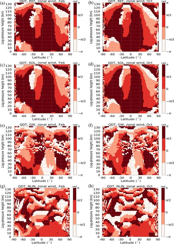
528                                             C. Geißler et al.: Forcing mechanisms of the migrating quarterdiurnal tide

   The QDT has also been observed in radar wind mea-              these forcing mechanisms and their relative contribution to
surements in the MLT region (e.g., Sivjee and Walterscheid,       the QDT tidal amplitudes. The paper is structured as fol-
1994; Smith et al., 2004; Jacobi et al., 2017b; Guharay et al.,   lows: the model and experiments are described in Sect. 2; the
2018). Guharay et al. (2018) analyzed the variability of the      QDT model climatology is presented, and the results of the
QDT in the MLT over Brazilian low-latitude stations and           runs with different forcing mechanisms excluded are shown
found QDT wind amplitudes that reach 2 ms−1 with a max-           in Sect. 3; and finally, the results are discussed and summa-
imum during late summer and fall. Jacobi et al. (2017b)           rized in Sect. 4.
analyzed MLT (80–100 km) radar data from Collm (51◦ N,
13◦ E) and Obninsk (55◦ N, 37◦ E). They found maximum
amplitudes in winter with a long-term mean monthly mean           2   Description of the model and the experiments
zonal amplitude of 7 ms−1 . Bispectrum analysis of the Collm
data showed that nonlinear interaction is a possible forcing      The Middle and Upper Atmosphere Model (MUAM;
mechanism, especially in winter and in the upper height gates     Pogoreltsev, 2007; Pogoreltsev et al., 2007) is used to in-
accessible to the radar (Jacobi et al., 2018). MLT radar ob-      vestigate the forcing mechanisms of migrating QDTs with
servations were also performed at Esrange (68◦ N, 21◦ E)          wave number 4. MUAM is a 3-D, primitive equation, mech-
by Smith et al. (2004). They observed maximum monthly             anistic global circulation model based on the earlier Cologne
mean amplitudes during winter that can exceed 5 ms−1 . They       Model of the Middle Atmosphere–Leipzig Institute for Mete-
also presented simulations of the QDT using a mechanistic         orology (COMMA-LIM), described by Jakobs et al. (1986),
model, which supported the results from the radar at Esrange      Fröhlich et al. (2003b) and Jacobi et al. (2006). Recent ver-
and Collm, showing similar timing and magnitude of the sea-       sions of the MUAM model are described by Lilienthal et al.
sonal peak amplitude. Furthermore, Smith et al. (2004) ana-       (2017), Lilienthal et al. (2018), Lilienthal and Jacobi (2019),
lyzed the forcing mechanisms of the QDT and showed that           Jacobi et al. (2019) and Samtleben et al. (2019). The model
the solar forcing mechanism is the most important. Never-         reaches from the surface at 1000 hPa to a log-pressure height
theless, there is also a possible influence from a nonlinear      of 160 km, with a constant scale height of H = 7 km and a
interaction between different tides that may cause an addi-       vertical resolution of 2.842 km. In the lowermost 30 km, i.e.,
tional QDT to the solar-forced QDT. The theory of nonlinear       in the lowest 10 model levels, the zonal mean temperatures
interactions between tides was described by Teitelbaum and        are nudged to monthly mean zonal mean ERA-Interim re-
Vial (1991). Accordingly, a pure nonlinear QDT wave (pe-          analysis temperatures (ERA-Interim, 2018; Dee et al., 2011).
riod of 6 h) is generated when a nonlinear interaction occurs     The wave propagation remains unaffected by nudging, as this
between two SDTs (periods of 12 h) or between a TDT and           only alters the zonal mean. Above 30 km, the background
a DT (periods of 8 and 24 h). Similarly, it holds for the wave    winds can develop freely in the model and are only affected
number k, that a k = 4 wave can be formed by a nonlinear in-      by the zonal mean temperature nudging below. In contrast
teraction between two existing waves with k = 2 or between        to other model experiments (e.g., Pogoreltsev et al., 2007;
waves with k = 1 and k = 3. Another possible source of tides      Pogoreltsev, 2007; Lilienthal et al., 2017; Samtleben et al.,
is the interaction between gravity waves and tides. For ex-       2019), we do not include planetary wave forcing at the lower
ample, Miyahara and Forbes (1991) demonstrated such a             boundary to avoid undesired wave coupling with tides. In our
mechanism for the TDT, although without consideration of          experiments, we perform ensemble runs with 11 members
the QDT. Simulations of gravity wave–tide interactions were       using ERA-Interim data from 2000 to 2010 in order to de-
performed by Ribstein and Achatz (2016), but they did not         scribe interannual variability.
analyze higher harmonics than the SDT. Liu et al. (2006)             The solar heating through absorption, including water va-
showed nonlinear interactions between atmospheric tides at        por, carbon dioxide, ozone, oxygen and nitrogen, in the mid-
midlatitude radar measurements, as well as an interaction be-     dle atmosphere is parameterized following Strobel (1978).
tween tides and gravity waves from a bicoherence spectrum         We do not intend to perform an ozone- and CO2 -dependent
analysis. This was mainly found for the upper height gates        trend analysis, so we leave both constant in all simula-
considered.                                                       tions. Ozone is implemented as a monthly mean zonal
   To summarize, there is some indication that the QDT is a       mean field for the year 2005 up to an altitude of 50 km
regular phenomenon especially visible in the MLT, but the         taken from MERRA-2 (Modern-Era Retrospective Analy-
database is sparse and there is no final and quantitative in-     sis for Research and Applications, version 2) reanalysis data
formation about the role of its different forcing mechanisms.     (MERRA-2, 2019; Gelaro et al., 2017) for each of the en-
Therefore, in this paper, we analyze the migrating QDT in         semble members. Above 50 km, the ozone mixing ratio is
the middle atmosphere with the help of a mechanistic global       assumed to decrease exponentially. In the ensemble runs, the
circulation model, and we focus on possible forcing mech-         CO2 mixing ratio is chosen according to the Mauna Loa Ob-
anisms, i.e., the absorption of solar radiation by ozone and      servatory data for 2005 as a global constant up to 80 km and
water vapor, nonlinear tidal interaction, and gravity wave–       an exponential decrease above this level (e.g., 380 ppm for
tide interaction. This is carried out by separately analyzing     February 2005; NOAA ESRL Global Monitoring Division,

Ann. Geophys., 38, 527–544, 2020                                                          www.ann-geophys.net/38/527/2020/
C. Geißler et al.: Forcing mechanisms of the migrating quarterdiurnal tide 529
2018; Thoning et al., 1989). Extreme ultraviolet (EUV) and Solar tides, including the QDT, may be generated by three
chemical heating (Riese et al., 1994) are included (Fröhlich different mechanisms, namely solar heating, nonlinear tide–
et al., 2003a). tide interactions, and gravity wave–tide interactions. More
The diurnal cycle of solar radiation absorption leads details on these forcing mechanisms and how they are rep-
to self-consistent forcing of tidal harmonics such as DT, resented in the MUAM model are described by Lilienthal
SDT, TDT and QDT. The model is unable to produce non- et al. (2018). Here, we essentially follow their approach by
migrating tides, because it contains no 3-D fields of ozone removing different forcing mechanisms. To this end, we used
and water vapor – it only contains zonal means. In contrast a Fourier transform and removed the wave number 4 (which
to the version by Ermakova et al. (2017) and Jacobi et al. is equivalent to the migrating QDT, as there are no non-zonal
(2017a), latent heat release is not included here. We used a structures except for the migrating tides in our MUAM ver-
horizontal resolution of 2.5◦ × 5.625◦ for the model, which sion) amplitude from the respective forcing term during each
differs from the version of, e.g., Lilienthal et al. (2017) and time step and at each model grid point. To remove the solar
Lilienthal et al. (2018), in order to be able to better resolve forcing mechanism, the wave number 4 heating was removed
the meridional structure of the QDT. In an earlier model ver- from the radiation parameterization scheme. To remove the
sion with a 5◦ meridional resolution, essentially only one nonlinear tide–tide interactions, we separated the nonlinear
maximum was seen in the QDT amplitudes per hemisphere terms, which are essentially the advection terms in the mo-
(Jacobi et al., 2019), whereas satellite observations (Azeem mentum equation and the temperature equation, as was done
et al., 2016; Liu et al., 2015) show a more detailed merid- in Lilienthal et al. (2018). We then removed the wave num-
ional structure. Furthermore, from the linear theory, includ- ber 4 in these terms. As these advection terms are responsi-
ing the QDT meridional structure representation by Hough ble for wave–wave interactions, this strategy effectively re-
modes, another result was expected, as shown by Azeem moves the QDT forcing through nonlinear interaction. To re-
et al. (2016). move gravity wave–tide interactions, the total acceleration
The gravity wave routine, which is used in this model and heating through gravity wave oscillations of wave num-
version, is an updated linear Lindzen-type parameterization ber 4 are removed. Table 1 shows an overview of our simu-
(Lindzen, 1981; Jakobs et al., 1986), as described by Fröhlich lations in which different forcing mechanisms are eliminated
et al. (2003b) and Jacobi et al. (2006). This parameterization separately: (i) SOL, which had no gravity wave–tide interac-
is based on waves initialized at an altitude of 10 km that are tions and no nonlinear interactions; (ii) NLIN, which had no
traveling in eight directions with a phase speed between 5 solar forcing mechanism and no gravity wave–tide interac-
and 30 ms−1 . These waves do not effectively propagate be- tions; and (iii) GW, which had no solar forcing and no non-
yond the lowermost thermosphere; therefore, the Lindzen- linear interactions. Effectively, these experiments represent
type routine is coupled through the eddy diffusion coeffi- model runs with only solar (SOL), nonlinear (NLIN) and
cient with a modified nonlinear parameterization, follow- gravity wave (GW) forcing of the QDT. Furthermore, two
ing Yiğit et al. (2008, 2009), which is initiated with gravity experiments were performed where only one process was re-
waves of higher horizontal phase speeds. The individually moved, namely (iv) NO_NLIN with removed nonlinear inter-
excited gravity waves are clearly separated by their differ- actions, and (v) NO_GW without gravity wave–tide interac-
ent phase velocities. The distribution of tendency terms from tion. In addition, a reference (REF) run was performed with
both gravity wave routines can be summed up to the total ac- all forcing mechanisms enabled.
celeration of the mean flow through gravity waves. More in-
formation about the gravity wave parameterization included
in MUAM is given in Lilienthal et al. (2017) and Lilienthal 3 Results
et al. (2018).
The model uses a time step of 120 s and starts with a spin- 3.1 Reference simulation and QDT climatology
up time of 120 model days. In that time, the heating rates are
zonally averaged, which means there are no tides. After that, In the reference run (REF), all forcing mechanisms (direct
a further 90 model days are simulated with zonally variable solar, gravity wave–tide interactions and nonlinear interac-
heating rates so that tidal forcing is introduced. The decli- tions) are included. Results from this experiment will be de-
nation in this model version is fixed to the 15th day of the scribed here in comparison with results from the literature.
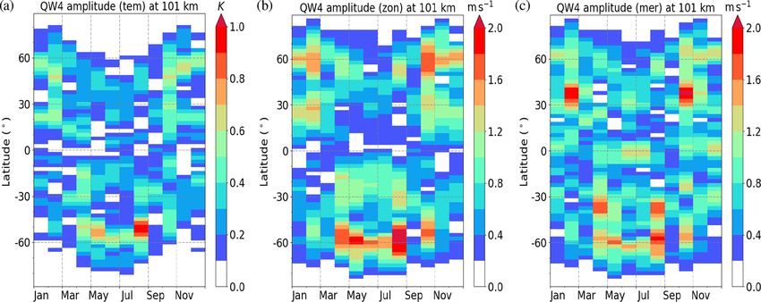
respective month. The following results are analyzed from For an overview of the seasonal cycle of the QDT, Fig. 1
the last 30 model days. In this time period, the tidal am- shows the QDT temperature and wind amplitudes at a height
plitudes remain almost constant and show only small day- of about 101 km. In the Northern Hemisphere, amplitudes in-
to-day variations. Lower atmospheric mean temperatures are crease in autumn and winter in the latitude ranges from 20 to
nudged during the entire model run. However, as only zonal 40◦ N and from 50 to 70◦ N, respectively. Maximum wind
means are modified, tidal forcing and propagation remains amplitudes in the Northern Hemisphere are seen in February
possible. and October; for the meridional wind, the largest amplitudes
are found in the 20–40◦ N range, whereas the largest zonal
www.ann-geophys.net/38/527/2020/ Ann. Geophys., 38, 527–544, 2020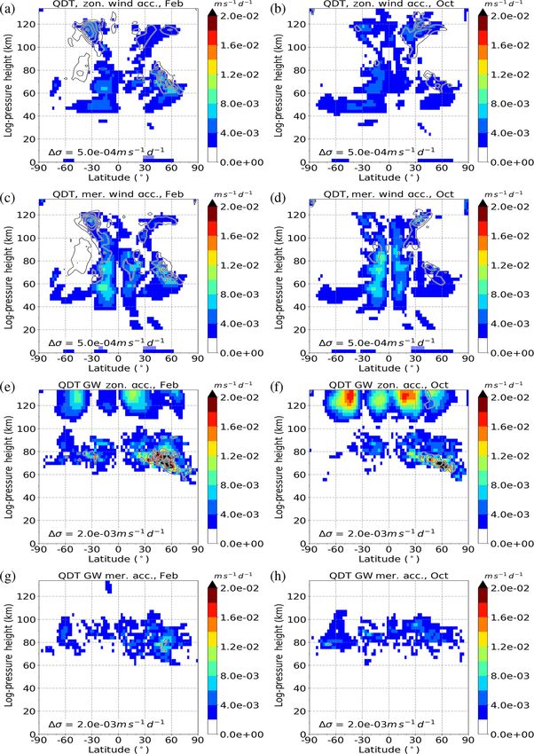
530 C. Geißler et al.: Forcing mechanisms of the migrating quarterdiurnal tide
Table 1. Overview on the different model experiments.
Simulation Description Solar Nonlinear Gravity wave
forcing forcing forcing
SOL Removed nonlinear and gravity wave forcing On Off Off
NLIN Removed solar and gravity wave forcing Off On Off
GW Removed solar and nonlinear forcing Off Off On
NO_NLIN Removed nonlinear forcing On Off On
NO_GW Removed gravity wave forcing On On Off
REF Reference with all forcings On On On
wind and temperature QDT amplitudes during these months plitudes with altitude is correctly reproduced by the MUAM
are seen at 50–70◦ N. In the Southern Hemisphere maximum model. However, the maxima of the DT and SDT amplitudes
amplitudes also appear during autumn and winter (April to in MUAM are sometimes more than 50 % lower than those
October) between 20–40 and 50–70◦ S. The higher latitude of the GSWM at low- and midlatitudes. Furthermore, com-
maximum is more strongly expressed than in the Northern parison with radar measurements (e.g., Manson et al., 1989;
Hemisphere. Pokhotelov et al., 2018) shows that the amplitudes of the DT
Liu et al. (2015) showed a climatology of QDT tempera- and SDT are underestimated in MUAM.
ture amplitudes from SABER/TIMED satellite data between Meteor radar measurements of zonal wind QDT ampli-
50◦ N and 50◦ S over 10 years. The amplitudes presented by tudes at 50◦ N by Jacobi et al. (2017b, 2018) show max-
Liu et al. (2015) show maxima near 30◦ N and 30◦ S and ima in January and February as well as in April and May,
above the Equator. Their QDT temperature amplitudes reach which is analogous to the MUAM simulations. The maxima
values from 0.5 to 1.0 K between 70 and 90 km, and the am- in autumn, seen in Fig. 1b, are also supported by their mea-
plitudes reach up to 4 K on an annual and long-term aver- surements. Moreover, the temporal and spatial distribution of
age at higher altitudes. Thus, the amplitudes observed by Liu zonal wind amplitudes by Smith et al. (2004) show good sim-
et al. (2015) are larger than those in the MUAM simulation. ilarity in with the MUAM simulations, as is also the case for
The maxima in February, April, May and August at 40◦ N the meridional wind amplitudes in our study (Fig. 1c).
from MUAM simulations in Fig. 1a agree with the satellite Ensemble simulations, which contain the solar, nonlinear
measurements analyzed by Liu et al. (2015). Our simulated and gravity wave forcing mechanisms for all wave numbers,
maximum in October, in comparison, does not appear in the are useful as a reference for all experiments because they rep-
SABER/TIMED data. Moreover, the extrema at about 10◦ N resent a QDT that can be compared with observations. The
in June, September and October, as reported by Liu et al. results in the following are given as means of the 11 ensem-
(2015), do not match with the MUAM results, because the ble members. As the largest amplitudes are found in Febru-
amplitudes in the model are much smaller than the ampli- ary and October in the Northern Hemisphere (see Fig. 1),
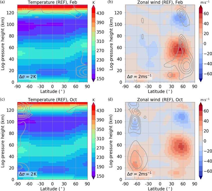
tudes observed by satellites. we selected these months for further analysis. In Fig. 2, the
Model simulations of the QDT temperature amplitudes at background climatology for the MUAM zonal mean circula-
an altitude of 100 km by Smith et al. (2004) show a similar tion is shown for February (Fig. 2a, b) and October (Fig. 2c,
seasonal and latitudinal amplitude maximum distribution as d), for the temperature (Fig. 2a, c) and zonal wind (Fig. 2b,
seen in the MUAM results. Again, however, the amplitudes d) parameters. The data are the model results for the years
in the model simulations from Smith et al. (2004) are larger 2000–2010 (shown using color coding), i.e., with the respec-
than in the MUAM results. Amplitudes in the MUAM simu- tive ERA-Interim reanalysis zonal mean temperatures used
lations tend to underestimate other results by a factor of about for nudging, and are presented with the corresponding stan-
2 or 3. One reason for this is that water vapor in MUAM is dard deviations (shown using contour lines).
implemented as zonal mean and not as a 3-D field, and latent The model zonal wind climatology agrees reasonably well
heat is also not included as a QDT source in the model. In with earlier empirical climatologies such as COSPAR Inter-
addition, the amplitudes of other tides (DT, SDT and TDT) national Reference Atmosphere (CIRA-86; Fleming et al.,
are also too small compared with observations (Lilienthal 1990) or the radar-based Global Empirical Wind Model
et al., 2018); thus, nonlinear interaction processes are possi- (GEWM; Portnyagin et al., 2004; Jacobi et al., 2009) and the
bly underestimated. Figure S5 in the Supplement shows the satellite-based URAS Reference Atmosphere Project (URAP
DT and SDT zonal wind amplitudes for February and Octo- Swinbank and Ortland, 2003). In February, the easterly jet
ber from the MUAM REF simulation as well as the clima- of the summer hemisphere is weaker than the abovemen-
tology from the Global Scale Wave Model (GSWM, 2020). tioned climatologies. The same is true for the equatorial east-
The latitude-dependent structure and the increase of the am- erly winds in October. The model temperature shows gen-
Ann. Geophys., 38, 527–544, 2020 www.ann-geophys.net/38/527/2020/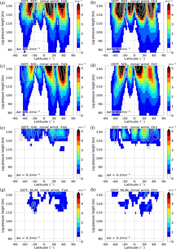
C. Geißler et al.: Forcing mechanisms of the migrating quarterdiurnal tide                                                           531

Figure 1. REF monthly mean QDT amplitudes at an altitude of 101 km. From left to right: (a) temperature, (b) zonal wind and (c) meridional
wind.

Figure 2. Panels (a) and (c) show the REF zonal mean temperature, and panels (b) and (d) show zonal wind for (a, b) February and (c, d)
October conditions. Results are an average of 11 ensemble members (shaded color). Standard deviations σ are 2 K for temperature and
2 ms−1 for zonal wind.

eral agreement with the empirical CIRA-86 climatology. In              latitudes in February (up to σ (u) = 8 ms−1 ) and at the south-
February the stratopause and mesopause temperatures above              ern midlatitudes in October (up to σ (u) = 10 ms−1 ). The
the Equator and at low latitudes are about 10 K lower than             reason for this is the annual variability in the formation of
those predicted by the CIRA-86 climatology. These differ-              the polar vortex, which affects the strength of the jets and
ences are not seen in the comparison for October. MUAM                 the temperature at the high and midlatitudes. This variability
produces a year-to-year variability (standard deviation σ ) es-        causes fluctuation of a few Kelvin (K) or meters per second
pecially in the areas of the strongest jets of the northern mid-       (ms−1 ). Elsewhere, the standard deviation is very small and

www.ann-geophys.net/38/527/2020/                                                                  Ann. Geophys., 38, 527–544, 2020
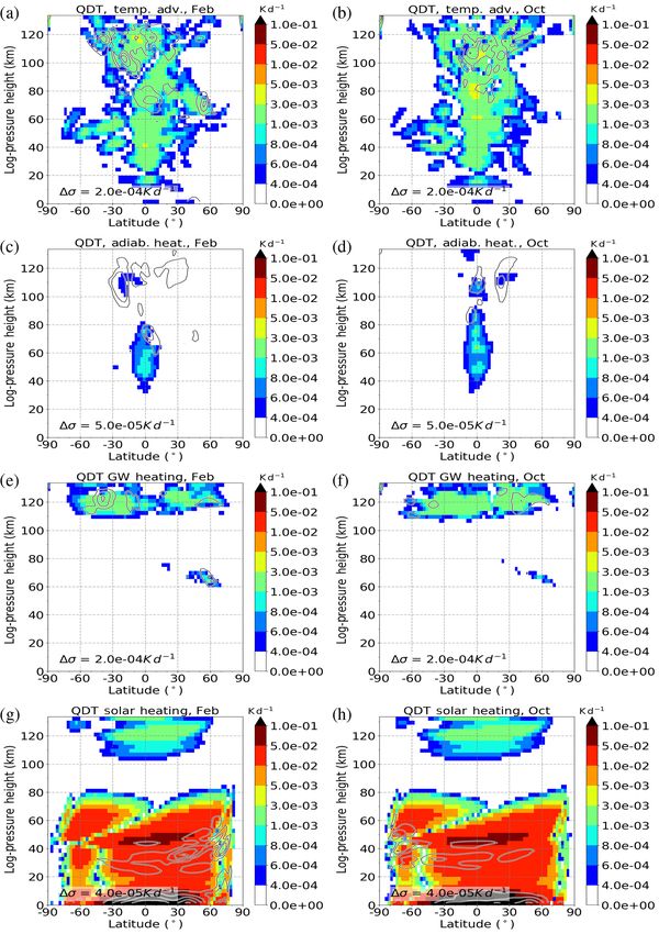
532                                            C. Geißler et al.: Forcing mechanisms of the migrating quarterdiurnal tide

mostly amounts to less than σ (T ) = 2 K (σ (u) = 2 ms−1 ,       are again scaled by exp[−z(2H )−1 ] according to energy con-
σ (v) = 0.5 ms−1 ).                                              servation. The different panels show the zonal (Fig. 4a, b)
   In comparison with the more recent Horizontal Wind            and meridional wind advection (Fig. 4c, d) as well as the
Model (HWM14; Drob et al., 2015), the westerly wind              zonal (Fig. 4e, f) and meridional (Fig. 4g, h) acceleration
jet in February in the middle atmosphere midlatitudes is         due to gravity waves. In the troposphere, stratosphere and
much stronger (+20 ms−1 ) in the MUAM simulation. The            large parts of the mesosphere, the nonlinear forcing of both
easterly wind jet in the mesosphere, in contrast, is much        the zonal (Fig. 4a, b) and meridional (Fig. 4c, d) QDT wind
weaker (−35 ms−1 ) in the MUAM simulation than predicted         dominates over the gravity wave forcing (Fig. 4e, f, g, h).
by HWM14. Furthermore, the mesospheric wind reversal             Near the mesopause, gravity wave zonal and meridional forc-
is found at higher altitudes in HWM14 (100 km) than in           ing is more important than the nonlinear forcing in zonal and
the MUAM (80 km) simulation, especially in the Northern          meridional wind. The zonal gravity wave forcing becomes
Hemisphere. Similarly, the wind jets in the mesopause and        relatively strong above 60 km at the northern middle lati-
lower thermosphere region are much weaker in the MUAM            tudes. The gravity wave forcing plays a major role above
run than in HWM14. Better agreement is seen for October          110 km, where it dominates over other nonlinear forcings.
regarding the strength of the wind jets. However, in contrast    In the meridional component, the wind advection (Fig. 4c, d)
to February, the wind reversal in October is higher in MUAM      outweighs the gravity wave forcing (Fig. 4g, h) at almost all
(80 km) than in HWM14 (70 km).                                   altitudes.
   All QDT forcing terms, including the solar forcing, non-
linear forcing and the forcing resulting from gravity wave–      3.2   Separation of quarterdiurnal generation
tide interactions, are shown in Fig. 3 (thermal parameters)            mechanisms
and Fig. 4 (wind parameters) for February (a, c, ,e ,g) and
October (b, d, f, h). All of these forcing terms in the MUAM     To quantify the effect of each forcing mechanism on the
tendency equations are scaled by the factor exp[−z(2H )−1 ]      QDT, we performed simulations with various forcing terms
in order to account for the growth rate of the amplitudes with   switched off (see Table 1). For the months of February and
altitude due to decreasing density. Thus, the figures show the   October, the QDT amplitudes and phases of the simulations
source regions of the QDT. However, from the parameters          REF, SOL, GW and NLIN are shown in Figs. 5–8 (Fig. 5a
shown in Figs. 3 and 4, no statement about the propagation       and b show temperature, and Fig. 7a and b show zonal wind).
conditions of the QDT is possible because the tide might be      Note that amplitudes are not scaled in contrast to the forcing
trapped in the source region and be unable to propagate up-      terms in Figs. 3 and 4. In October, the amplitudes tend to
wards (Lilienthal et al., 2018). In general, the QDT in situ     be a little stronger than in February (Fig. 5), and the ampli-
forcing in February and October shows a similar global dis-      tudes generally increase with height. In the REF run, there
tribution.                                                       are four maxima for temperature and zonal wind. At an al-
   Figure 3 shows temperature advection (Fig. 3a, b), the        titude of 100 km, amplitudes up to 0.5 K in temperature and
nonlinear component of adiabatic heating (Fig. 3c, d), the       1.5 ms−1 in zonal wind are achieved. Thus, the modeled am-
heating related to dissipating gravity waves (Fig. 3e, f), and   plitudes are much smaller than those reported from measure-
direct solar heating (Fig. 3g, h). Note the different color      ments (e.g., Liu et al., 2015; Azeem et al., 2016; Jacobi et al.,
scales in Fig. 3 to cover the maxima of all forcing terms. The   2017b; Guharay et al., 2018), i.e., satellite measurements re-
thermal forcing of the QDT is dominated by direct solar heat-    veal temperature amplitudes of 5–10 K, depending on season
ing in the troposphere and stratosphere (Fig. 3g, h). This is    and altitude, whereas radar data suggest wind amplitudes of
due to the absorption of solar radiation by water vapor in the   2.5–5 ms−1 .
troposphere and ozone in the stratosphere. In the mesosphere        In Fig. 5c and d, the SOL simulations for February and
(80–110 km) nonlinear wave–wave interactions (Fig. 3a, b)        October are shown for temperature; in Fig. 7c and d, they are
play the most important role and show maxima at the Equa-        shown for zonal wind. In this run, the gravity wave forcing
tor in the stratosphere, mesosphere and lower thermosphere.      mechanism and the nonlinear forcing mechanism were re-
Nonlinear adiabatic heating (Fig. 3c, d) maximizes in the up-    moved from the terms of the model tendency equation, as de-
per stratosphere and mesosphere at the Equator. However,         scribed in Sect. 2. The QDT amplitudes in the SOL run look
this forcing is about 1 order of magnitude smaller than the      very similar to those of the REF run in terms of amplitude
nonlinear forcing and, therefore, will be disregarded in the     magnitude and distribution. This agrees well with Fig. 3g
following. In the lower thermosphere, the strongest QDT          and h, showing that direct solar forcing is the strongest forc-
generation second to solar heating takes place through grav-     ing mechanism and dominates the QDT in situ generation.
ity wave heating (Fig. 3e, f). Nevertheless, nonlinear effects   On closer examination, the midlatitudes of both hemispheres
continue to occur, and they are partly comparable in magni-      show even larger temperature and zonal wind amplitudes
tude to the gravity wave forcing.                                in the SOL run than in the REF run, in particular during
   Figure 4 shows QDT acceleration terms in the momentum         February. Conversely, amplitudes during October tend to be
equations and, thus, refers to the wind parameters. The data     slightly decreased in the SOL simulation but with similar

Ann. Geophys., 38, 527–544, 2020                                                         www.ann-geophys.net/38/527/2020/
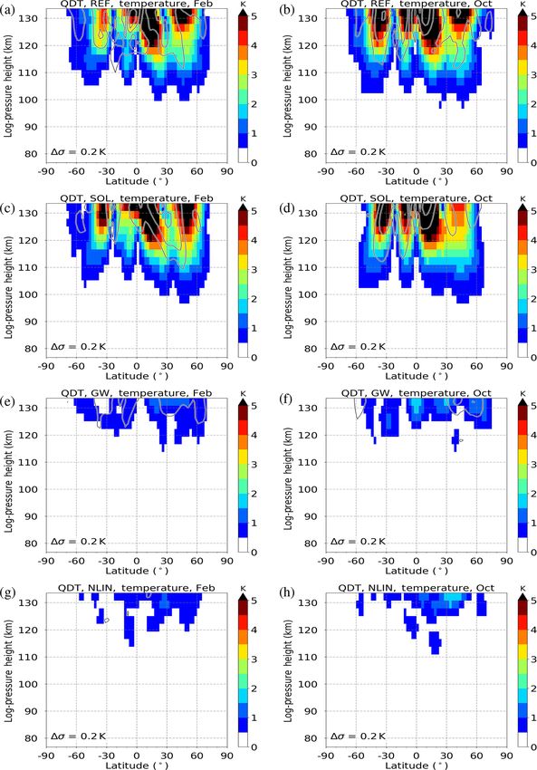
C. Geißler et al.: Forcing mechanisms of the migrating quarterdiurnal tide                                                           533

Figure 3. Quarterdiurnal component of thermal tendency terms in the REF simulation for February conditions (a, c, e, g) and October
conditions (b, d, f, h). Amplitudes are scaled by exp[−z(2H )−1 ]. Results are an average of the 11 ensemble members (shaded color).
Standard deviations (σ ) are added as gray contour lines. Panels (a) and (b) show temperature advection (nonlinear component), panels (c)
and (d) show adiabatic heating (nonlinear component), panels (e) and (f) show heating due to gravity wave activity (tendency term from
gravity wave parameterization), and panels (g) and (h) show solar heating (tendency term from solar radiation parameterization). Note that
the color scales are different and that the scale in panels (g) and (h) is not linear.

global structure to those of the REF simulation. The GW                are located at northern low latitudes of the lower thermo-
run only contains the gravity wave forcing and shows only              sphere; however, they are negligible below 115 km. This is
small amplitudes for the temperature (Fig. 5e, f; up to 2 K)           most likely due to the fact that gravity wave–tide interactions
and zonal wind (Fig. 7e, f; up to 3.5 ms−1 ) compared with             mainly take effect in the lower thermosphere (see Figs. 3 and
the REF and SOL simulations. Similar to the REF simula-                4).
tion, amplitudes gradually increase with height, and maxima

www.ann-geophys.net/38/527/2020/                                                                  Ann. Geophys., 38, 527–544, 2020
534                                                C. Geißler et al.: Forcing mechanisms of the migrating quarterdiurnal tide

Figure 4. Quarterdiurnal component of zonal and meridional wind acceleration terms in the REF simulation for February conditions (a, c, e,
g) and October conditions (b, d, f, h). Amplitudes are scaled by exp[−z(2H )−1 ]. Results are an average of the 11 ensemble members (shaded
color). Standard deviations (σ ) are added as gray contour lines. Panels (a) and (b) show the zonal wind advection (nonlinear component),
panels (c) and (d) show the meridional wind advection (nonlinear component), panels (e) and (f) show the zonal acceleration due to gravity
waves, and panels (h) and (h) show the meridional acceleration due to gravity waves (tendency terms from gravity wave parameterization).
Note that the color scales are different.

   Figures 5g and h and 7g and h show the QDT amplitudes                GW run with less than 1.5 ms−1 . Therefore, we cannot derive
for the NLIN run. This simulation contains only the forcing             a clear meridional structure of the nonlinear QDT. Keeping
of nonlinear interactions. The amplitudes for the tempera-              in mind that nonlinear tidal interactions mainly occur in the
ture component (Fig. 5g, h) are comparable to those of the              mesosphere (see Figs. 3 and 4), one may conclude that QDTs
GW run with a maximum of 2 K. For the zonal wind compo-                 generated by this mechanism are trapped near their forcing
nent (Fig. 7g, h), the amplitudes are even smaller than in the          region and cannot propagate further upward.

Ann. Geophys., 38, 527–544, 2020                                                                 www.ann-geophys.net/38/527/2020/
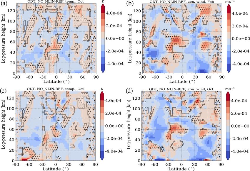
C. Geißler et al.: Forcing mechanisms of the migrating quarterdiurnal tide                                                        535

Figure 5. Simulations of zonal mean QDT amplitudes for temperature (colors), showing (a, c, e, g) February and (b, d, f, h) October
conditions. Panels (a) and (b) show the REF run with all forcing mechanisms enabled, panels (c) and (d) show the SOL run with only the
direct solar forcing mechanism enabled, panels (e) and (f) show the GW run with only the gravity wave forcing mechanism enabled, and
panels (g) and (h) show the NLIN run with only the nonlinear forcing mechanism enabled. Standard deviations σ are added as gray contour
lines.

   In addition, a NO_NLIN run was performed in which only             only interactions between tides and gravity waves removed
quarterdiurnal nonlinear interactions were removed. The am-           in the model tendency terms. The amplitudes (Figs. S1, S3)
plitudes of the NO_NLIN simulation are even larger than               and phases (Figs. S2, S4) of these simulations are shown in
those in the REF simulation. This fact is also seen for the           the Supplement, because amplitude and phase differences are
SOL simulations compared with the REF run. Larger ampli-              rather small compared with the REF simulation. Similar be-
tudes are also partly visible for the NO_GW simulation, with          havior has been reported by Smith et al. (2004), who removed

www.ann-geophys.net/38/527/2020/                                                                Ann. Geophys., 38, 527–544, 2020
536 C. Geißler et al.: Forcing mechanisms of the migrating quarterdiurnal tide
the nonlinear QDT forcing in their model and concluded that is expected to be larger than in REF, because the non-
tidal interactions reduced rather than enhanced the QDT am- linear (NLIN) and solar (SOL) QDT of the REF run act
plitude. In the following, this is investigated in more detail against each other. Indeed, we observe regions for temper-
by analyzing phase differences between the differently gen- ature (Fig. 9a, c) and zonal wind (Fig. 9b, d) in which the
erated QDTs. In this way, we intend to reveal possible inter- amplitudes in the NO_NLIN run are larger than in the REF
actions between these waves. simulation, and destructive interference between the nonlin-
The corresponding phases of the REF simulation can be ear and solar QDT concurrently corresponds to these posi-
found in Fig. 6a and b for temperature and in Fig. 8a and b for tive amplitude differences. Thus, we can conclude that the
zonal wind. The corresponding vertical wavelength can be nonlinearly excited part of the QDT weakens the pure solar
determined at any latitude from the vertical phase gradient. QDT amplitude in the REF simulation. The effect is more
The wavelength is defined by the vertical distance between pronounced for the zonal wind than for temperature.
two points with identical phases and should cover a com- In addition to the interaction between nonlinear and so-
plete span of phases. According to theory, an upward propa- lar QDT, an interaction between gravity-wave-induced QDT
gating wave must have a negative phase gradient. At latitudes and solar QDT is also possible. For this reason, we show the
with large amplitudes, the vertical wavelengths tend to also respective results in Fig. 10, which is comparable to Fig. 9.
be larger. In the opposite case, the wavelengths are smaller Colors denote the differences between the NO_GW and the
when the amplitudes are small. In February, the wavelengths REF simulation, which are again scaled by the growth rate of
reach 100 km or more. In October, phases are very similar. the amplitudes with altitude. Red (blue) colors denote larger
Both months show large areas with constant phases, espe- NO_GW (REF) amplitudes. Areas of destructive interference
cially at low latitudes. (see Eq. 1 with 18 = 8GW − 8SOL ) between the phases
Moreover, the QDT phases for the temperature (Fig. 6c, from the NO_GW and SOL run are hatched. The difference
d) and the zonal wind (Fig. 8c, d) component of the SOL between the NO_GW and the REF runs shows that the ampli-
simulation are almost identical to the results of the REF run. tudes in the NO_GW simulation are sometimes larger than in
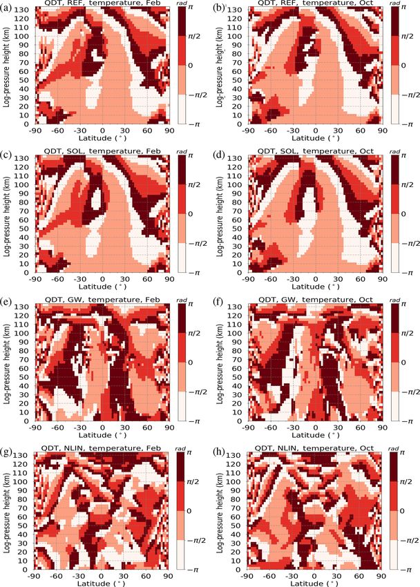
The phases of the GW run (Figs. 6d, f and 8d, f) clearly dif- the REF run. This often happens in areas where destructive
fer from the REF run, i.e., vertical wavelengths are shorter interference can be detected, but it is less well pronounced
and the phase position and distribution have also changed. than in Fig. 9 for the nonlinear–solar QDT interaction. This
Looking at the QDT phases of the NLIN run for temperature means that the QDT owing to gravity wave–tide interactions
(Fig. 6g, h) and zonal wind (Fig. 8g, h), the associated ver- also tends to act against the solar QDT which leads to a de-
tical wavelengths are again smaller compared with the GW cline in QDT amplitude in the REF simulation for temper-
run, based on a more irregular phase distribution. ature and zonal wind, where both forcing mechanisms are
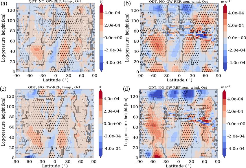
In Fig. 9, we present QDT amplitude differences be- present. The interaction between GW and NLIN QDT is not
tween the NO_NLIN and REF simulations, which are scaled shown separately because they were found to be negligible.
by density to highlight the actual source region of the
waves. Here, the red (blue) areas denote larger amplitudes
in NO_NLIN (REF) simulations. This means that the run 4 Discussion and conclusion
with one forcing removed has larger amplitudes than the REF
run in red areas. We conclude that the removed nonlinear The results of the REF simulation show a consensus in the
forcing must have destructively interfered with other QDT climatology and global structure of QDT in comparison with
from other forcings (such as solar or gravity wave forcing). observations and other model studies. The amplitudes of the
The NLIN run (only nonlinear forcing) is expected to show MUAM are relatively small for the QDT with up to 2.5 ms−1
small QDT amplitudes because of the weak nonlinear forc- in the zonal wind at an altitude of 101 km and 5.0 ms−1 at an
ing. Without destructive interference, the NO_NLIN (with- altitude of 120 km in spring and autumn. For example, QDT
out nonlinear forcing) simulation should show larger ampli- amplitudes obtained from meteor radar measurements (Ja-
tudes than the NLIN run but smaller amplitudes than the REF cobi et al., 2017b) are up to 3 times larger than in the MUAM
run, because one forcing (nonlinear) is missing. Figure 9a simulations. However, it is a known issue that numerical
and c show the temperature component, and Fig. 9b and d models tend to underestimate the tides in some regions and
show the zonal wind component in February and October, re- seasons (e.g., Smith, 2012; Pokhotelov et al., 2018).
spectively. Furthermore, the hatched areas denote destructive In our simulations, the meridional structure of QDT ampli-
interference between the QDTs of NLIN and SOL, which are tudes shows three to four maxima in both the temperature and
defined by their phases differences 18 = 8NLIN − 8SOL : zonal wind component. These are located at low (10–30◦ )
and middle latitudes (40–70◦ ) of the respective hemisphere.
120◦ ≤ 18 ≤ 240◦ . (1) These maxima at low and midlatitudes are also present in
the NIRS and SABER temperature measurements (Liu et al.,
In the case of a superposition of such destructively re- 2015; Azeem et al., 2016). Meteor radar measurements at
lated NLIN and SOL waves, the amplitude of NO_NLIN northern midlatitudes (Jacobi et al., 2017b) confirm our QDT
Ann. Geophys., 38, 527–544, 2020 www.ann-geophys.net/38/527/2020/C. Geißler et al.: Forcing mechanisms of the migrating quarterdiurnal tide 537 Figure 6. Simulations of zonal mean QDT phases for temperature (colors), showing (a, c, e, g) February and (b, d, f, h) October conditions. Panels (a) and (b) show the REF run with all forcing mechanisms enabled, panels (c) and (d) show the SOL run with only the direct solar forcing mechanism enabled, panels (e) and (f) show the GW run with only the gravity wave forcing mechanism enabled, and panels (g) and (h) show the NLIN run with only the nonlinear forcing mechanism enabled. Standard deviations σ are added as gray contour lines. wind maxima in winter, spring and autumn. The maximum of proach of Lilienthal et al. (2018). These are (i) the absorption the QDT wind amplitudes at low latitudes has been proven of solar radiation by water vapor and ozone, (ii) nonlinear by meteor radar measurements over Brazil (Guharay et al., tidal interactions between migrating DTs and TDTs and the 2018). They show maxima below 100 km in spring and au- self-interaction of migrating SDTs, and (iii) nonlinear inter- tumn as in the MUAM simulations. actions between gravity waves and tides. To our knowledge, In the present paper, we focused on forcing mechanisms of this is the first time that the global distribution of quarterdi- the QDT. To this end, we first compared all possible sources urnal in situ forcing from a numerical model has been pre- of the migrating QDTs in our simulations following the ap- sented. In summary, the solar forcing dominates in the tropo- www.ann-geophys.net/38/527/2020/ Ann. Geophys., 38, 527–544, 2020
538                                              C. Geißler et al.: Forcing mechanisms of the migrating quarterdiurnal tide

Figure 7. Same as Fig. 5 but for QDT zonal wind amplitudes.

sphere and stratosphere, the nonlinear forcing predominates       anism remains and the other two sources are removed (SOL,
in the mesosphere, and the gravity wave forcing mainly takes      NLIN and GW), whereas in other simulations only one of the
place in the mesosphere and thermosphere. These results do        sources was removed (NO_NLIN and NO_GW).
not allow us to draw conclusions on the upward propagation           As a result, we find that the solar forcing mechanism is
of the QDT, as they only show local excitation.                   the most important and dominant of all forcing mechanisms,
   For this reason, we adapt the idea of Smith et al. (2004),     as the removal of direct quarterdiurnal solar heating (GW and
who performed simulations with individual forcing mecha-          NLIN runs) leads to a significant decrease in the QDT ampli-
nisms removed. In addition to Smith et al. (2004), we also        tude. Smith et al. (2004) came to the same conclusion when
consider gravity wave–tide interactions. Some of our simula-      they removed the quarterdiurnal solar forcing in their simu-
tions are designed in a way that only a single forcing mech-      lations.

Ann. Geophys., 38, 527–544, 2020                                                         www.ann-geophys.net/38/527/2020/
C. Geißler et al.: Forcing mechanisms of the migrating quarterdiurnal tide                                                  539

Figure 8. Same as Fig. 6 but for QDT zonal wind phases.

   We also showed that the amplitudes resulting from the        domain. Significant nonlinear QDT amplitudes only exist in
gravity wave forcing mechanism (GW) are smaller than the        the thermosphere. In the temperature component, QDT am-
resulting amplitudes of the direct solar forcing (SOL), but     plitudes of the NLIN and GW simulations are comparable in
they are larger than those from the nonlinear forcing mecha-    magnitude. In the zonal wind component, they are smaller
nisms (NLIN). In agreement with the results of Smith et al.     in NLIN than in GW. For the GW and NLIN simulations,
(2004), nonlinear tidal interactions seem to play a minor       we note relatively short vertical wavelengths, accompanied
role in the total QDT amplitudes, although we found distinct    by small QDT amplitudes, compared with the SOL and REF
sources of nonlinear quarterdiurnal in situ excitation in the   runs. Therefore, we can state that if the amplitudes are small,
mesosphere (see above). This allows for the conclusion that     the vertical wavelength is also shorter. Lilienthal et al. (2018)
the QDT from local nonlinear forcing mechanisms can not         found a similar relation for the vertical wavelengths of the
propagate and is, to a large degree, trapped in the vertical    TDT.

www.ann-geophys.net/38/527/2020/                                                          Ann. Geophys., 38, 527–544, 2020
540                                              C. Geißler et al.: Forcing mechanisms of the migrating quarterdiurnal tide

Figure 9. Difference of QDT amplitudes between NO_NLIN and REF simulation, scaled by exp[−z(2H )−1 ]. Red denotes larger NO_NLIN
simulation amplitudes, and blue denotes larger REF simulation amplitudes. Areas of destructive interference (120◦ ≤ 18 ≤ 240◦ ) between
NLIN and SOL phases are hatched. Panels (a) and (c) show temperature, and panels (b) and (d) show zonal wind for (a, b) February
conditions and (c, d) October conditions.

Figure 10. Difference of QDT amplitudes between the NO_GW and REF simulations, scaled by exp[−z(2H )−1 ]. Red denotes larger
NO_GW simulation amplitudes, and blue denote larger REF simulation amplitudes. Areas of destructive interference (120◦ ≤ 18 ≤ 240◦ )
between the GW and SOL phases are hatched. Panels (a) and (c) show temperature, and panels (b) and (d) show zonal wind for (a, b)
February and (c, d) October conditions.

Ann. Geophys., 38, 527–544, 2020                                                               www.ann-geophys.net/38/527/2020/
C. Geißler et al.: Forcing mechanisms of the migrating quarterdiurnal tide                                                             541

   In the SOL simulation, which only contains the solar forc-         Author contributions. CG and FL performed and designed the
ing, we see that the amplitudes are larger than in the REF run        MUAM model runs. CG drafted the first version of the text. The
in some cases. A similar feature was observed by Smith et al.         analysis and interpretation of the results were contributed by CJ and
(2004). Here, we compare phase and amplitude differences              FL.
between our different simulations to investigate the physi-
cal explanation behind this. We find that the amplitudes in
simulations with removed forcing mechanisms (NO_NLIN                  Competing interests. Christoph Jacobi is one of the editors in chief
                                                                      of Annales Geophysicae. The authors declare that no competing in-
and NO_GW) increase compared with the REF simulation
                                                                      terests are present.
in the same areas where destructive phase relations between
the differently generated QDTs are detected. This leads to
the conclusion that QDTs that are excited by different mech-          Acknowledgements. This research has been funded by the
anisms counteract rather than enhance each other. Therefore,          Deutsche Forschungsgemeinschaft (under grant no. JA 836/34-
removing an individual forcing mechanism in NO_NLIN or                1). MERRA-2 global ozone fields were provided by NASA
NO_GW also avoids the destructive interference, and the re-           at     https://disc.gsfc.nasa.gov/datasets?keywords="MERRA-2"&
maining QDT can propagate freely, resulting in larger ampli-          page=1&source=Models%2FAnalysesMERRA-2, last access:
tudes.                                                                16 April 2020 (MERRA-2, 2019; Gelaro et al., 2017). Mauna
   This destructive relation appears to be more clear between         Loa carbon dioxide mixing ratios were provided by NOAA at
the nonlinear tidal forcing and the direct solar forcing than         ftp://aftp.cmdl.noaa.gov/products/trends/co2/co2_mm_mlo.txt,
between the gravity wave-induced forcing and the solar forc-          last access: 16 April 2020 (Thoning et al., 1989; NOAA
ing. Note, however, that nonlinear tidal interactions generally       ESRL Global Monitoring Division, 2018). ERA-Interim
                                                                      data were provided by ECMWF at https://apps.ecmwf.
have a smaller impact on the QDT than gravity wave–tide in-
                                                                      int/datasets/data/interim-full-moda/levtype=sfc/,     last   ac-
teractions, as described above. We do not present phase re-
                                                                      cess: 16 April 2020 (Dee et al., 2011; ERA-Interim,
lations between the nonlinear and gravity wave forcing be-            2018). GSWM tides data were provided by HAO at
cause these were found to be small. Apparently, the dominat-          https://www2.hao.ucar.edu/gswm-global-scale-wave-model,
ing solar forcing has to be involved in the destructive phase         last access: 16 April 2020 (Hagan et al., 1999).
relation. In future, an implementation of a latent heat release
parameterization according to Ermakova et al. (2019) and Ja-
cobi et al. (2017a) and 3-D ozone (Suvorova and Pogoreltsev,          Financial support. This research has been supported by the
2011) and water vapor (Ermakova et al., 2017) fields into             Deutsche Forschungsgemeinschaft (grant no. JA 836/34-1).
the model is planned, which may help to increase tidal am-
plitudes towards more realistic magnitudes. Another impor-
tant issue is the careful treatment of gravity waves, because         Review statement. This paper was edited by Andrew J. Kavanagh
we demonstrated that gravity waves are the most important             and reviewed by two anonymous referees.
source of QDTs above the mesopause. In MUAM, gravity
waves are currently implemented via two coupled parame-
terizations. These two parameterizations could be replaced
by the original whole atmosphere scheme, as provided by
                                                                      References
Yiğit et al. (2008). Furthermore, a sensitivity study with re-
spect to the strength of the individual forcing terms may con-
                                                                      Andrews, D. G., Leovy, C. B., and Holton, J. R.: Middle atmosphere
tribute to a better understanding of the forcing mechanisms             dynamics, vol. 40, Academic press, 1987.
and interactions, thereby showing their impact on QDT am-             Azeem, I., Walterscheid, R. L., Crowley, G., Bishop, R. L.,
plitudes and the background circulation. Further examination            and Christensen, A. B.: Observations of the migrating semid-
of dominating Hough modes may help explain the different                iurnal and quaddiurnal tides from the RAIDS/NIRS in-
meridional structures at different altitudes.                           strument, J. Geophy. Res.-Space Phys., 121, 4626–4637,
                                                                        https://doi.org/10.1002/2015JA022240, 2016.
                                                                      Chapman, S. and Lindzen, R. S.: Atmospheric Tides, D. Reidel Pub-
Code availability. The MUAM model code can be obtained from             lishing Company (Dordrecht, Holland), 1970.
the corresponding author upon request.                                Dee, D. P., Uppala, S. M., Simmons, A. J., Berrisford, P., Poli,
                                                                        P., Kobayashi, S., Andrae, U., Balmaseda, M. A., Balsamo, G.,
                                                                        Bauer, P., Bechtold, P., Beljaars, A. C. M., van de Berg, L., Bid-
Supplement. The supplement related to this article is available on-     lot, J., Bormann, N., Delsol, C., Dragani, R., Fuentes, M., Geer,
line at: https://doi.org/10.5194/angeo-38-527-2020-supplement.          A. J., Haimberger, L., Healy, S. B., Hersbach, H., Hólm, E. V.,
                                                                        Isaksen, L., Kållberg, P., Köhler, M., Matricardi, M., McNally,
                                                                        A. P., Monge-Sanz, B. M., Morcrette, J.-J., Park, B.-K., Peubey,
                                                                        C., de Rosnay, P., Tavolato, C., Thépaut, J.-N., and Vitart, F.: The
                                                                        ERA-Interim reanalysis: configuration and performance of the

www.ann-geophys.net/38/527/2020/                                                                  Ann. Geophys., 38, 527–544, 2020
542 C. Geißler et al.: Forcing mechanisms of the migrating quarterdiurnal tide data assimilation system, Q. J. Roy. Meteor. Soc., 137, 553–597, GSWM: Amplitudes and phases of the diurnal and semidiur- https://doi.org/10.1002/qj.828, 2011. nal migirating tides from Global Scale Wave Modela available Drob, D. P., Emmert, J. T., Meriwether, J. W., Makela, J. J., at: https://www2.hao.ucar.edu/gswm-global-scale-wave-model Doornbos, E., Conde, M., Hernandez, G., Noto, J., Zawdie, (last acess: 2 March 2020), 2020. K. A., McDonald, S. E., Huba, J. D., and Klenzing, J. H.: Guharay, A., Batista, P. P., Buriti, R. A., and Schuch, N. J.: An update to the Horizontal Wind Model (HWM): The On the variability of the quarter-diurnal tide in the MLT over quiet time thermosphere, Earth and Space Sci., 2, 301–319, Brazilian low-latitude stations, Earth Planet. Space, 70, 140, https://doi.org/10.1002/2014EA000089, 2015. https://doi.org/10.1186/s40623-018-0910-9, 2018. ERA-Interim: Monthly mean temperature and geopotential fields on Hagan, M. E., Forbes, J. M., and Vial, F.: On modeling pressure levels 1979-date; Eurpoean Reanalysis Interim, avail- migrating solar tides, Geophys. Res. Lett., 22, 893–896, able at: https://apps.ecmwf.int/datasets/data/interim-full-moda/ https://doi.org/10.1029/95GL00783, 1995. levtype=pl/, compiled by Thoning, K. W., Kitzis, D. R., and Hagan, M. E., Burrage, M. D., Forbes, J. M., Hackney, J., Crotwell, A., Version 2015-12, updated annually, 2018. Randel, W. J., and Zhang, X.: GSWM-98: Results for mi- Ermakova, T. S., Statnaya, I. A., Fedulina, I. N., Suvorova, grating solar tides, J. Geophys. Res.-Space, 104, 6813–6827, E. V., and Pogoreltsev, A. I.: Three-dimensional semi-empirical https://doi.org/10.1029/1998JA900125, 1999. climate model of water vapor distribution and its imple- Jacobi, C., Portnyagin, Y., Solovjova, T., Hoffmann, P., Singer, mentation to the radiation module of the middle and up- W., Fahrutdinova, A., Ishmuratov, R., Beard, A., Mitchell, N., per atmosphere model, Russ. Meteorol. Hydrol., 42, 594–600, Muller, H., Schminder, R., Kürschner, D., Manson, A., and https://doi.org/10.3103/S1068373917090060, 2017. Meek, C.: Climatology of the semidiurnal tide at 52–56◦ N from Ermakova, T. S., Aniskina, O. G., Statnaia, I. A., Motsakov, M. A., ground-based radar wind measurements 1985–1995, J. Atmos. and Pogoreltsev, A. I.: Simulation of the ENSO influence on Sol.-Terr. Phys., 61, 975–991, https://doi.org/10.1016/S1364- the extra-tropical middle atmosphere, Earth Planet. Space, 71, 6826(99)00065-6, 1999. 8, https://doi.org/10.1186/s40623-019-0987-9, 2019. Jacobi, C., Fröhlich, K., and Pogoreltsev, A.: Quasi two- Fleming, E. L., Chandra, S., Barnett, J., and Corney, M.: day-wave modulation of gravity wave flux and conse- Zonal mean temperature, pressure, zonal wind and geopoten- quences for the planetary wave propagation in a simple cir- tial height as functions of latitude, Adv. Space Res., 10, 11–59, culation model, J. Atmos. Sol.-Terr. Phys., 68, 283–292, https://doi.org/10.1016/0273-1177(90)90386-E, 1990. https://doi.org/10.1016/j.jastp.2005.01.017, 2006. Forbes, J., Manson, A., Vincent, R., Fraser, G., Vial, F., Wand, Jacobi, C., Fröhlich, K., Portnyagin, Y., Merzlyakov, E., Solovjova, R., Avery, S., Clark, R., Johnson, R., Roper, R., Schminder, T., Makarov, N., Rees, D., Fahrutdinova, A., Guryanov, V., Fe- R., Tsuda, T., and Kazimirovsky, E.: Semidiurnal tide in the dorov, D., Korotyshkin, D., Forbes, J., Pogoreltsev, A., and 80–150 km region: an assimilative data analysis, J. Atmos. Kürschner, D.: Semi-empirical model of middle atmosphere Sol.-Terr. Phys., 56, 1237–1249, https://doi.org/10.1016/0021- wind from the ground to the lower thermosphere, Adv. Space 9169(94)90062-0, 1994. Res., 43, 239–246, https://doi.org/10.1016/j.asr.2008.05.011, Forbes, J. M.: Atmospheric tides: 1. Model description and results 2009. for the solar diurnal component, J. Geophy. Res.-Space Phys., 87, Jacobi, C., Ermakova, T., Mewes, D., and Pogoreltsev, A. I.: 5222–5240, https://doi.org/10.1029/JA087iA07p05222, 1982a. El Niño influence on the mesosphere/lower thermosphere cir- Forbes, J. M.: Atmospheric tide: 2. The solar and lunar semidiur- culation at midlatitudes as seen by a VHF meteor radar nal components, J. Geophy. Res.-Space Phys., 87, 5241–5252, at Collm (51.3◦ N, 13◦ E), Adv. Radio Sci., 15, 199–206, https://doi.org/10.1029/JA087iA07p05241, 1982b. https://doi.org/10.5194/ars-15-199-2017, 2017a. Fröhlich, K., Pogoreltsev, A., and Jacobi, C.: The 48 Layer Jacobi, C., Krug, A., and Merzlyakov, E.: Radar observa- COMMA-LIM Model: Model description, new Aspects, tions of the quarterdiurnal tide at midlatitudes: Seasonal and and Climatology, Rep. Inst. Meteorol. Univ. Leipzig, pp. long-term variations, J. Atmos. Sol.-Terr. Phys., 163, 70–77, 161–189, available at: http://nbn-resolving.de/urn:nbn:de:bsz: https://doi.org/10.1016/j.jastp.2017.05.014, 2017b. 15-qucosa-217766 (last access: 16 April 2020), 2003a. Jacobi, C., Geißler, C., Lilienthal, F., and Krug, A.: Forcing mech- Fröhlich, K., Pogoreltsev, A., and Jacobi, C.: Numerical anisms of the 6 h tide in the mesosphere/lower thermosphere, simulation of tides, Rossby and Kelvin waves with the Adv. Radio Sci., 16, 141–147, https://doi.org/10.5194/ars-16- COMMA-LIM model, Adv. Space Res., 32, 863–868, 141-2018, 2018. https://doi.org/10.1016/S0273-1177(03)00416-2, 2003b. Jacobi, C., Arras, C., Geißler, C., and Lilienthal, F.: Quarterdi- Gelaro, R., McCarty, W., Suárez, M. J., Todling, R., Molod, A., urnal signature in sporadic E occurrence rates and compar- Takacs, L., Randles, C. A., Darmenov, A., Bosilovich, M. G., Re- ison with neutral wind shear, Ann. Geophys., 37, 273–288, ichle, R., Wargan, K., Coy, L., Cullather, R., Draper, C., Akella, https://doi.org/10.5194/angeo-37-273-2019, 2019. S., Buchard, V., Conaty, A., da Silva, A. M., Gu, W., Kim, G.- Jakobs, H., Bischof, M., Ebel, A., and Speth, P.: Simulation of grav- K., Koster, R., Lucchesi, R., Merkova, D., Nielsen, J. E., Par- ity wave effects under solstice conditions using a 3-D circula- tyka, G., Pawson, S., Putman, W., Rienecker, M., Schubert, S. D., tion model of the middle atmosphere, J. Atmos. Sol.-Terr. Phys., Sienkiewicz, M., and Zhao, B.: The Modern-Era Retrospective 48, 1203–1223, https://doi.org/10.1016/0021-9169(86)90040-1, Analysis for Research and Applications, Version 2 (MERRA-2), 1986. J. Climate, 30, 5419–5454, https://doi.org/10.1175/JCLI-D-16- Lilienthal, F. and Jacobi, C.: Nonlinear forcing mechanisms 0758.1, 2017. of the migrating terdiurnal solar tide and their impact on Ann. Geophys., 38, 527–544, 2020 www.ann-geophys.net/38/527/2020/
You can also read