Modeling the ice-attenuated waves in the Great Lakes - NOAA ...
←
→
Page content transcription
If your browser does not render page correctly, please read the page content below
Ocean Dynamics (2020) 70:991–1003
https://doi.org/10.1007/s10236-020-01379-z

Modeling the ice-attenuated waves in the Great Lakes
Peng Bai 1,2 & Jia Wang 2 & Philip Chu 2 & Nathan Hawley 2 & Ayumi Fujisaki-Manome 3,4 & James Kessler 2 &
Brent M. Lofgren 2 & Dmitry Beletsky 3 & Eric J. Anderson 2 & Yaru Li 3

Received: 12 January 2020 / Accepted: 23 April 2020 / Published online: 29 May 2020
# Springer-Verlag GmbH Germany, part of Springer Nature 2020

Abstract
A partly coupled wave-ice model with the ability to resolve ice-induced attenuation on waves was developed using the Finite-
Volume Community Ocean Model (FVCOM) framework and applied to the Great Lakes. Seven simple, flexible, and efficient
parameterization schemes originating from the WAVEWATCH III® IC4 were used to quantify the wave energy loss during wave
propagation under ice. The reductions of wind energy input and wave energy dissipation via whitecapping and breaking due to
presence of ice were also implemented (i.e., blocking effect). The model showed satisfactory performance when validated by buoy-
observed significant wave height in ice-free season at eight stations and satellite-retrieved ice concentration. The simulation ran over
the basin-scale, five-lake computational grid provided a whole map of ice-induced wave attenuation in the heavy-ice year 2014,
suggesting that except Lake Ontario and central Lake Michigan, lake ice almost completely inhibited waves in the Great Lakes
under heavy-ice condition. A practical application of the model in February 2011 revealed that the model could accurately reproduce
the ice-attenuated waves when validated by wave observations from bottom-moored acoustic wave and current profiler (AWAC);
moreover, the AWAC wave data showed quick responses between waves and ice, suggesting a sensitive relationship between
waves and ice and arguing that accurate ice modeling was necessary for quantifying wave-ice interaction.

Keywords Great Lakes . Wave dynamics . Ice-induced wave attenuation . FVCOM–SWAVE–UG-CICE

1 Introduction                                                                watershed. With large dimensions in addition to complex ge-
                                                                              ometry and topography, the Great Lakes present sea-like hy-
Extending approximately from 76.0 ° W to 92.1 ° W in longi-                   drodynamics under sustained atmospheric forcing (Beletsky
tude and 41.4 ° N to 49.0 ° N in latitude, the Laurentian Great               et al. 1999; Schwab and Beletsky 2003; Wang et al. 2012;
Lakes (Great Lakes) are the largest group of fresh water lakes                Bai et al. 2013).
on the Earth (Fig. 1a). The Great Lakes comprise about 1/5 of                    Genesis and melting of ice on the Great Lakes directly
the world’s surface freshwater, and nearly 1/8 of the American                modify the hydrodynamic processes, the thermal structure,
population and 1/3 of the Canadian population live within their               and the adjacent atmospheric boundary layer, mainly through
                                                                              three physical mechanisms: weakening surface wind stress;
This article is part of the Topical Collection on the 11th International      generating higher albedo than over open waters; and modify-
Workshop on Modeling the Ocean (IWMO), Wuxi, China, 17-20 June 2019           ing heat and moisture exchange processes between lake and
Responsible Editor: Tal Ezer                                                  atmosphere (Xue et al. 2017), which, in turn, affects the lake
                                                                              ecosystem (Vanderploeg et al. 1992; Brown et al. 1993), econ-
* Peng Bai                                                                    omy (Niimi 1982), and water level variability (Sellinger et al.
  peng.bai@noaa.gov; baip@gdou.edu.cn                                         2007). Lake ice coverage is characterized by large interannual
                                                                              variability (Fig. 1b) and is sensitive to the modulation of
1
    College of Ocean and Meteorology, Guangdong Ocean University,             teleconnection patterns such as the Arctic Oscillation and the
    Zhanjiang 524088, Guangdong, China                                        El Niño-Southern Oscillation (Wang et al. 2012; Bai et al.
2
    Great Lakes Environmental Research Laboratory, NOAA, Ann                  2012, 2015). Lake ice also plays a vital role in regional cli-
    Arbor, MI 48108, USA                                                      mate, for example, modulating the lake-effect snowfall
3
    Cooperative Institute for Great Lakes Research, University of             (Wright et al. 2013; Vavrus et al. 2013).
    Michigan, Ann Arbor, MI 48108, USA                                           Forced by winds, surface gravity waves generated on the
4
    Department of Climate and Space Sciences and Engineering,                 Great Lakes become one of the dominant driving forces for
    University of Michigan, Ann Arbor, MI 48104, USA                          lake hydrodynamics (Hubertz et al. 1991; Niu and Xia 2016;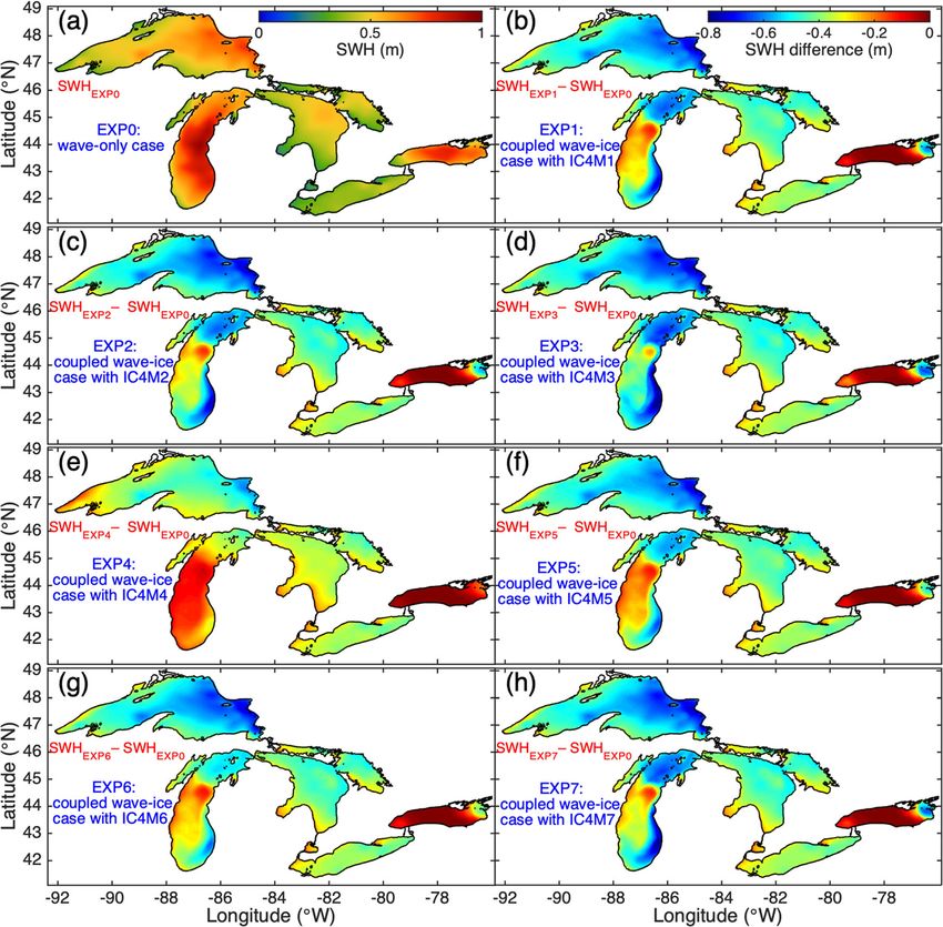
992                                                                                                       Ocean Dynamics (2020) 70:991–1003

Fig. 1 Topography and FVCOM computational meshes for the Great Lakes (a), red triangles show locations of the NDBC buoys. Great Lakes annual
maximum ice coverage from 1973 to 2019 (b). AWAC mooring locations (purple squares) in Lake Erie (c)

Mao and Xia 2017). Waves can interact with currents, leading            wave-enhanced surface stress can significantly modulate the
to stronger bottom shear stress, enhancing the vertical mixing          surges, offshore currents, and thermal structures.
and supplying additional momentum flux to the mean circu-                  During the ice season, lake waves generated in the open
lation. Conversely, in addition to exerting refraction, modifi-         waters can penetrate into the ice-covered region, causing in-
cation of bottom stress, and blocking effects on the waves              teraction between waves and ice. Part of the wave energy is
(Vincent 1979; Ris et al. 1999; Ardhuin et al. 2012), currents          reflected at the waterward periphery of the ice, and the remain-
could also change the wave frequency through Doppler shift;             ing energy, together with the winds and currents, would act on
meanwhile, variations in the water level could change the               the ice mechanically, modifying the growth process and hence
water depth felt by the waves (Pleskachevsky et al. 2009).              the morphology and structure of the ice cover, weakening and
Lake waves and lake circulation form a complicated                      rupturing the ice (Squire 2007; Barber et al. 2009; Vaughan
feedback system. For example, Brissette et al. (1993) revealed          and Squire 2011; Dumont et al. 2011; Williams et al. 2013;
that current-induced refraction can lead to significant differ-         Kohout et al. 2016). On the other hand, ice modulates the
ence between the wind and wave directions in Lake St. Clair.            waves mainly through three physical mechanisms: (1) attenu-
Wave-current interaction is found to play a critical role in            ation owing to the energy transfer and dissipation during
sediment resuspension and transport processes in Lake                   wave-ice interaction; (2) scattering caused by energy reflec-
Michigan by modifying the bottom shear stress (Lou et al.               tion at the ice edge; and (3) refraction due to different disper-
2000). Bai et al. (2013) suggested that wave mixing is a key            sion relations in the open seas and the ice-covered waters.
dynamical driver for lake thermal structure. Numerical inves-           Observations show that ice is often heterogeneous in nature
tigation by Niu and Xia (2017) indicated that, in Lake Erie,            and varied in form, which strongly impacts wave-ice
Ocean Dynamics (2020) 70:991–1003                                                                                                        993

interaction (e.g., Campbell et al. 2014). Wave propagation in         where N stands for the wave action density spectrum, t represents
ice is extensively investigated by employing various scatter-                   *                                  *
                                                                      the time, cg is the wave group velocity, U is the ambient flow
ing or viscous models. In scattering models, wave energy is           velocity vector, σ and θ are the intrinsic frequency and wave
reduced by accumulations of the partial energy reflections            direction, Cσ and Cθ are the wave propagation velocities in spec-
occurring when waves encounter a floe edge, and therefore,            tral space (σ, θ), Sin is the wind energy input, Snl is the energy
scattering models depend strongly on the distance waves trav-         transfer due to nonlinear wave-wave interactions among spectral
eling into the ice-covered waters and the distribution of ice         components, and Sds is the wave decay through wave breaking
floe size (Kohout and Meylan 2008; Bennetts and Squire                (Sds, br), whitecapping (Sds, w), and bottom friction (Sds, b).
2009; Bennetts and Squire 2011; Williams et al. 2013). In                 Presence of ice would inhibit the energy input by winds
viscous models, wave energy is decreased by viscous dissipa-          and restrain the wave energy decay via whitecapping and
tion, and hence, these models are independent of the floe size        breaking; therefore, these three source-sink terms are scaled
(Wang and Shen 2011; De Santi et al. 2018).                           by the open water fraction (hereinafter, the blocking effect).
    Understanding the wave-ice-lake interrelations is necessary       Meanwhile, the terms associated with the nonlinear wave-
for guiding proper navigation, engineering, hazard warning,           wave interactions and bottom friction remain the same as that
and regulatory actions in the Great Lakes. Previous investiga-        in open waters. Hence, wave propagation through ice-covered
tions have explored and emphasized the vital roles of wave-           waters is governed by:
lake interactions in the Great Lakes (e.g., Niu and Xia 2017;                     " * *! #
Mao and Xia 2017). However, we still have poor knowledge              ∂N                                ∂C σ N ∂C θ N
about how waves and ice interact with each other in the Great              þ∇        cg þ U N þ                 þ
                                                                       ∂t                                  ∂σ        ∂θ
Lakes. In this paper, we developed a partly coupled wave-ice

interaction model that able to describe the ice-induced wave                 ð1−C ice Þ S in þ S ds;w þ S ds;br þ S nl þ S ds;b þ S ice
attenuation within the Finite Volume Community Ocean                     ¼                                                              ; ð2Þ
                                                                                                         σ
Model (FVCOM) framework, and then we applied the model
to the Great Lakes.                                                   where Cice is the ice concentration, Sice = − αECg is a new
    The outline of the paper is as follows. Section 2 describes the   wave energy sink term due to the damping of ice cover, in
model, parameterization schemes quantifying ice-induced wave          which α is attenuation coefficient, E is wave spectral density,
attenuation, model configuration, numerical experiments, and          and Cg is wave group velocity.
observational data; in Sect. 3, a modeling estimation of ice-            The FVCOM includes an internally coupled ice model, the
induced wave attenuation in the Great Lakes during heavy-ice          UG-CICE, which was employed in this study to simulate the
year 2014 is presented; in Sect. 4, a practical application of the    lake ice dynamics. UG-CICE is an unstructured-grid, finite-
coupled wave-ice-lake model in February 2011 is demonstrated;         volume version of the Los Alamos Community Ice Code
and in Sect. 5, the major conclusions are summarized.                 (CICE, Hunke et al. 2010) implemented into the FVCOM
                                                                      framework by Gao et al. (2011); it employs the same governing
                                                                      equations as the CICE, has been widely applied to many cold
2 Data and methodology                                                regions including the Great Lakes, and showed satisfactory
                                                                      performance (e.g., Gao et al. 2011; Fujisaki-Manome and
2.1 FVCOM–SWAVE–UG-CICE                                               Wang 2016; Zhang et al. 2016; Anderson et al. 2018).

We used FVCOM (Chen et al. 2003), which is capable of re-             2.2 Parameterizing schemes for estimating
solving the complex topography in the Great Lakes, to model the       attenuation coefficient α
lake waves (FVCOM-SWAVE, Qi et al. 2009) and ice (UG-
CICE, Gao et al. 2011). FVCOM-SWAVE is a finite-volume                Many efforts have been dedicated to quantifying ice-induced
unstructured-grid third-generation wave model evolved from the        attenuation coefficient, i.e., α (e.g., Wadhams et al. 1988;
Simulating WAves Nearshore (SWAN, Booij et al. 1999), which           Kohout et al. 2007, 2014; Kohout and Meylan 2008;
models the wave generation, propagation, dissipation, refraction,     Meylan et al. 2014; Doble et al. 2015; Rogers et al. 2016).
and nonlinear wave-wave interactions by solving the wave action       However, some of the proposed theories are based on a
balance equation expressed as:                                        fluid-solid interactive frame, and the solving processes
           " * *! #                                                   are complicated and inefficient and therefore are diffi-
∂N                              ∂C σ N ∂C θ N                         cult to implement in a wave-ice interaction model. In
    þ∇       cg þ U N þ              þ
 ∂t                              ∂σ       ∂θ                          IC4 of WAVEWATCH III, seven simple, flexible, and
                                                                      efficient empirical schemes (IC4M1–M7) are given for
      S in þ S nl þ S ds
  ¼                      ;                                     ð1Þ    evaluating α, which had been referred and transplanted
              σ                                                       to the FVCOM-SWAVE in this study.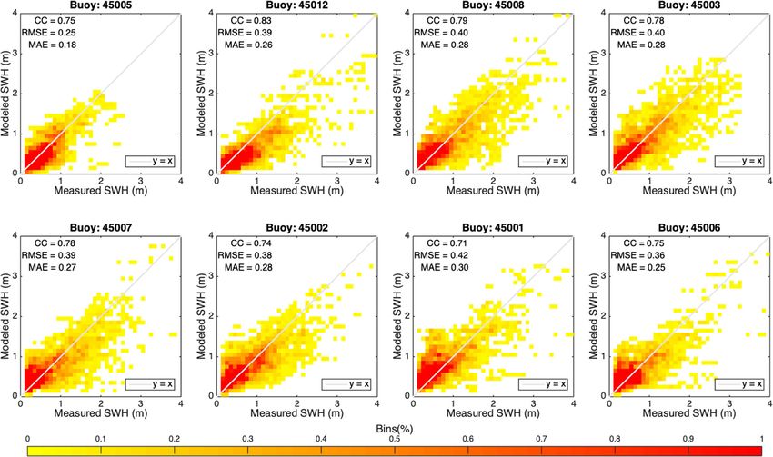
994 Ocean Dynamics (2020) 70:991–1003
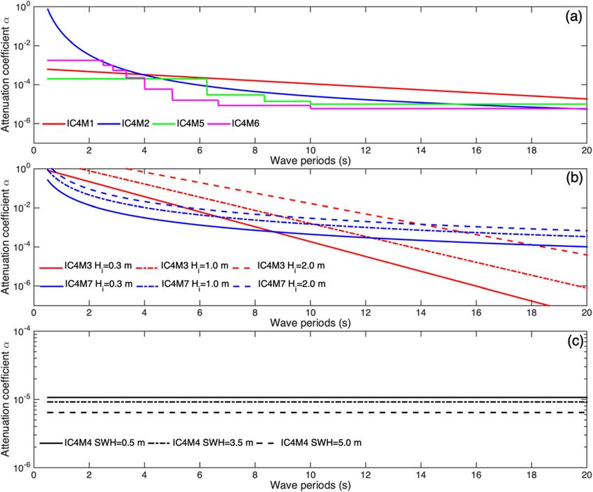
The origins and formulas of IC4M1–M7 are summarized higher frequency the waves, the stronger damping by the
as Table 1. The IC4M1 is exponential as a function of wave ice, which suggests that ice generally acts as a low-pass filter
period, and the coefficients were obtained via an exponential for wave energy (e.g., Squire 2007; Collins and Rogers 2017).
fit to the observations from Wadhams et al. (1988). The The IC4M3 and IC4M7 consider ice thickness as a vital factor
IC4M2 is a 4th degree polynomial fit between α and wave impacting the α, demonstrating that thicker ice has stronger
period based on the measured wave attenuation in the damping ability on waves (Fig. 2b), while IC4M4 reveals
Antarctic by Meylan et al. (2014). Kohout and Meylan stronger waves lose less energy when they pass through ice
(2008) developed a scattering model to calculate wave atten- covered region (Fig. 2c). As Fig. 2 reveals, magnitudes of α
uation, and based on their results, Horvat and Tziperman estimated by different parameterization schemes could differ
(2015) utilized a quadratic equation to fit α, wave period, by several orders, mainly due to the different ice and wave
and ice thickness, i.e., the IC4M3. Kohout et al. (2014) ana- conditions based on which IC4M1–M7 were obtained.
lyzed the same measurements by Meylan et al. (2014) and
found that α is a piecewise function of significant wave height 2.3 Model configuration and numerical experiments
and is independent of wave frequency, i.e., IC4M4. The
IC4M5 is a step function in frequency space with four steps Simulations of lake circulation, waves, and ice were carried
(Doble et al. 2015), and the IC4M6 is identical to IC4M5 but out over the same model domain with the Great Lakes-
with several differences (Rogers et al. 2016), for example, FVCOM (Great Lakes Finite Volume Coastal Ocean Model,
IC4M6 allows up to 10 steps. For the IC4M7, it is a formula developed by Bai et al. 2013), and as Fig. 1a shows, the com-
that depends on wave frequency and ice thickness developed putational mesh covered the entire Great Lakes. Only water
by Doble et al. (2015) using the data collected in the Weddell exchange between Lakes Michigan and Huron was allowed,
Sea. Further details are found in Collins and Rogers (2017) while other lakes were kept separated due to narrow passages
and the WAVEWATCH III® Development Group (2016). between them. The averaged horizontal resolution of this un-
Figure 2 shows the relationships between attenuation coef- structured triangular grid was ~ 3.5 km, and in the vertical
ficient α and wave periods produced by IC4M1–M7. The direction, a 21-layer terrain-following coordinate with higher
Table 1 Summary of the origins and formulas in IC4, where α is attenuation coefficient, T denotes wave period, Hi is ice thickness, SWH is significant
wave height, and f is wave frequency
Method Reference Formula
IC4M1 Wadhams et al. (1988) α = e(−0.18 ∗ T − 0.73)
−3 −2
IC4M2 Meylan et al. (2014) α ¼ 2:12*10
T2
þ 4:59*10
T4
IC4M3 Kohout and Meylan (2008)
α ¼ eð−0:3203þ2:058H i −0:9375T −0:4269H i þ0:1566H i T þ0:0006T 2 Þ
2
Horvat and Tziperman (2015)
8
< 2*5:35*10−6 ðSWH≤ 3Þ
IC4M4 Kohout et al. (2014) α ¼ 2*16:05*10−6
: ðSWH > 3Þ
SWH
8
>
> 2*5:0*10−6 ð f < 0:1Þ
<
2*7:0*10−6 ð0:1 ≤ f < 0:12Þ
α¼ −5
IC4M5 Doble et al. (2015) >
> 2*1:5*10 ð0:12 ≤ f < 0:16Þ
:
2*1:0*10−4 ð f ≥ 0:16Þ
8
>
> 2*2:94*10−6 ð f < 0:1Þ
>
> −6
>
> 2*4:27*10 ð0:1≤ f < 0:15Þ
>
> −6
>
> 2*7:95*10 ð 0:15≤ f < 0:20Þ
<
IC4M6 Rogers et al. (2016) 2*2:95*10−5 ð0:20≤ f < 0:25Þ
α¼
(IC4M6H) >
> 2*1:12*10−4 ð0:25≤ f < 0:30Þ
>
>
>
> 2*2:74*10−4 ð0:30≤ f < 0:35Þ
>
> 2*4:95*10−4 ð0:35≤ f < 0:40Þ
>
>
:
2*8:94*10−4 ð f ≥ 0:40Þ
IC4M7 Doble et al. (2015) α = 0.2 ∗ T−2.13 ∗ Hi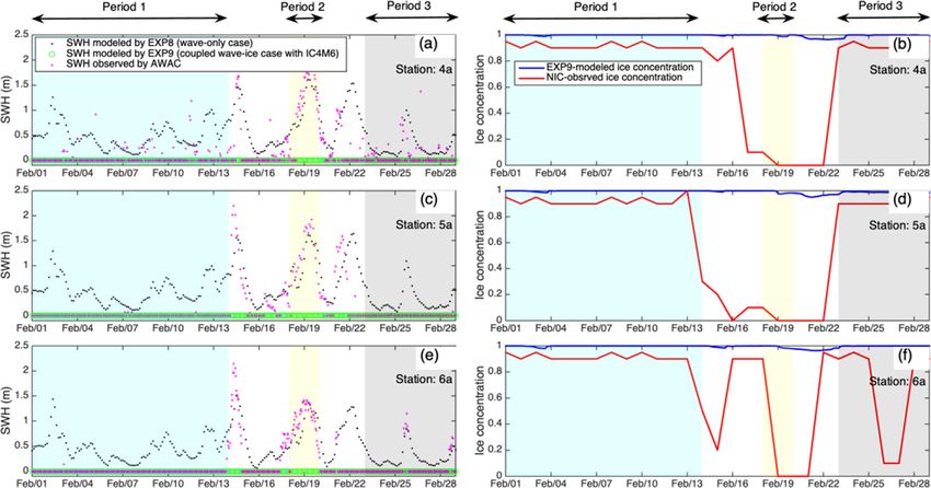
Ocean Dynamics (2020) 70:991–1003                                                                                                        995

Fig. 2 Attenuation coefficient α against the wave periods T (α = f(T))   Hi)) given by IC4M3 and IC4M7 (b). Attenuation coefficient α against
based on IC4M1, IC4M2, IC4M5, and IC4M6 (a). Attenuation                 the wave periods and significant wave height SWH (α = f (T, SWH))
coefficient α against the wave periods and ice thickness Hi (α = f (T,   following IC4M4 (c)

resolution placed near the surface and bottom was adopted.               ratio of 20 was used; meanwhile, a 60-s time step was adopted
The minimum depth was set to 10 m to ensure global stability,            for the ice and wave modules.
i.e., h + ζ > 0 (h is the undisturbed water depth and ζ is the free          A set of numerical experiments designed as Table 2 were
surface elevation, Wang 1996). In this study, the leapfrog               conducted to explore the ice-induced wave attenuation in the
(centered differencing) scheme for time discretization was               Great Lakes. In Table 2, EXP0 was a wave-only modeling
used to replace the Euler forward scheme in the internal mode            case, it was used to examine the performance of the wave
and the Euler forward Runge-Kutta scheme in the external                 module during ice-free season, and it also provided a reference
mode in the integral equations. The reason is that the two-              for those experiments with ice-induced wave attenuation dur-
time-step Euler forward scheme has been proven inertially                ing the ice season. EXP1–EXP7 were coupled wave-ice
unstable, while the leapfrog scheme is inertially neutral stable         modeling cases with both blocking effect and ice-induced
(Wang and Ikeda 1997a, 1997b; Wang et al. 2020, this issue).             wave attenuation, and they used IC4M1–IC4M7 to quantify
Lake circulation, waves, and the ice were driven by the 3-               wave attenuation by ice, respectively. The modeling period of
hourly North American Regional Reanalysis (NARR) prod-                   EXP0–EXP7 were in 2014 because 2014 is a “big chill” year
uct, a long-term set of consistent climate data covering all of          (Fig. 1b) and better understanding of the wave-ice interaction
North and Central America with a 32-km horizontal resolution             under extreme climate conditions is important. EXP8 was
(Mesinger et al. 2006). The wave module resolved wave spec-              identical to EXP0, which was a wave-only modeling case.
tral frequency with 40 frequency bins ranging from 0.04 to               For the EXP9, it was a coupled wave-ice modeling experiment
1 Hz (1 Hz = 1/s) and applied a full cycle direction spectrum            using IC4M6 to calculate ice-induced wave attenuation;
with 36 directional bands. Exponential wave growth and                   meanwhile, blocking effect was also considered. However,
whitecapping functions based on Komen et al. (1984), bottom              the modeling periods of EXP8 and EXP9 were in 2011, when
friction parameterization scheme from Madsen et al. (1989),              there were available wave data observed during the ice season,
and quadruplet wave-wave interactions following                          which therefore could evaluate the performance of the partly
Hasselmann et al. (1973) were utilized. In the circulation mod-          coupled wave-ice model. All numerical runs were initialized
ule, time step for the internal mode was 60 s and a splitting            from a motionless state. To focus on the ice-induced wave
996                                                                                                                 Ocean Dynamics (2020) 70:991–1003

Table 2 Numerical experiments
design of this study               Case      Method quantifying α    Modeling period                    Note

                                   EXP0      N/A                     2014.01.01–2014.12.31              Wave-only modeling
                                   EXP1      IC4M1                   2014.01.01–2014.06.30              Coupled wave-ice modeling with both blocking
                                   EXP2      IC4M2                                                        effect and ice-induced wave attenuation
                                   EXP3      IC4M3
                                   EXP4      IC4M4
                                   EXP5      IC4M5
                                   EXP6      IC4M6
                                   EXP7      IC4M7
                                   EXP8      N/A                     2011.01.01–2011.03.03              Wave-only modeling
                                   EXP9      IC4M6                   2011.01.01–2011.03.03              Coupled wave-ice modeling with both blocking
                                                                                                          effect and ice-induced wave attenuation

attenuation, the feedback from waves to ice, and the dynamics        Figure 3 reveals that the modeled SWH were reasonably con-
related with wave-current interaction were not considered dur-       sistent with the observed ones. To further evaluate the model’s
ing current stage.                                                   performance in simulating lake waves, correlation coef-
                                                                     ficients (CC), root mean square error (RMSE), and
2.4 Observational data                                               mean absolute error (MAE) were applied, and the defi-
                                                                     nitions are given below:
To assess the model’s performance in simulating wave dy-                              ∑Ni¼1 ðxi −xÞðyi −yÞ
namics in Great Lakes, the significant wave height (SWH)             CC ¼ rffiffiffiffiffiffiffiffiffiffiffiffiffiffiffiffiffiffiffiffiffiffiffiffiffiffiffiffi rffiffiffiffiffiffiffiffiffiffiffiffiffiffiffiffiffiffiffiffiffiffiffiffiffiffiffiffi ;          ð3Þ
                                                                            1 N                      2    1 N
in 2014 observed by eight buoys 45001–45003, 45005–                             ∑ ðxi −xÞ                     ∑ ðy −yÞ2
45008, and 45012 (https://www.ndbc.noaa.gov/) were                          N i¼1                        N i¼1 i
                                                                            rffiffiffiffiffiffiffiffiffiffiffiffiffiffiffiffiffiffiffiffiffiffiffiffiffiffiffiffiffi
utilized to validate the modeled SWH, and the buoy                                1 N
locations are illustrated in Fig. 1a. Meanwhile, the buoy-           RMSE ¼           ∑ ðxi −yi Þ2 ;                                             ð4Þ
                                                                                 N i¼1
observed lake surface winds were used to evaluate the quality              1
of the NARR 3-hourly winds over the Great Lakes.                     MAE ¼ ∑Ni¼1 jxi −yi j;                                                      ð5Þ
                                                                           N
   We used the satellite-retrieved ice concentration data, a prod-
uct based on multi-satellite observations (e.g., Radarsat-2,         where N is the total sampling number, xi and yi (i = 1, 2, 3, …,
Envisat, AVHRR, GOES, and MODIS) derived from the                    N-1, N) are the observed and simulated time series of SWH,
National Ice Center (NIC) Great Lakes Ice Analysis Charts            and over bars donate average of the time series. CC, RMSE,
managed and provided by the NOAA Great Lakes                         and MAE correspond to the comparisons at different buoy
Environmental Research Laboratory (https://www.glerl.                stations are shown in the subfigures of Fig. 3, respectively,
noaa.gov/), to appraise the model’s ability in the Great             and overall, CC, RMSE, and MAE for all eight comparisons
Lakes ice dynamics.                                                  were respectively 0.77, 0.38, and 0.26 m, and were compara-
   Wave data measured using the Nortek AWAC (acoustic                ble with former wave simulations for the Great Lakes using
wave and current profiler) at three stations 4a, 5a, and 6a in       third-generation wave models (e.g., Moeini and Etemad-
Lake Erie (locations in Fig. 1c) during February 2011 were           Shahidi 2007; Mao et al. 2016; Niu and Xia 2016). Without
employed to evaluate the performance of the coupled ice-             any calibration, such performance of the wave module was
wave modeling, further details of these wave data are avail-         generally satisfactory and was eligible if for use as the basis
able in Hawley et al. (2018).                                        of coupled wave-ice modeling.
                                                                        Comparisons1 between the NARR winds and the NDBC
                                                                     buoy-observed winds revealed that the averaged differences in
                                                                     wind speed (WSPD) between the NARR winds and winds
3 Modeling the ice-attenuated waves in 2014
                                                                     observed by NDBC buoys 45001–45003, 45005–45008, and
                                                                     45012 (WSPDBuoy–WSPDNARR) in 2014 were − 0.43, 0.53,
3.1 Model performance in wave simulation
                                                                     0.47, 0.87, 0.68, 0.28, 0.84, and 0.85 m/s, respectively,
In the form of scatter diagrams, comparisons between the
                                                                     1
simulated SWH and the ones observed by NDBC buoys at                   Anemometer heights above the ground of NDBC buoys 45001–45003,
eight stations are shown in Fig. 3. Valid wave observations          45005–45008, and 45012 are 5 m, the NARR winds at 10 m were used to
                                                                     force the model, thus the buoy-observed winds were converted to winds at
from the NDBC buoys were only available during ice-free              10 m following a logarithmic relationship for wind speed profile (Allen et al.
time, generally from the mid May to late November, 2014.             1998).
Ocean Dynamics (2020) 70:991–1003 997
Fig. 3 Scatter diagrams of significant wave height: modeled results against the NDBC buoy observations. Scatter diagrams are created by binning the
data into 0.1-m bins, and the gray line indicates function y = x. Model results are from numerical experiment EXP0 (a wave-only case)
suggesting that the model wind forcing (NARR product) gen- the modeled spatial distribution of ice concentration over the
erally underestimated the intensity of lake surface winds Great Lakes in February and March 2014 were examined.
(Fig. 4). Mao et al. (2016) examined the impacts of three Observations showed that Lakes Superior, Huron, and Erie
different wind field sources on wave dynamics in Lake were almost fully covered by ice (Fig. 5 a and b), while there
Michigan; their results demonstrated that accuracy of wind was less ice in Lake Michigan (particularly in the central lake)
forcing is the key factor determining model’s performance with ice concentration ranging from 20 to 50% in most parts.
for waves. Therefore, the relatively weak NARR winds with In Lake Ontario, the whole lake was nearly ice free, which was
low spatiotemporal resolution misjudged the real wind field just as indicated by previous studies (Wang et al. 2018). The
by a certain extent, which was one of the reasons for the errors various ice dynamics in different lakes are mainly caused by
displayed in Fig. 3. In addition to the wind forcing, as many the spatially different climate forcing over each lake; mean-
previous studies revealed, accuracy of the model bathymetry, while, lake ice will respond differently even to the same cli-
resolution and design of the computational grid, choice of mate forcing depending on each lake’s orientation, topogra-
formulations describing the wind input, whitecapping, and phy, and turbidity as revealed by Wang et al. (2018). As dem-
depth-induced wave breaking, as well as consideration of onstrated by Fig. 5, the modeled ice concentration was rea-
wave-current interaction, all could affect the wave model’s sonably consistent with the satellite observations in the form
performance in the Great Lakes (e.g., Mao et al. 2016; Niu of intensity as well as the spatial distribution; furthermore,
and Xia 2016; Mao and Xia 2017). observations revealed increased ice concentration from
February to March, 2014 (Fig. 5 a and b), and this tendency
3.2 Model performance in ice modeling was well reproduced by the model (Fig. 5 c and d), suggesting
reliable model performance in simulating lake ice dynamics.
As illustrated in Sect. 2.2, ice characteristics, including ice
concentration and ice thickness, are the vital parameters deter- 3.3 Ice-induced attenuation on lake waves
mining ice ability to attenuate waves, and therefore, it is nec-
essary to evaluate model’s performance in simulating lake ice. Based on EXP0–EXP7, ice-induced attenuation on lake
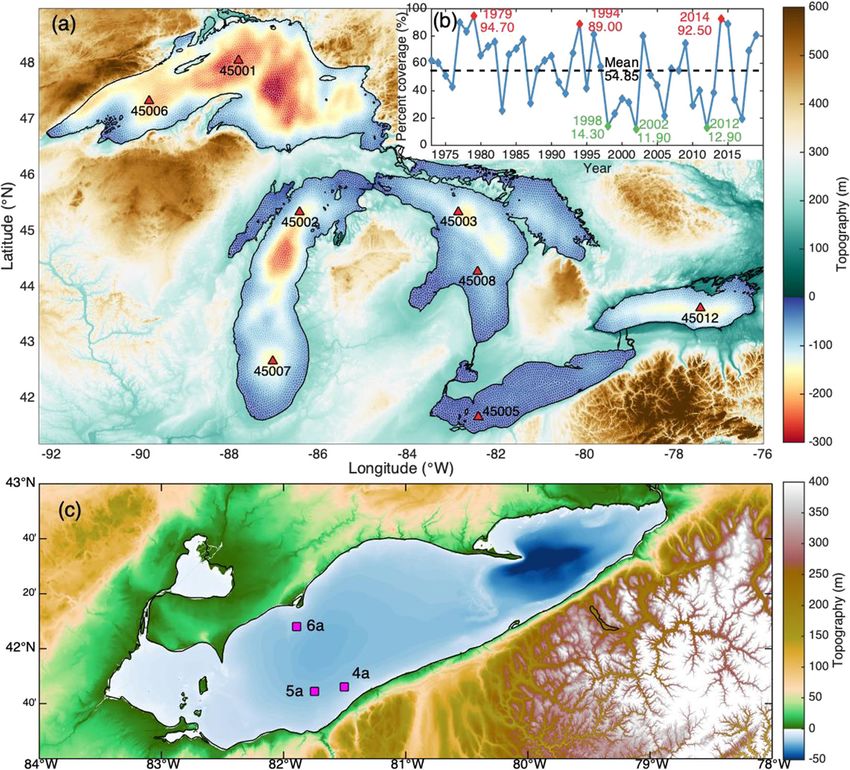
Using the satellite-measured ice concentration from the NIC, waves in February 2014 was evaluated. Figure 6 a shows the998 Ocean Dynamics (2020) 70:991–1003 Fig. 4 Comparisons of the time series of wind speed between the NDBC buoy observations (gray lines) and the NARR product (black lines) during June 1 to December 1, 2014. The mean value of each wind speed time series is marked with red monthly mean SWH in the Great Lakes based on EXP0, and suggested by Table 1 and Fig. 2, the ice-induced wave atten- the monthly averaged differences in SWH between EXP0 and uations quantified by different methods in IC4 were different; EXP1–EXP7 are displayed in Fig. 6b–h, respectively. As meanwhile, the blocking effect of ice on waves remained the Fig. 5 The monthly mean NIC satellite-measured ice concentration over the Great Lakes in February (a) and March (b), 2014, respectively. The simulated spatial distribution of monthly averaged ice concentration over the Great Lakes in February (c) and March (d), 2014, successively
Ocean Dynamics (2020) 70:991–1003                                                                                                    999

Fig. 6 Monthly mean SWH in the Great Lakes based on EXP0 for February 2014 (a). Monthly averaged differences in SWH between EXP0 and EXP1
(b), EXP2 (c), EXP3 (d), EXP4 (e), EXP5 (f), EXP6 (g), and EXP7 (h) in February 2014

same among different numerical runs; therefore, as revealed           there was much less ice (Fig. 5), and the wave attenu-
by Fig. 6b–h, the attenuation of waves by ice simulated by            ation was estimated at approximately 0.2 m (Fig. 6b–h),
EXP1–EXP7 differed from each other.                                   which only counteracted minor parts of the SWH
   Although EXP1–EXP7 simulated different values of                   modeled by EXP0; therefore, significant wave motions
wave attenuation, their spatial patterns were quite simi-             still existed. The weakest wave attenuation was found in
lar to each other. All reasonably revealed that wave                  Lake Ontario, not surprisingly due to the mild lake ice
attenuation by ice was positively correlated with ice                 there (Fig. 5).
concentration. Spatially averaged SWH decreased by                        Note that EXP3 (with IC4M3) and EXP7 (with IC4M7)
0.435, 0.446, 0.467, 0.324, 0.418, 0.424, and 0.450 m                 produced the strongest attenuation (0.467 and 0.450 m); the
over the entire Great Lakes (except Lake Ontario) based               modeled monthly mean ice thickness for February 2014 sug-
on EXP1–EXP7, respectively. In most areas of Lakes                    gested approximately a 0.3-m thick ice over the Great Lakes;
Superior, Huron, and Erie, the reduction of SWH by                    meanwhile, the typical wave period in winter was shorter than
heavy ice (Fig. 6b–h) and the SWH modeled by EXP0                     4 s; thus, under such ice and wave conditions, the attenuation
(Fig. 6a) nearly canceled each other out, suggesting no               coefficients α given by IC4M3 and IC4M7 were generally
wave would develop in these large lakes under heavy-                  larger than other schemes (Fig. 2), which well explains the
ice condition. In the central basin of Lake Michigan,                 stronger wave attenuation estimated by these two methods.
1000                                                                                                        Ocean Dynamics (2020) 70:991–1003

4 Practical application in 2011                                            3 (February 23–March 02, 2011) were selected for further
                                                                           discussions, and these periods are marked with cyan, yellow,
The preceding results strongly indicated that wave-ice inter-              and gray shading in Fig. 7, respectively.
action over the Great Lakes plays a vital role in modifying the               In Period 1, high ice concentration was revealed by both
local hydrodynamic environment, particularly in the wave dy-               the NIC product (approximately 90%) and EXP9 simulation
namics. However, lack of in situ data in 2014 makes it unable              (approximately 100%) at all three AWAC stations (Fig. 7 b, d,
to evaluate the performance of the partly coupled wave-ice                 and f). The AWAC wave observations showed that magni-
model developed in this study. To examine the reliability of               tudes of the SHW at stations 4a, 5a, and 6a were generally
this model, a practical application in the Great Lakes for                 zero, which was accurately modeled by the coupled wave-ice
February 2011 was conducted, during which period wave data                 experiment EXP9, while the wave-only case EXP8 produced
observed by bottom-moored AWAC at three stations (Fig. 1c)                 completely incorrect simulation of the SWH (Fig. 7 a, c, and
are available. Two numerical experiments, EXP8 (wave-only                  e). The detailed statistics (including RMSE and MAE) of
simulation) and EXP9 (coupled wave-ice simulation), were                   SWH comparisons during Period 1 are listed in Table 3, again
performed. For EXP9, both ice-induced wave attenuation                     suggesting good performance of EXP9 in simulating the SWH
and blocking effect of ice on waves were considered, and                   under heavy-ice condition.
the IC4M6 was used to estimate ice-induced wave attenuation                   In Period 2, as indicated by Fig. 7 b, d, and f, remarkable
because this method approximately represented an average of                decreases in ice concentration happened at all three AWAC
IC4M1–M7 (Fig. 6b–h).                                                      stations. During this period, large SWH (even exceeds 2 m)
   Figure 7 a, c, and e show comparisons of the EXP8- and                  were observed at stations 4a, 5a, and 6a, the large SWH pos-
EXP9-modeled SWH with AWAC observations at stations                        sibly indicates that high winds strike Lake Erie, leading to
4a, 5a, and 6a in February 2011, respectively; meanwhile,                  strong mixing in the entire water column, bringing up the
the comparisons between the EXP9-modeled ice concentra-                    warm water from below, and finally melting the ice.
tion and the NIC product for stations 4a, 5a, and 6a are                   Moreover, “ice retreat-wave growth” positive feedback may
displayed in Fig. 7 b, d, and f, respectively; on the basis of             establish during this period: the melt of ice enlarges the area of
the changing trends in the SWH and ice concentration, three                open waters, directly facilitating the growth of waves, while
representative time slots, Period 1 (February 01–February 14,              the strengthened wave dissipation will induce ice breakage,
2011), Period 2 (February 18–February 20, 2011), and Period                accelerating the melting of ice, forming a positive feedback

Fig. 7 Comparisons of the EXP8- and EXP9-modeled SWH with obser-           yellow, and gray shadings mark off Period 1 (February 01–February
vations by AWAC at stations 4a (a), 5a (c), and 6a (e) in February 2011.   14, 2011), Period 2 (February 18–February 20, 2011), and Period 3
The comparisons between the EXP9-modeled ice concentration and the         (February 23–March 02, 2011), correspondingly
NIC product at stations 4a (b), 5a (d), and 6a (f), respectively. Cyan,
Ocean Dynamics (2020) 70:991–1003 1001
Table 3 Statistics of wave
comparisons between EXP8 and Period 1 Period 2 Period 3
EXP9 simulations with the
AWAC observations during RMSE (m) MAE (m) RMSE (m) MAE (m) RMSE (m) MAE (m)
Period 1, 2, and 3 at stations 4a,
5a, and 6a Station 4a EXP8 0.54 0.47 0.47 0.43 0.34 0.27
EXP9 0.05 0.01 1.32 1.11 0.15 0.04
Station 5a EXP8 0.55 0.48 0.40 0.36 0.37 0.30
EXP9 0.01 0.00 1.25 1.14 0.01 0.00
Station 6a EXP8 0.52 0.46 0.35 0.28 0.27 0.23
EXP9 0.06 0.01 1.02 0.95 0.20 0.05
Better statistical results are highlighted with italics
(Zhang et al. 2020). Figure 7 a, c, and e prove that when ice When validated by wave observations from bottom-
concentration is below 10% or even zero, wave dynamics will moored AWAC in Lake Erie during an ice season, the
be generally free of influence by ice, which explains why the model developed in this study satisfactorily reproduced
SWH modeled by the wave-only case EXP8 agreed well with the ice-attenuated waves. Analysis of the AWAC wave
the observations. Note that EXP9 failed to reproduce the data and the satellite-retrieved ice concentration data in-
strong melting process during this period (Fig. 7 b, d, and f) dicated a quick response between waves and ice.
and therefore, remarkably underestimated the SWH (Fig. 7 a, Therefore, accurate ice modeling is necessary for resolv-
d, and e); this may be due to the low spatial resolution of the ing wave-ice interaction because there is a sensitive re-
model, the errors in the NARR forcing, and the neglect of lationship between them.
wave-induced ice breakage. In this study, the ice-induced wave attenuation in the
During Period 3, when high ice concentration (> 80%) cov- Great Lakes was evaluated, and the significance of
ered all three AWAC stations, the results were much similar to wave-ice interaction in the lake hydrodynamics was
that during Period 1, and the statistics summarized in Table 3 demonstrated. The partly coupled wave-ice interaction
again suggest reasonable simulation of SWH by EXP9. Around model provided a foundation for developing a fully
February 14, 19, and 26, 2011, there were three significant coupled wave-ice-lake model for the Great Lakes.
decreases in ice concentration at station 6a, and each decrease However, the feedbacks from waves to ice was not con-
lasted for about 3 days (Fig. 7f); as Fig. 7e reveals, the waves sidered in the present investigation. Therefore, our mod-
responded quite quickly to these ice-decreased events, suggest- el could not produce the “ice retreat-wave growth” pro-
ing a sensitive relationship between waves and ice. cess, which may be one of the main reasons for the
modeling errors in Period 2 of Fig. 7. In the next stage,
it would be interesting to implement effects of waves on
ice into the model, e.g., wave-induced ice breakage. In
5 Summary and conclusions addition, due to the high difficulty, technical require-
ments, and expenses of field observation in ice season,
To better understand how waves and ice interact with each understanding of wave-ice interaction in the Great Lakes
other in the Great Lakes, we developed a partly coupled (also other cold regions) is limited by the scarcity of
wave-ice interaction model with the ability to resolve the ice- simultaneous wave and ice observations, and further
induced wave attenuation within the FVCOM framework. The field observations regarding wave-ice interaction under
WAVEWATCH III® IC4 was utilized to quantify the wave various ice and wave conditions are necessary in the
energy loss when propagating under ice. Meanwhile, the future.
blocking effect of ice on wind energy input and wave energy
decay via whitecapping and breaking were also implemented. Acknowledgments We gratefully thank the two anonymous reviewers
for providing constructive and insightful comments, which have contrib-
The model was then applied to the Great Lakes, and a set of
uted to the substantial improvements of the manuscript. Peng Bai ac-
numerical experiments were conducted to assess the reduction knowledges a grant from the National Research Council Research
of wave height in the presence of ice. Numerical results dem- Associateship Programs. This research was partially funded by NSF
onstrated that the ice-induced wave attenuation and the ice Grant OCE 0927643 to Dmitry Beletsky. We would like to thank
Songzhi Liu for his assistance in processing the NIC ice concentration
concentration were positively correlated. In February 2014,
data. This is GLERL Contribution No. 1946. Funding was awarded to the
there were almost no wind wave motions in Lakes Superior, Cooperative Institute for Great Lakes Research (CIGLR) through the
Huron, and Erie because the heavy ice there could remarkably NOAA Cooperative Agreement with the University of Michigan
inhibit the growth and development of wind waves. (NA17OAR4320152). This CIGLR contribution number is 1160.1002 Ocean Dynamics (2020) 70:991–1003
References Fujisaki-Manome A, Wang J (2016) Simulating hydrodynamics and ice
cover in Lake Erie using an unstructured grid model. Proceedings of
23th IAHR International Symposium on Ice (2016)
Allen RG, Pereira LS, Raes D, Smith M (1998) Crop evapotranspiration-
Gao G, Chen C, Qi J, Beardsley RC (2011) An unstructured-grid, finite-
guidelines for computing crop water requirements-FAO irrigation
volume sea ice model: development, validation, and application.
and drainage paper 56. Fao, Rome 300(9):D05109
Journal of Geophysical Research: Oceans 116(C8)
Anderson E, Fujisaki-Manome A, Kessler J, Lang G, Chu P, Kelley J,
Hasselmann K, Barnett TP, Bouws E, Carlson H, Cartwright DE, Enke K,
Wang J (2018) Ice forecasting in the next-generation Great Lakes
Meerburg A (1973) Measurements of wind-wave growth and swell
Operational Forecast System (GLOFS). J Mar Sci Eng 6(4):123
decay during the Joint North Sea Wave Project (JONSWAP).
Ardhuin F, Roland A, Dumas F, Bennis A-C, Sentchev A, Forget P, Wolf Ergänzungsheft:8–12
J, Girard F, Osuna P, Benoit M (2012) Numerical Wave Modeling Hawley N, Beletsky D, Wang J (2018) Ice thickness measurements in
in Conditions with Strong Currents: Dissipation, Refraction, and Lake Erie during the winter of 2010–2011. J Great Lakes Res 44(3):
Relative Wind. J Phys Oceanogr 42(12):2101–2120 388–397
Bai X, Wang J, Sellinger C, Clites A, Assel R (2012) Interannual vari- Horvat C, Tziperman E (2015) A prognostic model of the sea-ice floe size
ability of Great Lakes ice cover and its relationship to NAO and and thickness distribution. Cryosphere 9(6):2119–2134
ENSO. J Geophys Res: Oceans 117(C3) Hubertz JM, Driver DB, Reinhard RD (1991) Wind waves on the Great
Bai X, Wang J, Schwab DJ, Yang Y, Luo L, Leshkevich GA, Liu S Lakes: a 32 year hindcast. J Coast Res:945–967
(2013) Modeling 1993–2008 climatology of seasonal general circu- Hunke EC, Lipscomb WH, Turner AK, Jeffery N, Elliott S (2010) CICE:
lation and thermal structure in the Great Lakes using FVCOM. the Los Alamos Sea ice model documentation and software User’s
Ocean Model 65:40–63 manual version 4.1 LA-CC-06-012. T-3 Fluid Dynamics Group,
Bai X, Wang J, Austin J, Schwab DJ, Assel R, Clites A, Wohlleben T Los Alamos National Laboratory, 675
(2015) A record-breaking low ice cover over the Great Lakes during Kohout AL, Meylan MH, Sakai S, Hanai K, Leman P, Brossard D (2007)
winter 2011/2012: combined effects of a strong positive NAO and Linear water wave propagation through multiple floating elastic
La Niña. Clim Dyn 44(5–6):1187–1213 plates of variable properties. J Fluids Struct 23(4):649–663
Barber DG, Galley R, Asplin MG, De Abreu R, Warner KA, Pućko M, Kohout AL, Meylan MH (2008) An elastic plate model for wave attenu-
Julien S (2009) Perennial pack ice in the southern Beaufort Sea was ation and ice floe breaking in the marginal ice zone. J Geophys Res:
not as it appeared in the summer of 2009. Geophys Res Lett 36(24) Oceans 113(C9)
Beletsky D, Saylor JH, Schwab DJ (1999) Mean circulation in the Great Kohout AL, Williams MJM, Dean SM, Meylan MH (2014) Storm-
Lakes. J Great Lakes Res 25(1):78–93 induced sea-ice breakup and the implications for ice extent. Nature
Bennetts LG, Squire VA (2009) Wave scattering by multiple rows of 509(7502):604–607
circular ice floes. J Fluid Mech 639:213–238 Kohout AL, Williams MJM, Toyota T, Lieser J, Hutchings J (2016) In
Bennetts LG, Squire VA (2011) On the calculation of an attenuation situ observations of wave-induced sea ice breakup. Deep-Sea Res II
coefficient for transects of ice-covered ocean. Proceedings of the Top Stud Oceanogr 131:22–27
Royal Society A: Mathematical, Physical and Engineering Komen GJ, Hasselmann K, Hasselmann K (1984) On the existence of a
Sciences 468(2137):136–162 fully developed wind-sea spectrum. J Phys Oceanogr 14(8):1271–
Booij NRRC, Ris RC, Holthuijsen LH (1999) A third-generation wave 1285
model for coastal regions: 1. Model description and validation. J Lou J, Schwab DJ, Beletsky D, Hawley N (2000) A model of sediment
Geophys Res Oceans 104(C4):7649–7666 resuspension and transport dynamics in southern Lake Michigan. J
Brissette FP, Tsanis IK, Wu J (1993) Wave directional spectra and wave- Geophys Res: Oceans 105(C3):6591–6610
current interaction in Lake St. Clair. J Great Lakes Res 19(3):553– Madsen, O. S., Poon, Y. K., Graber, H. C. 1989. Spectral wave attenua-
568 tion by bottom friction: theory. In Coastal Engineering 1988 (pp.
492-504)
Brown RW, Taylor WW, Assel RA (1993) Factors affecting the recruit-
Mao M, Xia M (2017) Dynamics of wave–current–surge interactions in
ment of lake whitefish in two areas of northern Lake Michigan. J
Lake Michigan: a model comparison. Ocean Model 110:1–20
Great Lakes Res 19(2):418–428
Mao M, Van Der Westhuysen AJ, Xia M, Schwab DJ, Chawla A (2016)
Campbell AJ, Bechle AJ, Wu CH (2014) Observations of surface waves Modeling wind waves from deep to shallow waters in Lake
interacting with ice using stereo imaging. J Geophys Res Oceans Michigan using unstructured SWAN. J Geophys Res: Oceans
119(6):3266–3284 121(6):3836–3865
Chen C, Liu H, Beardsley RC (2003) An unstructured grid, finite-vol- Mesinger F, DiMego G, Kalnay E, Mitchell K, Shafran PC, Ebisuzaki W,
ume, three-dimensional, primitive equations ocean model: applica- Ek MB (2006) North American regional reanalysis. Bull Am
tion to coastal ocean and estuaries. J Atmos Ocean Technol 20(1): Meteorol Soc 87(3):343–360
159–186 Meylan MH, Bennetts LG, Kohout AL (2014) In situ measurements and
Collins CO, Rogers WE (2017) A source term for wave attenuation by sea analysis of ocean waves in the Antarctic marginal ice zone. Geophys
ice in WAVEWATCH III®: IC4. NRL report NRL/MR/7320–17- Res Lett 41(14):5046–5051
9726, 25 pp. [available from www7320. Nrlssc. Navy. Mil/pubs. Moeini MH, Etemad-Shahidi A (2007) Application of two numerical
Php] models for wave hindcasting in Lake Erie. Appl Ocean Res 29(3):
De Santi F, De Carolis G, Olla P, Doble M, Cheng S, Shen HH, Thomson 137–145
J (2018) On the ocean wave attenuation rate in grease-pancake ice, a Niimi AJ (1982) Economic and environmental issues of the proposed
comparison of viscous layer propagation models with field data. J extension of the winter navigation season and improvements on
Geophys Res: Oceans 123(8):5933–5948 the Great Lakes-St. Lawrence Seaway system. J Great Lakes Res
Doble MJ, De Carolis G, Meylan MH, Bidlot JR, Wadhams P (2015) 8(3):532–549
Relating wave attenuation to pancake ice thickness, using field mea- Niu Q, Xia M (2016) Wave climatology of Lake Erie based on an
surements and model results. Geophys Res Lett 42(11):4473–4481 unstructured-grid wave model. Ocean Dyn 66(10):1271–1284
Dumont D, Kohout A, Bertino L (2011) A wave-based model for the Niu Q, Xia M (2017) The role of wave-current interaction in Lake Erie’s
marginal ice zone including a floe breaking parameterization. J seasonal and episodic dynamics. J Geophys Res Oceans 122(9):
Geophys Res: Oceans 116(C4) 7291–7311Ocean Dynamics (2020) 70:991–1003 1003
Pleskachevsky A, Eppel DP, Kapitza H (2009) Interaction of waves, for polynomials on the unit circle. Mon Weather Rev 124(6):1301–
currents and tides, and wave-energy impact on the beach area of 1310
Sylt Island. Ocean Dyn 59(3):451–461 Wang J, Ikeda M (1997a) Inertial stability and phase error of time inte-
Qi J, Chen C, Beardsley RC, Perrie W, Cowles GW, Lai Z (2009) An gration schemes in ocean general circulation models. Mon Weather
unstructured-grid finite-volume surface wave model (FVCOM- Rev 125(9):2316–2327
SWAVE): Implementation, validations and applications. Ocean Wang J, Ikeda M (1997b) Diagnosing ocean unstable baroclinic waves
Model 28(1-3):153–166 and meanders using the quasigeostrophic equations and Q-vector
Ris RC, Holthuijsen LH, Booij N (1999) A third-generation wave model method. J Phys Oceanogr 27(6):1158–1172
for coastal regions: 2. Verification. J Geophys Res Oceans 104(C4): Wang R, Shen HH (2011) A continuum model for the linear wave prop-
7667–7681 agation in ice-covered oceans: an approximate solution. Ocean
Rogers WE, Thomson J, Shen HH, Doble MJ, Wadhams P, Cheng S Model 38(3–4):244–250
(2016) Dissipation of wind waves by pancake and frazil ice in the Wang J, Bai X, Hu H, Clites A, Colton M, Lofgren B (2012) Temporal
autumn Beaufort Sea. J Geophys Res: Oceans 121(11):7991–8007 and spatial variability of Great Lakes ice cover, 1973–2010. J Clim
Schwab DJ, Beletsky D (2003) Relative effects of wind stress curl, to- 25(4):1318–1329
pography, and stratification on large-scale circulation in Lake
Wang J, Kessler J, Bai X, Clites A, Lofgren B, Assuncao A, Leshkevich
Michigan. J Geophys Res: Oceans 108(C2)
G (2018) Decadal variability of Great Lakes ice cover in response to
Sellinger CE, Stow CA, Lamon EC, Qian SS (2007) Recent water level
AMO and PDO, 1963–2017. J Clim 31(18):7249–7268
declines in the Lake Michigan− Huron System. Environ Sci Technol
Wang J, Manome A, Kessler J, Zhang S, Chu P, Peng S, Zhu X,
42(2):367–373
Anderson E (2020) Inertial instability and phase error in third- and
Squire VA (2007) Of ocean waves and sea-ice revisited. Cold Reg Sci
fourth-stage predictor-corrector time integration schemes in ocean
Technol 49(2):110–133
circulation models: application to Great Lakes modeling. Ocean
The WAVEWATCH III® Development Group (WW3DG) (2016) User
Dynamics (submitted)
manual and system documentation of WAVEWATCH III® version
5.16. Tech. Note 329, NOAA/NWS/NCEP/MMAB, College Park, Williams TD, Bennetts LG, Squire VA, Dumont D, Bertino L (2013)
MD, USA, 326 pp. + Appendices Wave–ice interactions in the marginal ice zone. Part 1: theoretical
Vanderploeg HA, Bolsenga SJ, Fahnenstiel GL, Liebig JR, Gardner WS foundations. Ocean Model 71:81–91
(1992) Plankton ecology in an ice-covered bay of Lake Michigan: Wright DM, Posselt DJ, Steiner AL (2013) Sensitivity of lake-effect
utilization of a winter phytoplankton bloom by reproducing cope- snowfall to lake ice cover and temperature in the Great Lakes region.
pods. Hydrobiologia 243(1):175–183 Mon Weather Rev 141(2):670–689
Vaughan GL, Squire VA (2011) Wave induced fracture probabilities for Xue P, Pal JS, Ye X, Lenters JD, Huang C, Chu PY (2017) Improving the
arctic sea-ice. Cold Reg Sci Technol 67(1-2):31–36 simulation of large lakes in regional climate modeling: two-way
Vavrus S, Notaro M, Zarrin A (2013) The role of ice cover in heavy lake- lake–atmosphere coupling with a 3D hydrodynamic model of the
effect snowstorms over the Great Lakes Basin as simulated by Great Lakes. J Clim 30(5):1605–1627
RegCM4. Mon Weather Rev 141(1):148–165 Zhang Y, Chen C, Beardsley RC, Gao G, Qi J, Lin H (2016) Seasonal and
Vincent CE (1979) The Interaction of Wind-Generated Sea Waves with interannual variability of the Arctic sea ice: a comparison between
Tidal Currents. J Phys Oceanogr 9(4):748–755 AO-FVCOM and observations. J Geophys Res: Oceans 121(11):
Wadhams P, Squire VA, Goodman DJ, Cowan AM, Moore SC (1988) 8320–8350
The attenuation rates of ocean waves in the marginal ice zone. J Zhang Y, Chen C, Beardsley RC, Perrie W, Gao G, Zhang Y, Lin H
Geophys Res: Oceans 93(C6):6799–6818 (2020) Applications of an unstructured grid surface wave model
Wang J (1996) Global linear stability of the two-dimensional shallow- (FVCOM-SWAVE) to the Arctic Ocean: the interaction between
water equations: an application of the distributive theorem of roots ocean waves and sea ice. Ocean Model 145:101532You can also read