The First Wave of the COVID-19 Pandemic and Its Impact on Socioeconomic Inequality in Psychological Distress in the UK - IZA DP No. 14057 JANUARY 2021

DISCUSSION PAPER SERIES

IZA DP No. 14057

The First Wave of the COVID-19 Pandemic
and Its Impact on Socioeconomic
Inequality in Psychological Distress
in the UK
Apostolos Davillas
Andrew M. Jones

JANUARY 2021

DISCUSSION PAPER SERIES

IZA DP No. 14057

The First Wave of the COVID-19 Pandemic
and Its Impact on Socioeconomic
Inequality in Psychological Distress
in the UK
Apostolos Davillas
University of East Anglia and IZA
Andrew M. Jones
University of York and Monash University

JANUARY 2021

Any opinions expressed in this paper are those of the author(s) and not those of IZA. Research published in this series may
include views on policy, but IZA takes no institutional policy positions. The IZA research network is committed to the IZA
Guiding Principles of Research Integrity.
The IZA Institute of Labor Economics is an independent economic research institute that conducts research in labor economics
and offers evidence-based policy advice on labor market issues. Supported by the Deutsche Post Foundation, IZA runs the
world’s largest network of economists, whose research aims to provide answers to the global labor market challenges of our
time. Our key objective is to build bridges between academic research, policymakers and society.
IZA Discussion Papers often represent preliminary work and are circulated to encourage discussion. Citation of such a paper
should account for its provisional character. A revised version may be available directly from the author.

 ISSN: 2365-9793

 IZA – Institute of Labor Economics
Schaumburg-Lippe-Straße 5–9 Phone: +49-228-3894-0
53113 Bonn, Germany Email: publications@iza.org www.iza.org

IZA DP No. 14057 JANUARY 2021

 ABSTRACT
 The First Wave of the COVID-19 Pandemic
 and Its Impact on Socioeconomic
 Inequality in Psychological Distress
 in the UK*
 We use data from the UK Household Longitudinal Study (UKHLS) to compare measures
 of socioeconomic inequality in psychological distress, measured by the General Health
 Questionnaire (GHQ), before (Waves 9 and the Interim 2019 Wave) and during the first
 wave of the COVID-19 pandemic (April to July 2020). Based on a caseness measure, the
 prevalence of psychological distress increased from 18.5% to 27.7% between the 2019
 Wave and April 2020 with some reversion to earlier levels in subsequent months. Also,
 there was a systematic increase in total inequality in the Likert GHQ-12 score. However,
 measures of relative socioeconomic inequality have not increased. A Shapley-Shorrocks
 decomposition analysis shows that during the peak of the first wave of the pandemic (April
 2020) other socioeconomic factors declined in their share of socioeconomic inequality,
 while age and gender account for a larger share. The most notable increase is evident
 for younger women. The contribution of working in an industry related to the COVID-
 19 response played a small role at Wave 9 and the Interim 2019 Wave, but more than
 tripled its share in April 2020. As the first wave of COVID-19 progressed, the contribution
 of demographics declined from their peak level in April and chronic health conditions,
 housing conditions, and neighbourhood characteristics increased their contributions to
 socioeconomic inequality.

 JEL Classification: C1, D63, I12, I14
 Keywords: COVID-19, health equity, socioeconomic inequality, GHQ,
 mental health, psychological distress

 Corresponding author:
 Andrew M. Jones
 Department of Economics and Related Studies
 University of York
 York, YO10 5DD
 United Kingdom
 E-mail: andrew.jones@york.ac.uk

 * Understanding Society is an initiative funded by the Economic and Social Research Council and various Government
 Departments, with scientific leadership by the Institute for Social and Economic Research, University of Essex, and
 survey delivery by NatCen Social Research and Kantar Public. The research data are distributed by the UK Data Service.
 Andrew Jones acknowledges funding from the Leverhulme Trust Major Research Fellowship (MRF-2016-004). The
 funders, data creators and UK Data Service have no responsibility for the contents of this paper. We are grateful to
 Stephen Jenkins, Nicolas Pistolesi, Carol Propper and two anonymous reviewers for their comments on an earlier
 version.

1 Introduction
Has the experience of the COVID-19 pandemic in the UK had a greater impact on
psychological distress among those in more disadvantaged pre-existing circumstances
and hence widened socioeconomic inequalities? The UK Household Longitudinal Study
(UKHLS), Understanding Society, launched a COVID-19 survey to examine the impact
of the coronavirus pandemic on UKHLS participants. The release of these data provides
an opportunity to address this question. The survey has been sent to adult UKHLS
participants once a month with the first release collected in April 2020 (Institute for
Social and Economic Research, 2020). We use data from UKHLS Wave 9 and the
Interim 2019 Wave, along with the April 2020 and three subsequent releases of the
COVID-19 web survey to compare measures of socioeconomic inequality in mental
health. Mental health is measured by the General Health Questionnaire (GHQ), which
captures twelve indicators of psychological distress. This allows us to compare the
distribution of GHQ before and during the first wave of the pandemic in the UK.

COVID-19 originated in the city of Wuhan, China, in December 2019 and spread rapidly
to become a global pandemic. Wednesday 29th January saw the first two patients test
positive for COVID-19 in the UK. On 11th March the UK Government announced its first
package of financial support for those affected and on the same day the World Health
Organisation (WHO) declared a global pandemic. The following week saw the
announcement of a much larger financial package in the UK. The closure of pubs,
restaurants, gyms and other social venues was announced on Friday 20th March and
then on 23rd March a national lockdown was announced. This lockdown included the
shielding on 1.5 million vulnerable people and the public as a whole were instructed to
begin socially isolating and expected to stay at home. The exceptions to this were for
essential workers and for non-essential workers who were not able to work from home,
shopping for essentials such as food and medical supplies, medical reasons, providing
help to the vulnerable, and taking exercise once a day. It was not until 13th May that the
first easing of lockdown was announced; two subsequent easings of lockdown were made
on the 1st and 15th of June with a further easing on the 4th of July1.

By April 2020, when our new data were first collected, the UK appeared to be at the
peak of the first phase of the pandemic. The direct impact of COVID-19 on health and
wellbeing had caused 20,283 COVID-19 registered deaths in England and Wales up to
17th April. The pandemic highlighted existing socioeconomic inequalities in health and
appears to have amplified the gradients in health by age, sex, ethnicity, income and
wealth, education and housing. For example, the end of April coincided with the
publication of evidence from the Office for National Statistics (2020a) that revealed a
stark social gradient in the mortality rates associated with COVID-19. Comparisons of

1 COVID-19 policy tracker. The Heath Foundation. https://www.health.org.uk/news-
andcomment/charts-and-infographics/covid-19-policy-tracker.

 1

data up to 17th April 2020 showed substantial socio-geographic variation in death rates
across local authorities in England and Wales2.

The nature of the economic and policy response to COVID-19 has created specific
gradients in both exposure to the disease itself and in exposure to the economic impact
of the lockdown. These new or amplified facets of existing socioeconomic inequalities
include, for example, those working in essential occupations (for example, in health and
social care and other public services), financial and employment hardship, the presence
of children in households and living in multigenerational households or as lone parents.
Moreover, other facets include the influence of housing and neighbourhood environment
on people’s ability to self-isolate.

Beyond the direct impact of COVID-19, the population as a whole has been exposed to
the policy response to the pandemic. Lockdown, social distancing, self-isolation, the
economic impact of shut-down of parts of the economy and the focusing of resources
within the health and social care systems on coping with the pandemic may all have had
an indirect impact on psychological distress and the mental health of the population
(e.g., Haiyang et al., 2020). Given the characteristics of the policy and institutional
responses outlined above, the burden of this psychological distress may have been
unequally distributed within the population according to their pre-existing
circumstances. This is what we seek to explore in this paper.

To measure the impact of the UK response to the pandemic in terms of socioeconomic
inequalities in health we build on methodological approaches that use the notion of
equality of opportunity (e.g., Ramos and Van de Gaer, 2016; Roemer and Trannoy,
2016). The equality of opportunity perspective tends to focus on early life circumstances
as the source of unfair or illegitimate inequalities in the outcome of interest. In this
paper, we broaden that perspective and, to provide additional insights into the impact of
the pandemic on socioeconomic inequity, we include factors that are specific to the policy
debate concerning the adverse consequences of COVID-19 for social inequality. In doing
this we follow the spirit of Fleurbaey and Schokkaert (2009) and regard these factors,
which were pre-existing prior to the onset of the pandemic, as a source of unfair, or
inequitable, variation in health outcomes. To put this approach into practice we use
well-established techniques that have been applied to the measurement of inequality of
opportunity; we follow Davillas and Jones (2020), adapting and broadening their
approach.

We compare the GHQ measure of psychological distress before (at UKHLS Wave 9 and
at the 2019 Wave), at the peak of the initial phase of coronavirus (April 2020), and then
in May, June and July 2020. The results show a substantial and systematic worsening
of the levels of GHQ post-COVID. This applies to nearly all of the individual elements of

2
 Specifically, the most deprived London boroughs had the highest COVID-19 age-standardised
death rates with Newham at 144.3 deaths per 100,000, Brent at 141.5 and Hackney at 127.4
compared to an average of 36.2 per 100,000 in England and Wales as a whole.

 2

GHQ and to overall GHQ scores. For example, the prevalence of psychological distress
based on the GHQ-12 caseness scoring, increased from 18.5% at the 2019 Wave to 27.7%
at the peak in April 2020. In addition, there is a statistically significant increase in total
inequality in the Likert GHQ-12 score between the data collected before and during the
pandemic. However, we find no increase in relative socioeconomic inequality in April
2020 and subsequent months, suggesting that the proportion of total inequality
attributed to observed circumstances has not increased with COVID-19. A Shapley-
Shorrocks decomposition analysis allows us to explore the contribution of specific
circumstances. During the peak of the UK response to the first wave of the pandemic
(April 2020) key socioeconomic factors declined in their share of socioeconomic
inequality and age and gender accounted for a larger share. As the pandemic progressed
towards July 2020, the contribution of demographics declined from their peak levels and
chronic health conditions, housing conditions, household composition and neighbourhood
characteristics increased their contributions to socioeconomic inequality.

2 Methods
2.1 Measuring socioeconomic inequality in psychological distress
We assume that the observed realisations of an individual’s mental health can be
expressed as:
 ℎ = ( , ( , ), ) (1)
where h is the specific mental health outcome of interest. In the language of inequality
of opportunity, C are observed circumstances and E is a vector of efforts of inequality
(which need not be observed)3. In the IOp literature these circumstances have typically
been associated with early life circumstances. A broader interpretation is provided by
Fleurbaey and Schokkaert’s (2009) model of unfair health inequalities in which the C
are defined generally as illegitimate, or unfair, sources of inequality and E as legitimate,
or fair, sources of inequality. As described above, we take a broader view of the sources
of socioeconomic inequalities that are regarded as a concern in the context of COVID-19
and we define the list of observed circumstances accordingly; these circumstances are
predetermined with respect to the COVID-19 pandemic.

3
 Roemer (1998) defines a ‘responsibility cut’ that partitions all factors influencing individual
attainment between a category of effort factors, for which individuals should be held partly
responsible, and a category of circumstance factors, which are judged to be a source of unfair
differences in outcomes. The concept of equality of opportunity draws on two ethical principles:
compensation and reward (e.g., Fleurbaey and Schokkaert, 2012). There are two broad
perspectives on the definition and measurement of inequality of opportunity: the ex ante and the
ex post approaches. The ex ante approach defines equality of opportunity if all individuals face
the same opportunity set, prior to their efforts and outcomes being realised; then, individuals
have equal opportunities if there are no differences in expected outcomes across types who have
different circumstances. The expectation over outcomes within types can be based on a simple
mean (utilitarian reward) or with some degree of inequality aversion within types.

 3

The specification of equation (1) includes unobserved error terms to reflect that observed
realisations of mental health outcomes are random; specifically, captures random
variation in effort that is independent of C, while captures random variation in
outcomes, including any measurement error, that is independent of C and E. Mental
health outcomes are the realisations of a random process and we make no judgement
about whether the unexplained component of these outcomes reflects unobserved
circumstances, unobserved effort, measurement error or pure chance and, hence,
whether the unexplained variation is legitimate or not4. Our focus is on measuring the
component that can be attributed to the observed circumstance factors C.

Then, assuming additive separability and linearity of (. ) and (. ), a linear reduced
form can be derived (see e.g., Carrieri et al. (2020) for a derivation):
 ℎ = + (2)

where the coefficients reflect the total contribution of circumstances and include both
the direct contribution of circumstances and their indirect contribution through their
influence on efforts5. Linearity may be regarded as a restrictive assumption but it is
needed to derive the linear reduced form and hence to provide us with a tractable
decomposition analysis and empirical results that are open to an intuitive
interpretation. We follow Davillas and Jones (2020) and adopt an approach based on ex
ante compensation and utilitarian reward that focuses on inequality in the distribution
of mean outcomes conditional on observed circumstances6. In practice, the mean-based
direct parametric approach is based on using predictions of (ℎ | ) from the reduced
form regression (2) as the counterfactual outcome:
 ℎ̃ = ̂ (3)
These predicted outcomes are the same for all individuals with identical circumstances
and all of the variation in ℎ̃ is attributable to differences in their observed circumstances
(Ferreira and Gignoux, 2011; Wendelspeiss Chávez Juárez and Soloaga, 2014)7. The

4 One of the sources of potential measurement error in GHQ outcomes may be the mixed
interview modes (web versus face-to-face surveys) used in the baseline and subsequent COVID-
19 waves regarding the GHQ questionnaire. However our conclusions are unlikely to be
contaminated by any potential measurement error due to interview mode (see footnote 13 and
Appendix C).
5 A feature of this approach is that the distribution of effort within each type constitutes a

circumstance in itself. The model therefore assumes that effort is a function of circumstances,
with circumstances being pre-determined. The reduced form (2) captures both direct and indirect
contributions of circumstances.
6
 Here we differ from the approach taken to health equity in Fleurbaey and Schokkaert (2009)
who work within an ex post framework, based on a model like equation (1) that conditions on
both C and E, from which they derive two different standardised measures of the outcome: the
fairness gap and the direct unfairness measures. Their approach requires E to be defined and
observed.
7
 Given that some of our mental health outcomes are binary variables, a probit model is used to
estimate the conditional probability function, given our set of circumstances, and the relevant
counterfactual predictions are obtained (analogously to, equations 2 and 3).

 4

level of observed socioeconomic inequality can be estimated using a suitable inequality
measure, I(.), applied to the vector of counterfactual outcomes ℎ̃:
 = I(ℎ̃) (4)
The fraction of the overall inequality in mental health functioning that is attributed to
observed socioeconomic inequality can be expressed as a percentage share of total
inequality:
 ̃)
 I(ℎ
 = (ℎ) . 100 (5)

We present results for three sets of mental health outcomes, all derived from the GHQ.
These measures are compared between UKHLS Wave 9 and the 2019 Wave, the COVID-
19 data for April 2020 and subsequent waves of the web survey.

The GHQ is a widely used instrument to measure non-psychotic psychological distress
and we use it to define three sets of outcomes. The first are binary indicators for each of
the twelve questions that comprise the GHQ questionnaire (see Appendix A for full
details). These collapse the responses to the twelve dimensions of GHQ into, so-called,
caseness binary indicators. To measure I(ℎ̃), we apply the dissimilarity index to each of
these8. These indicators allow us to explore inequalities in each of the GHQ dimensions
and, thus, identify which of the dimensions of physiological distress were most affected
by the response to the pandemic.

The second outcome is the level of GHQ-12 measured on a continuous Likert scale that
sums the 12 components of the GHQ. Previous studies have argued that the mean
logarithmic deviation (MLD) or the variance are relevant inequality indexes to be used
for continuous outcomes, depending on the nature of the outcome variable (e.g., Davillas
and Jones, 2020; Carrieri et al., 2020; Ferreira and Gignoux, 2011, 2013; Wendelspeiss
Chávez Juárez and Soloaga, 2014). As the Likert GHQ-12 score is not a ratio-scaled
variable, the variance of ℎ̃ is used as our main inequality measure I(ℎ̃) (Carrieri et al.,
2020; Wendelspeiss Chávez Juárez and Soloaga, 2014)9. Then the IOp share, , is
measured by the share of the total variance in our continuous mental health measure
that is attributed to observed circumstances. For comparison, we also provide results
using the MLD inequality measure.

The third outcome is an indicator based on dichotomising the overall GHQ-12 index,
which is constructed by the caseness scoring method, using appropriate thresholds. To
measure socioeconomic inequality the dissimilarity index is applied to this indicator.

As discussed above, for the level of GHQ-12 Likert score, which is a continuous non-ratio
scale measure, we use the variance as our main inequality measure with:

8 Dissimilarity indexes have been used by the World Bank to compute the Human Opportunity
Index (e.g., Paes de Barros et al., 2009).
9 The variance has been proposed as an inequality measure in a number of recent contributions

to the IOp literature (see, e.g., Carrieri & Jones, 2018; Fleurbaey & Schokkaert, 2009, 2012;
Jusot et al., 2013).

 5

1 2
 I(. ) = ∑ =1(ℎ̃ − ℎ̅) (6)

where the predicted conditional means ℎ̃ are estimated using linear regression models.
For our binary outcomes, we use the dissimilarity index (Paes de Barros et al., 2007;
Wendelspeiss Chávez Juárez and Soloaga, 2014):
 2
 I(. ) = ℎ̅ ∑ =1|ℎ̃ − ℎ̅| (7)

where the predicted sample proportions ℎ̃ are estimated using probit models.

2.2 Decomposing the socioeconomic inequality in health
We use a Shapley-Shorrocks decomposition to measure the contribution of the measured
circumstance variables (C) to overall socioeconomic inequality (Davillas and Jones, 2020;
Deutsch, et al., 2018; Shorrocks, 2013; Wendelspeiss Chávez Juárez and Soloaga, 2014).
This is implemented by computing the inequality index for all permutations of the
circumstances and then averaging the marginal contribution of each circumstance. This
Shapley-Shorrocks decomposition is path independent and exactly additive
(Wendelspeiss Chávez Juárez and Soloaga, 2014). The decomposition is applied to the
variance share for the overall Likert GHQ-12 score and to dissimilarity indices for the
binary indicator of experiencing distress (based on the overall caseness GHQ-12 index)
both before and during the pandemic.

3 Data
The individual level data on outcomes and circumstances come from Understanding
Society (UKHLS), a longitudinal, nationally representative study of the UK. The
UKHLS is a large, national representative panel survey, based on a two-stage stratified
random sample of the household population. For this study we use the General
Population Sample (GPS) of the UKHLS, a representative sample for the residential
population living in private households in the UK at the first wave in 2009-1010. As far
as possible, individuals from the first wave are retained as part of the sample so long as
they live in the UK. Other individuals joining their households are included while they
live with the original sample member. Circumstances are assumed to be predetermined
and, thus, are all measured before the outcomes using variables drawn from Waves 1-8
of UKHLS.

Our baseline outcomes are taken from the GHQ questionnaires at two UKHLS waves:
first the UKHLS Wave 9, which collected data between January 2017 and May 2019
prior to the onset of the pandemic, and second the 2019 UKHLS Wave release (Institute
for Social and Economic Research, 2020). The latter is an interim data release that
contains responses from the UKHLS Waves 10 (year 2 sample) and 11 (year 1 sample),

10As a survey of those living in private households UKHLS does not include those living in care
homes, an important group in terms of the direct impact of COVID-19.

 6

i.e., responses from households issued for interviews in 2019 (given the UKHLS design
involves overlapping 2-year waves). The Interim Wave has been released along with the
COVID-19 UKHLS surveys and is designed to enable comparisons with the more
recently collected COVID-19 survey data. Given that the Interim Wave release contains
those households assigned for an interview in 2019, the majority of the actual fieldwork
took place in 2019, with a small number of interviews completed in February 202011.
Establishing that there are limited differences in mental health and the relevant
socioeconomic inequalities across the two baseline waves (Wave 9 and the Interim
Wave), for a period of about 3 years (2017-2019) before the COVID-19 outbreak, makes
comparisons to the period of the outbreak more striking.

Our potential sample contains UKHLS respondents with valid GHQ measures at Wave
9 and the 2019 Wave that provided information on all our circumstances from previous
waves (mainly Wave 8 for the time-varying circumstances and waves 1-8 for the time-
invariant measures). We also restrict our analysis to adults aged 20 and above, as there
are concerns for the validity of GHQ-12 for adolescents (e.g., Tait et al., 2002). This
results in a potential maximum sample of 13,611 adults.

Since April 2020, selected participants from the UKHLS survey have been approached
each month to complete short web-surveys that focuses on the impact of the COVID-19
pandemic (Institute for Social and Economic Research, 2020). Responses to the twelve
questions that make up the GHQ are used as our outcomes from the COVID-19 web
surveys. The questionnaire’s wording is identical to that at UKHLS Wave 9 and the
2019 Wave (see Appendix A).

For the needs of this study, we focus on the general population sample respondents of
UKHLS Wave 9 who are followed at the 2019 Wave, gave valid responses to the web-
based GHQ questionnaires at least once during the April, May, June or July COVID-19
Waves and have valid data on all the circumstance variables used in our analysis (based
on UKHLS Waves 1-8)12; these COVID-19 waves cover the first wave of the COVID-19
outbreak in the UK, which is the focus of our study. This results in a maximum final
working sample of 8,222 respondents that varies between Wave 9 and the subsequent

11 A small number of the UKHLS Interim Wave interviews (37 cases in our final sample), took
place in March-May 2020 (after the onset of the pandemic in the UK), these are excluded from
our Interim 2019 UKHLS sample.
12 The use of different modes during a survey may affect how respondents answer the same

questions. Particular concern may arise regarding the web-based COVID-19 surveys, as
responses to online questionnaires may affect the comparability of responses to the GHQ-12
questionnaire as compared to conventional face-to-face interviews. However, UKHLS had already
invited a proportion of the participants to complete online questionnaires (using a push-to-web
mixed-mode design as a way to mitigate fieldwork costs) during the pre-COVID-19 UKHLS Wave
9 and the 2019 Wave. Sensitivity analysis focusing solely on those who responded to web-based
GHQ questionnaires at Wave 9 and the 2019 Wave (Appendix C, Tables C.1-C.3) shows limited
differences to our base case inequality and decomposition results in Tables 2-4 (Wave 9 and 2019
Wave). This suggests that focusing on the web-based questionnaires does not result in notably
different conclusions regarding the inequality results.

 7

waves. Unlike following a balanced sample of individuals over time, this design ensures
that most of the available sample (subject to our selection criteria as described above)
will be used at each wave.

To ensure that the results are nationally representative we use the Wave 9 cross
sectional survey weights supplied with the UKHLS for the analysis of the baseline data
(Wave 9 and 2019 Wave). To allow for unit non-response at the April, May, June and
July waves of the Covid-19 survey, the selection of respondents who responded to Wave
9, Interim Wave and each of the subsequent waves of interest, and item non-response
for the GHQ questions, we use our own set of longitudinal weights. Specifically, we use a
stepwise probit model for the probability of responding in each of the four COVID-19
Waves among those in the Wave 9 and Interim 2019 Wave sample, using their observed
circumstances as predictors. The predicted probabilities from these models are used to
compute inverse probability weights that are then used to adjust the UKHLS base
weights. This gives a set of four longitudinal weights used for the analysis of each of the
COVID-19 waves13. To assess the potential role of unequal selection and non-response
we estimate our inequality results without sample weights. The results are available in
Appendix C (Tables C.4.-C.6.) and comparisons to our base case results are briefly
described in the Results section of the paper below.

Psychological distress outcomes (h)
Our analysis compares the level of socioeconomic inequality in the distribution of GHQ
before and during the response to the pandemic. The GHQ instrument has been used to
measure socioeconomic inequalities in mental health and, for example, the impact of the
global financial crisis of 2008 on psychological distress (e.g., Maheswaran et al., 2015;
Thomson et al., 2018). The Likert-scaled GHQ-12 is a widely used measure of non-
psychotic psychological distress with excellent psychometric properties (Bowling, 1991;
Goldberg et al., 1997). Following the literature, we have also used a combined GHQ-12
index that is based on the caseness scoring as an additional outcome (e.g., Maheswaran,
et al., 2015). In addition, the questions on all twelve dimensions of the GHQ are used as
separate outcomes in our analysis.

Specifically, the twelve dimensions of GHQ span concentration, loss of sleep, playing a
useful role, ability to make decisions, coping under strain, overcoming difficulties,
enjoying activities, facing problems, feeling depressed or unhappy, confidence, feeling
worthless, and general happiness. Responses to the twelve dimensions are answered on
a four-category scale (‘not at all’, ‘no more than usual’, ‘rather more than usual’ and

13 Similar procedures involving stepwise regression models are used by UKHLS to create the set
of derived sample weights available in the dataset. Stepwise regressions fitting regression
models in which the choice of predictive variables is carried out by an automatic procedure from a
larger set of explanatory variables chosen by the researcher. Here, all (pre-determined)
circumstances variables used in our inequality analysis are also used as explanatory variables for
the stepwise probit models; stepwise backward elimination procedure selects certain covariates
from all candidate variables following repeated steps of eliminating and re-entering variables
based on their statistical significance following standard rules of thumb and the (re-)estimation
of the relevant probit models.

 8

‘much more than usual’). For each of the GHQ dimensions, the two categories indicating
the most depressed states are coded as one and the remaining two categories, that
reflect better mental health, are coded as zero (the caseness scoring).

We also use a single continuous index that combines all twelve dimensions (GHQ-12). To
create this index, we use a Likert scoring method that sums all twelve dimensions,
which are scored from zero to three to reflect the four categories of each of the
dimensions. This results in a single continuous GHQ-12 index, ranging from 0 (least
distressed) to 36 (most distressed). This allows us to treat GHQ-12 as a pseudo-
continuous measure in our analysis (e.g., Davillas et al., 2016).

Following the literature, we have also used a combined GHQ-12 index that is based on
the caseness scoring as an additional outcome (e.g., Maheswaran, et al., 2015). As the
resulting GHQ index is characterised by spikes, the caseness scoring GHQ-12 index is
typically dichotomised to create an indicator for distress; in line with the literature
(Maheswaran, et al., 2015), caseness GHQ-12 ≥ 4 is used as the threshold to define our
dichotomous variable. We present analysis of socioeconomic inequality in all GHQ-
related outcomes at UKHLS Wave 9, the 2019 Wave and in all four COVID-19 surveys.

Circumstances (C)
All of the circumstances are measured using data from before the measurement of the
mental health outcomes at Wave 9 and 2019 Wave and, hence, also before the onset of
the pandemic. Specially, we use data from the UKHLS Wave 8 (mainly) for the time-
varying circumstances and Waves 1-8 for the time-invariant variables. The choice of our
circumstance variables embodies ethical judgments, defining sources of mental health
inequality that are regarded as a cause for concern in the context of the response to the
pandemic.

For the choice of circumstance variables, we follow the recent literature on health
equity, along with the UK policy and legal context (e.g., Carrieri and Jones, 2018;
Carrieri et al., 2020; Davillas and Jones, 2020; Jusot et al., 2013; Rosa Dias, 2009, 2010).
To provide additional insights into the possible impact of the pandemic, we broaden the
list of our pre-existing circumstances beyond those that have typically been used in this
literature to capture pre-existing factors that are specific to the policy debate concerning
the adverse consequences of COVID-19 for socioeconomic inequality. These include pre-
existing chronic health problems, working in industries that are more relevant for or
affected by the pandemic, individuals’ employment status and their pre-existing level of
household income, the presence of children in households and living in
multigenerational households or as lone parents, and housing tenure. Moreover, the
influence of housing conditions on people’s ability to self-isolate and the neighbourhood
environment are also factors to be considered.

Sex and age are included in our list of circumstances as they are protected
characteristics under the UK Equality Act of 2010 (NHS England, 2017). Beyond this,
for example, Alon et al. (2020) argue the impact of COVID-19 may have a specific impact
on gender: social distancing may have differential effects on the sectors and occupations

 9

where women are more likely to work; school closures and limited access to child care
may affect working mothers. The latter may be offset by a shift to more flexible working
and changes in social norms with respect to childcare. We create four age group
indicators based on UKHLS wave 9 data (20-34 age group; 35-49 age group; 50-64 age
group and those 65 and above) for males and females (giving eight age-sex dummies).

Race is also protected under the Equality Act and the impact of COVID-19 on those of
black, Asian and minority ethnic (BAME) groups has been a particular focus of concern
in public policy and debate in the UK and elsewhere (e.g., Office for National Statistics,
2020b). We have included indicators for white (reference group), black, Asian and mixed
(including the other ethnic groups), following the ethnic breakdown from the Office for
National Statistics (2020b).

Socioeconomic status (SES) in childhood is regarded as an important source of
inequality of opportunity in health in the literature (e.g., Davillas and Jones, 2020;
Jusot et al., 2013; Rosa Dias, 2009, 2010). We measure parental occupational status to
proxy childhood SES. Two categorical variables (one for each parent) are used to capture
the occupational status of the respondent’s mother and father when the respondent was
aged 14: not working (reference category), four occupation skill levels and a category for
missing data. To construct these variables the occupational skill levels are based on the
skill level structure of the Standard Occupational Classification 2010. Given that
parental occupation is a time-invariant variable, information from all UKHLS waves is
used for those included in our sample (as it is collected when respondents first enroll in
the survey). As in Davillas and Jones (2020), individuals’ own education is included as a
circumstance. Educational attainment is measured using indicators for five levels of
qualification: no qualification (reference), basic qualification, O-Level or equivalent
qualification, A-Level/post-secondary, and degree.

Additional factors that have been identified as a source of socioeconomic inequality in
context of impact of COVID-19 are included as described below. These are considered as
predetermined circumstances in our analysis and are based on information collected
from UKHLS Wave 8 (unless otherwise stated); this is before the collection of our GHQ
outcomes at Wave 9, the 2019 Wave and the COVID-19 questionnaire. We measure
housing tenure in a four-category variable: own outright (reference category), own with
mortgage, rent socially and private renters. Rental and mortgage costs have been
considered as an important financial concern, with the UK Government undertaking
initiatives to support those experiencing financial difficulties meeting mortgage and
rental costs. Housing space is capturing by the ratio of the number of bedrooms to
household size and by the number of other rooms in the home (apart from bedrooms,
bathrooms, and kitchen); inequalities in housing space are an important factor affecting
people’s ability to self-isolate.

Household composition is captured by a four-category variable: single person household,
lone parent household, multi-occupancy households, while all other household types are
treated as the reference category. Single adult households as well as multigenerational

 10

and multi-occupancy household are particularly vulnerable to the COVID-19 pandemic
and lockdown. The presence of children in the household, imposing home-schooling and
additional childcare responsibilities during the lockdown, is captured by a dummy
indicator taking the value of one in the presence of one or more children in household
and zero otherwise.

Job status is included as a categorical variable: self-employed, employee (reference),
unemployed, retired and other. We have also included five dummy variables indicating
whether respondent’s occupation is in broad industrial sectors that are most relevant to
the response to COVID-19: health services, the food industry, retail, transportation,
education and sports. We account for pre-existing economic circumstances using long-
run average household income (up to a maximum of 8 waves) collected between UKHLS
waves 1 (2009-2011) and 8 (2016 and 2018). Household income is deflated using the RPI
and equivalised using the modified OECD scale to allow for different household
compositions.

Given that people with health conditions are more vulnerable to COVID-19, we include
dichotomous variables covering ever-diagnosed chronic conditions based on self-reports:
respiratory conditions, cardiovascular conditions, endocrine diseases, arthritis and other
conditions. Finally, two dummy variables are used to capture neighbourhood-level
characteristics that may be relevant for the response to COVID-1914. Specifically, we
include an indicator for respondents considering their neighbourhood as having poor/fair
medical facilities and zero if very good/excellent. An indicator for poor/fair leisure
facilities is also included. Summary statistics for our baseline circumstances are
available in Table B.1. (Appendix B).

4 Results
4.1 The distribution of GHQ before and during the pandemic
Summary statistics for the GHQ outcomes are presented in Table 1. We find limited
differences in the GHQ outcomes between the two baseline waves (Wave 9 and 2019
Wave), with all the observed differences being non-statistically significant at the 5%
level (p-values>0.05). These results suggest that there are limited differences in GHQ
outcomes across waves prior to the COVID-19 outbreak in the UK.

Compared to the 2019 Wave, Table 1 (Panel A) shows substantial and statistically
significant worsening of levels of psychological distress (given that all measures are
coded to reflect worse psychological distress) during the pandemic. This applies to nearly
all of the individual elements of GHQ and to the aggregated Likert and caseness scores.
For example, the aggregate caseness score, for the proportion of respondents above the

14 Unlike all other time-varying circumstance variables (collected at UKHLS Wave 8), the
neighbourhood-level characteristics are measured at UKHLS Wave 6.

 11

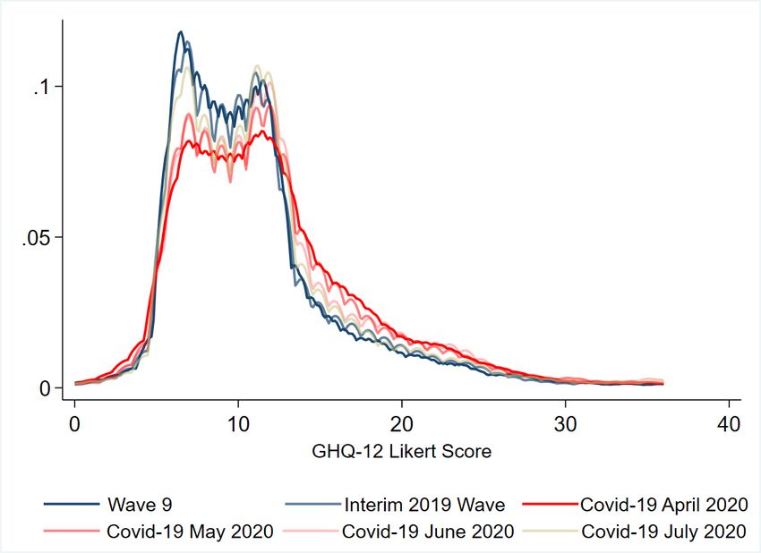
threshold value for psychological distress, increases from 0.185 at the 2019 Wave to
 0.277 in April 2020. In other words, on this measure, just under 20% of the sample were
 experiencing psychological distress in 2019, but by April 2020, almost 30% of the same
 sample of individuals were experiencing distress. These levels of psychological distress
 move back towards pre-pandemic levels by the July 2020 COVID-19 Wave (collected
 after the almost complete easing of the first lockdown) but the worsening in GHQ scores,
 relative to 2019, remains statistically significant for many of them including the
 aggregate scores.

 Table 1: Summary statistics for the GHQ.
 Wave 9 Interim April May 2020 June July
 2019 2020 2020 2020
Panel A: Sample proportions and means
 GHQ-12 elements†
 Concentration 0.154 0.162 0.274¶ 0.246¶ 0.239¶ 0.177¶
 Sleep 0.142 0.148 0.236¶ 0.198¶ 0.202¶ 0.157
 Role 0.126 0.129 0.272¶ 0.236¶ 0.211¶ 0.161¶
 Decisions 0.086 0.090 0.131¶ 0.128¶ 0.139¶ 0.108¶
 Strain 0.220 0.219 0.282¶ 0.260¶ 0.260¶ 0.211¶
Overcoming difficulties 0.124 0.130 0.140 0.142¶ 0.155¶ 0.127
 Enjoy activities 0.160 0.168 0.462¶ 0.417¶ 0.373¶ 0.278¶
 Face up problems 0.094 0.098 0.124¶ 0.120¶ 0.131¶ 0.105
 Depressed 0.184 0.196 0.270¶ 0.255¶ 0.237¶ 0.201
 Confidence 0.147 0.156 0.158 0.175¶ 0.174¶ 0.154
 Worthlessness 0.078 0.082 0.090 0.096¶ 0.101¶ 0.085
 Happiness 0.142 0.148 0.231¶ 0.205¶ 0.200¶ 0.171¶
 GHQ-12 Likert‡‡ 11.07 11.22 12.30¶ 12.25¶ 12.36¶ 11.65¶
GHQ-12 Caseness ≥4‡‡‡ 0.171 0.185 0.277¶ 0.257¶ 0.245¶ 0.201¶
Panel B: Overall inequality measure (GHQ-12 Likert‡‡)
 Variance 29.23 29.61 35.50¶ 35.19¶ 37.32¶ 31.68
 MLD index 0.101 0.100 0.112 ¶ 0.108 ¶ 0.109¶ 0.101
 Sample size 8,222 8,185 7,512 7,025 6,786 6,642
Notes: Results in the first two columns (wave 9 and interim 2019 wave) use the UKHLS Wave 9 sample
weights while those in the third-sixth columns are weighted by using our own longitudinal weights.
† For each of the GHQ dimensions, the two categories indicating the most depressed states are coded as one

and the remaining two categories, that reflect better mental health, are coded as zero (dichotomous variables).
‡‡ Continuous GHQ-12 measure based on the overall score across all 12 dimensions using the Likert scoring

(ranging between zero and 36).
‡‡‡ Dichotomous variable taking the value of one if the overall GHQ-12 Caseness score ≥4 and zero otherwise.
¶ Comparison between the Interim 2019 Wave and the COVID-19 waves: differences in the mean values (or

variance) compared to the corresponding results at Interim 2019 Wave are statistically significant at least at
the 5% level.

 Panel B of Table 1 compares total inequality for the Likert GHQ-12 score, measured by
 the variance and the MLD index, before and during the pandemic. Differences in
 inequality measures between Wave 9 and the 2019 Wave are not statistically
 significant, suggesting the absence of systematic differences in the level of inequality in
 psychological distress during the immediate period before the onset of the pandemic.
 However, there is a systematic and statistically significant increase in total inequality
 from baseline to the COVID-19 waves; for example, the variance of the GHQ-12 Likert
 score increases from 29.61 at the 2019 Wave to 35.51 in April and up to 37.32 in June
 2020. Figure 1 shows the change in the shape of the, kernel smoothed, density function

 12

for GHQ-12 between Wave 9, the 2019 Wave, and the COVID waves, with a flattening of
the density and greater mass in the right-hand tail of the distribution.

 Figure 1: Distribution of GHQ-12 Likert score at UKHLS Wave 9, Interim 2019 Wave
 and COVID-19 Waves.

Our analysis so far shows an increase in the total inequality in GHQ during the first
wave of the pandemic, but does the same hold for observed socioeconomic inequality? To
assess this, Table 2 presents the dissimilarity indices for socioeconomic inequality in
each of the twelve elements of the GHQ. The baseline results for the restricted Wave 9
sample (conditional on responding to the COVID-19 GHQ questionnaire) range between
0.223 and 0.346; the corresponding results for the 2019 Wave are similar and no
systematic differences are observed in the dissimilarity indexes between Wave 9 and the
2019 Wave (p-values>0.10, Table 2). Regarding the COVID-19 waves, the estimated
dissimilarity indices are smaller in magnitude for all but one of the twelve elements of
the GHQ in April 2020 (the exception is confidence). Formal tests for the differences in
dissimilarity indexes between the 2019 Wave and the COVID-19 waves show that the
reduction in socioeconomic inequality is statistically significant for some elements of the
GHQ-12 questionnaire; for example, the dissimilarity index for limited enjoyment of
day-to-day activities decreases from 0.236 at Wave 9 and in 2019 to values in the range
0.086-0.154 for the COVID-19 waves. Dissimilarity indexes revert towards the pre-
pandemic levels in July (following the easing of the first lockdown) but in some cases

 13

there is still systematically lower observed socioeconomic inequality compared to the
 baseline. Overall, these results indicate that the proportion of total inequality attributed
 to our observed circumstances factors did not increase during the first wave of the
 pandemic (April-July 2020).

 Table 2: Measures of socioeconomic inequality (Dissimilarity Indices) for each element of
 the GHQ.
 Wave 9 Interim April May June July
 2019 2020 2020 2020 2020

GHQ-12 elements
(Dissimilarity Indices)
 0.245*** 0.242*** 0.218*** 0.211*** 0.216*** 0.242***
Concentration (0.009) (0.010) (0.012) (0.011) (0.013) (0.011)
 Difference to 2019 wave [p-values]† 0.753 ─ 0.155 0.043 0.074 0.925
 0.243*** 0.229*** 0.219*** 0.216*** 0.204*** 0.233***
Sleep 
 (0.009) (0.009) (0.011) (0.011) (0.011) (0.010)
 Difference to 2019 wave [p-values]† 0.380 ─ 0.545 0.449 0.109 0.776
 0.271*** 0.268*** 0.174*** 0.204*** 0.221*** 0.220***
Role 
 (0.010) (0.009) (0.010) (0.011) (0.010) (0.010)
 Difference to 2019 wave [p-values]† 0.889 ─ 0.000 0.000 0.000 0.008
 0.289*** 0.288*** 0.246*** 0.273*** 0.265*** 0.264***
Decisions 
 (0.008) (0.009) (0.009) (0.010) (0.011) (0.009)
 Difference to 2019 wave [p-values]† 0.992 ─ 0.043 0.469 0.222 0.220
 0.233*** 0.230*** 0.218*** 0.218*** 0.223*** 0.226***
Strain 
 (0.010) (0.010) (0.012) (0.012) (0.011) (0.011)
 Difference to 2019 wave [p-values]† 0.774 ─ 0.324 0.334 0.608 0.799
 0.308*** 0.295*** 0.252*** 0.278*** 0.266*** 0.276***
Overcoming difficulties 
 (0.010) (0.010) (0.010) (0.010) (0.011) (0.010)
 Difference to 2019 wave [p-values]† 0.414 ─ 0.016 0.363 0.103 0.349
 0.236*** 0.237*** 0.086*** 0.089*** 0.117*** 0.154***
Enjoy activities 
 (0.009) (0.009) (0.012) (0.012) (0.011) (0.011)
 Difference to 2019 wave [p-values]† 0.989 ─ 0.000 0.000 0.000 0.000
 0.297*** 0.297*** 0.270*** 0.277*** 0.287*** 0.276***
Face up problems 
 (0.009) (0.009) (0.010) (0.010) (0.011) (0.010)
 Difference to 2019 wave [p-values]† 0.996 ─ 0.168 0.334 0.604 0.785
 0.223*** 0.207*** 0.177*** 0.195*** 0.208*** 0.211***
Depressed 
 (0.010) (0.010) (0.011) (0.012) (0.013) (0.012)
 Difference to 2019 wave [p-values]† 0.224 ─ 0.024 0.383 0.916 0.785
 0.270*** 0.255*** 0.275*** 0.259*** 0.257*** 0.255***
Confidence 
 (0.010) (0.010) (0.010) (0.011) (0.011) (0.011)
 Difference to 2019 wave [p-values]† 0.352 ─ 0.237 0.822 0.927 0.974
 0.346*** 0.368*** 0.309*** 0.339*** 0.305*** 0.312***
Worthlessness 
 (0.009) (0.009) (0.010) (0.010) (0.010) (0.009)
 Difference to Wave 9 [p-values]† 0.274 ─ 0.013 0.197 0.002 0.016
 0.257*** 0.245*** 0.165*** 0.197*** 0.229*** 0.231***
Happiness 
 (0.009) (0.009) (0.011) (0.011) (0.011) (0.011)
 Difference to 2019 wave [p-values]† 0.466 ─ 0.000 0.000 0.283 0.375
Note: Results in the first two columns (Wave 9 and the Interim 2019 Wave) use the UKHLS sample weights while those in
the third-sixth columns are weighted by using our own longitudinal weights. Bootstrapped standard errors for the
inequality measures in parenthesis (500 replications).
 ***p < 0.01 (for the Ho hypothesis that the dissimilarity index is equal to zero)
† Test for differences in the inequality measures compared to the corresponding results for the Interim 2019 Wave;

bootstrapped p-values using 500 replications.

 14

Table 3, Panel A presents the measures for the variance share (and the MLD index
share) for our composite GHQ-12 Likert measure that show the fraction of the total
inequality in the GHQ-12 Likert measure that is attributed to the observed
socioeconomic inequality. The baseline results for the 2019 Wave are statistically
significant with observed circumstances accounting for 12.82% for the total variance in
GHQ-12 (14.53% for the MLD index). These values fall to 11.12% (11.52% for the MLD
index) in April 2020, and this reduction is statistically significant, showing that
circumstances account for a smaller share of total inequality and that relative
socioeconomic inequality did not increase during the peak of the pandemic. Similar
patterns are observed in the May-July Waves. Figure 2 shows that despite the increase
in the absolute total variance (total inequality) in the Likert GHQ-12 composite score
(also shown in Table 1, Panel B), the absolute explained variance has remained stable,
hence the fall in the variance share (i.e., to the proportion of the total inequality
attributed to observed circumstances). Overall, these results show that relative
socioeconomic inequality did not increase during the peak of the pandemic. Results from
the dissimilarity indexes for the caseness score are similar; there are no systematic
differences in dissimilarity indexes between Wave 9 and the 2019 Wave, while
dissimilarity indexes are lower during the first wave of the pandemic.

To explore the extent of the potential role of non-response and sample selection bias in
our inequality results we also estimated our inequality measures without accounting for
sample weights (full results are available in Tables C.4.-C.6., Appendix C)15. Overall, we
find that our inequality results are comparable with and without accounting for weights
and, thus, the potential role of the non-response and selection bias seems not to affect
our main conclusions. Specifically, we find that without accounting for sample weights
our inequality measures are reduced by around 10 percentage points compared to the
base case results (Tables 2 and 3); this highlights the presence of a modest
underestimation of inequality when we do not adjust for non-response. One may argue
however that restriction of our baseline sample (Wave 9 and Interim Wave) to those who
ever completed a COVID-19 survey may impose further biases to our analysis that are
not adequately addressed using our sample weights. Estimation of our inequality and
decomposition results based on the non-restricted Wave 9 sample shows practically
identical results to the corresponding results for the Wave 9 sample presented in the
main text of the paper (results available upon request)16.

15 Summary statistics (Table B.1.) show that the mean values of the pre-existing circumstance
(Waves 1-8) are similar between the baseline Wave 9/Interim Wave sample and the subsequent
COVID-19 waves (columns b-f). This suggests that our longitudinal sample weights are relevant
in achieving a good balance in the mean value of the pre-existing circumstances in COVID-19
waves (compared to baseline) and, thus, they may provide good adjustments for non-response
biases.
16 As a further reassurance the comparison of the mean values for the pre-existing circumstance

variables between the full Wave 9 and the restricted Wave 9 sample show limited differences
(Table B.1. columns a and b).

 15

Table 3: Measures of socioeconomic inequality for levels of GHQ-12 (Likert scoring) and
 for dichotomous distress indicators.
 Wave 9 Interim April May June July
 2019 2020 2020 2020 2020
 Panel A. GHQ-12 Likert

Relative inequality: 12.11*** 12.82*** 11.12*** 12.33*** 12.26*** 10.87***
Variance share (0.413) (0.449) (0.355) (0.415) (0.423) (0.400)
 Difference to 2019 wave†
 0.110 ─ 0.000 0.336 0.240 0.000
 [p-value]
Relative inequality: 13.99*** 14.53*** 11.52*** 13.26*** 13.47*** 12.49***
MLD index share (0.360) (0.364) (0.269) (0.340) (0.362) (0.339)
 Difference to 2019 wave†
 0.371 ─ 0.000 0.001 0.007 0.000
 [p-value]
 Panel B. GHQ-12 Caseness≥4

 0.262*** 0.241*** 0.203*** 0.211*** 0.211*** 0.228***
Dissimilarity index 
 (0.010) (0.010) (0.011) (0.011) (0.011) (0.011)
 Difference to 2019 wave†
 0.129 ─ 0.004 0.010 0.010 0.403
 [p-value]
Note: Results in the first two columns (Wave 9 and Interim 2019 Wave) use the UKHLS sample weights while
those in the third-sixth columns are weighted by using our own longitudinal weights. Bootstrapped standard
errors for the inequality measures in parenthesis (500 replications).
 ***p < 0.01 (for the Ho hypothesis that the inequality measure is equal to zero).
† Test for differences in the inequality measures compared to the corresponding results for the Interim 2019

Wave; bootstrapped p-values using 500 replications.

 Figure 2: Total and explained variance of GHQ-12 Likert score.

 16

4.2 Decomposition analysis
Table 4 presents the Shapley-Shorrocks decomposition of the variance share for our
composite Likert GHQ-12 measure (Figure 3 presents an overview graphically). Table
B.2 (Appendix B) presents the corresponding Shapley-Shorrocks decomposition results
for the dissimilarity indices for the GHQ-12 caseness score; these results echo those in
Table 4. Our results show the detailed contribution of each of our age-gender categories
and are grouped by categories of the other circumstance variables: ethnicity, education,
housing conditions, household composition, employment status, industry, income,
neighbourhood, parental occupation, and chronic conditions. Before the pandemic, in
Wave 9 and the 2019 Wave, the largest contributions to socioeconomic inequality are
those attributed to chronic conditions (about 32%), housing conditions (18-20%) and
employment status (15-16%). In contrast, during the peak of the first wave of the
pandemic (April 2020) these three factors decline in their relative shares and
demographic factors (age and gender) account for the largest share, increasing their
share from 15% to 33%, with most notable increase for younger women. The
contribution of working in an industry relevant to the response to the pandemic plays a
small role at the 2019 Wave (1.05%), but nearly triples its share in April 2020 (2.68%).

Table 4: Decomposition of relative socioeconomic inequality in GHQ-12 (variance share).
 Wave 9 Interim April May June July
 2019 2020 2020 2020 2020
 GHQ-12 (Variance share) % % % % % %
 Males 35-49 0.23 0.30 1.39 0.41 0.41 0.43
 Males 50-64 1.10 1.85 5.73 3.46 3.02 3.20
 Males 65+ 7.14 6.30 10.16 8.86 8.01 9.80
 Females 20-34 2.13 1.80 9.56 4.71 2.53 1.56
 Females 35-49 1.76 2.63 4.39 3.05 3.40 3.69
 Females 50-64 0.78 0.64 1.16 0.78 0.64 0.78
 Females 65+ 1.96 1.76 1.14 0.99 0.92 1.02
 Age and gender total 15.1 15.28 33.53 22.26 18.93 20.48
 Ethnicity 0.92 0.38 1.40 0.98 1.34 1.94
 Education/qualifications 0.63 0.59 0.76 1.86 1.32 1.72
 Housing conditions 18.41 20.21 14.35 21.48 16.46 16.62
 Household composition 5.58 5.12 6.36 7.50 6.61 3.62
 Employment status 15.86 15.33 11.45 11.93 10.53 10.65
 COVID19-related industry 0.86 1.05 2.68 2.04 1.73 3.39
 Income 3.90 3.70 1.16 2.64 2.97 2.12
 Neighbourhood characteristics 4.59 4.59 4.85 6.78 5.32 10.07
 Parental occupational status 1.20 1.43 2.81 1.33 1.45 2.48
 Chronic conditions 32.95 32.31 20.65 21.18 33.35 26.93
 Total 100.00 100.00 100.00 100.00 100.00 100.00
 Notes: Results in the first two columns (Wave 9 and Interim 2019 Wave) use the UKHLS sample weights
 while those in the third-sixth columns are weighted by using our own longitudinal weights.

 Figure 3: Decomposition analysis of GHQ-12 Likert scores.

 17

Note: Factor’s contributions are ordered according to their contributions at April 2020 COVID
Wave.

As the first wave of the pandemic progressed, the contribution of demographics dropped
from the peak levels of April and the contribution of other factors, such as chronic health
conditions, housing conditions, household composition and neighbourhood
characteristics have begun to explain a larger share. These results are in line with other
evidence that has shown a strong demographic gradient on how the pandemic affects the
mental health of the population, especially among younger women (Banks and Xu,
2020). They also reveal the increasing role of other socioeconomic circumstances as
sources of stress during the COVID-19 outbreak. For example, household composition
shows an increasing contribution (May and June 2020) which may capture loneliness
among single-person households during the lockdown and the anxiety associated with
the higher risks of COVID-19 transmission for multi-generational and multi-occupied
households (Haroon et al., 2020).

To provide further evidence on the role of our circumstances variables (and as a way
explore the robustness of our results) we estimate regression models on the continuous
Likert GHQ-12 during the peak of the first wave of the COVID-19 (April 2020)
separately for the sub-samples of those with and without psychological distress at the
baseline (using the binary GHQ-12 Caseness≥4 indicator). Table B.3 (Appendix)
presents Shapley decomposition of the contribution of circumstance variables to
explained variance of the continuous Likert GHQ-12 score (i.e., the model R-squared).

 18

Overall, these results confirm the dominant role of age and gender as they account for
more than 45% of the explained variance in the GHQ-12 scores for those who did not
experience psychological distress at baseline; in particular this suggests that
demographics play an important role in worsening mental health during the peak of the
pandemic. The corresponding percentage contribution for demographics is much less
evident for the case of those already experienced mental health issues at baseline.
Moreover, of particular relevance for our inequality decomposition results, income itself
seems not to exert notable contributions, while housing conditions and chronic
conditions have the largest contributions in explaining GHQ Likert outcomes for those
with and without cases of psychological distress at the baseline.

5 Conclusion
The UK population as a whole has been exposed to the policy responses to the COVID-
19 pandemic. Measures taken include a lockdown, social distancing and self-isolation.
Their economic impact has been substantial and resources within the health and social
care systems have been diverted to the pandemic. Given evidence that the impact of the
pandemic on physical health and mortality has been more severe for those in
disadvantaged circumstances (e.g., Office for National Statistics, 2020a) it might
reasonably be expected that the impact on psychological distress and the mental health
of the population may also have been unequally distributed within the population.

In line with the evidence on physical health, our results show a substantial worsening of
the overall levels of GHQ during the peak (of the first wave) of the pandemic. This
applies to nearly all of the individual elements of GHQ-12 and to overall GHQ-12 scores.
In addition, there is a statistically significant increase in total inequality in the Likert
GHQ-12 score between the periods before (Wave 9 and the 2019 Wave) and during the
pandemic (April-July 2020). Nevertheless, we find that the proportion of the total
inequality that is attributed to our observed set of pre-existing socioeconomic
circumstances did not increase during the first wave of the pandemic. Our results
suggest that, with respect to psychological distress, the greater total inequality that is
evident, is broadly diffused across the population. This is consistent with the notion that
the first wave of the pandemic was, to some extent, a leveller as far as pre-existing
circumstances are considered. For example, recent evidence from the USA shows that
individuals with higher socioeconomic status experienced a greater increase in
depressive symptoms and a decrease in life satisfaction during COVID-19 in comparison
to those with lower socioeconomic status (Wanberg et al., 2020). However, it should be
noted here that greater unexplained variation may prove challenging for policy makers
and it will be interesting to see whether this finding persists in future waves of the
pandemic.

The Shapley-Shorrocks decomposition analysis of the shares of inequality that are
attributable to observed circumstances shows that during the peak of the pandemic
(April 2020), key socioeconomic factors declined in their share of socioeconomic

 19