DESCRIPTION OF THE REMIND R MODEL - POTSDAM INSTITUTE FOR ...
←
→
Page content transcription
If your browser does not render page correctly, please read the page content below
Description of the ReMIND‐R model
Description of the ReMIND‐R model
– Version June 2011 –
Gunnar Luderer, Marian Leimbach, Nico Bauer, Elmar Kriegler12
1 Overview
This model description is based on the introduction of the REMIND‐R model in Leimbach et al.
(2009), as well as the technical description in Bauer et al. (2008) and Bauer et al. (2010). More
information is also available from the ReMIND‐website3.
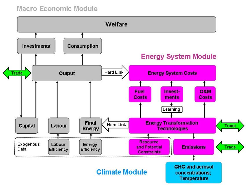
ReMIND‐R is a global energy‐economy‐climate model. Figure 1 provides an overview of the
general structure of ReMIND‐R. The macro‐economic core of ReMIND‐R is a Ramsey‐type
optimal growth model in which intertemporal global welfare is optimized subject to equilibrium
constraints. It considers 11 world regions and explicitly represents trade in final goods, primary
energy carriers, and, in the case of climate policy, emission allowances. It is formulated such
that it yields a distinguished Pareto‐optimal solution which corresponds to the market
equilibrium in the absence of non‐internalized externalities. For macro‐economic production,
capital, labor and energy are considered as input factors. The macro‐economic output is
available for investment into the macro‐economic capital stock, consumption, trade, and costs
incurred from the energy system.
The macro‐economic core is hard‐linked to the energy system module. Economic activity results
in demand for final energy such as transport energy, electricity, and non‐electric energy for the
stationary end‐uses. The demand for final energy is determined via nested constant elasticity of
substitution (CES) production function (cf. Section 2.1). The energy system module considers
endowments of exhaustible primary energy resources as well as renewable energy potentials. A
substantial number (~50) of technologies are available for the conversion of primary energies to
secondary energy carriers. Moreover, capacities for transport and distribution of secondary
energy carriers for final end use are represented. The costs for the energy system, including
investments into capacities, operation and maintenance costs as well as extraction and fuel
1
All authors are affiliated with the Postdam Institute for Climate Impact Research, Potsdam, Germany
2
Further members of the ReMIND‐R Team include: Lavinia Baumstark, Christoph Bertram, Tabare Curras, Anastasis
Giannousakis, Markus Haller, David Klein, Theresa Lenz, Sylvie Ludig, Michael Lüken, Ioanna Mouratiadou, Robert
Pietzcker, Franziska Piontek, Jana Schwanitz, Jessica Strefler, Falko Ueckerdt, Ottmar Edenhofer
3
At http://www.pik‐potsdam.de/research/research‐domains/sustainable‐solutions/remind‐code‐1 the technical
description of REMIND‐R is available. REMIND‐R is programmed in GAMS.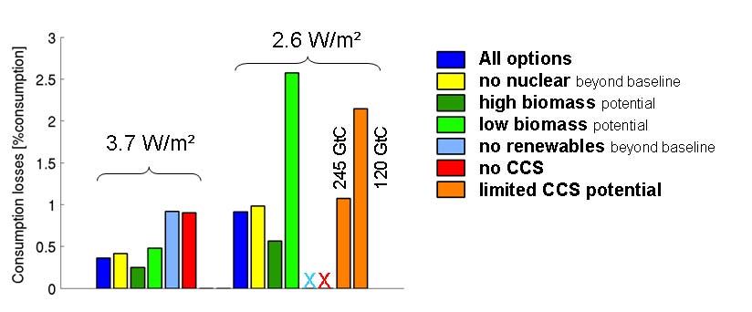
Description of the ReMIND‐R model

costs appear in the macroeconomic budget function, thus reducing the amount of economic
output available for consumption.

The model system also includes a climate module. In addition to CO2 emissions from the
combustion of fossil fuels, other greenhouse gas emissions are determined via marginal
abatement costs curves or by assuming exogenous scenarios. A rather simple reduced form
climate model is used in the current version of ReMIND‐R (cf. Section 4). The integration of the
more complex climate module ACC2 (Tanaka and Kriegler, 2007) is under way, but its
deployment is subject to computational constraints.

   Figure 1: Overall structure of the ReMIND‐R model

In particular in terms of its macro‐economic formulation, REMIND‐R resembles well‐known
energy‐economy‐climate models like RICE (Nordhaus and Yang, 1996) and MERGE (Manne et
al., 1995; Kypreos and Bahn, 2003). REMIND‐R is distinguished from these models by a high
technological resolution of the energy system and intertemporal trade relations between
regions. This results in a high degree of where‐flexibility (abatement can be performed where it
is cheapest) and what‐flexibility (optimal allocation of abatement among end‐use sectors) for
the mitigation effort
Description of the ReMIND‐R model

Table 1 provides an overview of the key features of the model. The individual modules along
with relevant parameters and assumptions are described in more detail in the following
sections.

key distinguishing                                         ReMIND‐R
feature
Macro‐economic core and      Intertemporal optimization: Ramsey‐type growth model, Negishi
solution concept             approach for regional aggregation
Expectations/Foresight       Default: perfect foresight.
Substitution possibilities   Nested CES function for production of generic final good from basic
within the macro‐            factors capital, labor, and different end‐use energy types
economy / sectoral
coverage
Link between energy          Economic activity determines demand; energy system costs
system and macro‐            (investments, fuel costs, operation and maintenance) are included in
economy                      macro‐economic budget constraint. Hard link, i.e. energy system and
                             macro‐economy are optimized jointly.
Production function in the   Linear substitution between competing technologies for secondary
energy system /              energy production. Supply curves for exhaustibles (cumulative
substitution possibilities   extraction cost curves) as well as renewables (grades with different
                             capacity factors) introduce convexities.
Land use                     MAC curves for deforestation
International macro‐         Single market for all commodities (fossil fuels, final good, permits)
economic linkages / Trade
Implementation of climate    Pareto‐optimal achievement of concentration, forcing or temperature
policy targets               climate policy targets under full when‐flexibility. Allocation rules for
                             distribution of emission permits among regions.
                             Other options: Emission caps & budgets, taxes equivalent.
Technological Change /       Learning by doing (LbD) for wind and solar. A global learning curve is
Learning                     assumed. LbD spillovers are internalized. Labor productivity and
                             energy efficiency improvements are prescribed exogenously.
Representation of end‐use    Three energy end‐use sectors: Electricity production, stationary non‐
sectors                      electric, transport
Cooperation vs. non‐         Pareto: full cooperation
cooperation
Discounting                  Constant rate of pure time preference (3%)
Investment dynamics          Capital motion equations, vintages for energy supply technologies,
                             adjustment costs for acceleration of capacity expansion in the energy
                             system

    Table 1: Overview of key characteristics of the ReMIND‐R model.
Description of the ReMIND‐R model
2 The Macro-Economic Kernel and Solution Concept
REMIND‐R as introduced by Leimbach et al. (2009) is a multi‐regional hybrid model which
couples an economic growth model with a detailed energy system model and a simple climate
model. The hard‐link between the energy system and the macroeconomic system follows the
method by Bauer et al. (2008). Assuming perfect foresight and aiming at welfare maximization,
REMIND‐R simulates the world‐economic dynamics over the time horizon 2005 to 2150 with a
time step of five years. In order to avoid distortions due to end‐effects, our analysis focuses on
the results for the time span 2005‐2100.
In its present version, ReMIND‐R distinguishes 11 world regions (Figure 2):
USA ‐ USA
EUR ‐ EU27
JAP ‐ Japan
CHN ‐ China
IND ‐ India
RUS ‐ Russia
AFR ‐ Sub‐Saharan Africa (excl. Republic of South Africa)
MEA ‐ Middle East, North Africa, central Asian countries
OAS ‐ Other Asia (mostly South East Asia)
LAM ‐ Latin America
ROW ‐ Rest of the World (Canada, Australia, New Zealand, Republic of South Africa,
Rest of Europe).
Figure 2: ReMIND‐R region definitions.Description of the ReMIND‐R model
2.1 Objective function and production structure
Each region is modeled as a representative household with a utility function that depends upon
per capita consumption:
C
U r e ρt Lrt log rt ,
t Lrt
where Lt and Ct are population and consumption and time t, respectively. Utility calculation is
subject to discounting. We assume a pure rate of time preference of 3 %. The logarithmic
functional relation between per‐capita consumption and utility implies an elasticity of marginal
consumption of 1. Thus, in line with the Keynes‐Ramsey‐Rule, ReMIND‐R yields an endogenous
interest rate in real terms of 5‐6% for an economic growth rate of 2‐3%. This is well in line with
interest rates typically observed on capital markets.
It is the objective of REMIND‐R to maximize a global welfare function that results as a weighted
sum of the regional utility functions:
W nr U r .
r
The weights nr (also called Negishi weights) are chosen such that the sum of the discounted
value of exports equals that of the imports over the time horizon considered. Numerically, this
clearing of each region’s intertemporal trade balance is achieved via an iterative algorithm. It
ensures that the Pareto‐optimal solution of the model corresponds to the market equilibrium in
absence of non‐internalized externalities (cf. Section 2.2).
Marco‐economic output, i.e. gross domestic product (GDP), of each region is determined by a
"constant elasticity of substitution" (CES) function of the production factors labor, capital and
end use energy. The end use energy of the upper production level is calculated as a production
function which comprises transportation energy and stationary used energy. Both are
connected by a substitution elasticity of 0.3. These two energy types are in turn determined by
means of nested CES functions of more specific final energy types (see Figure 3). Substitution
elasticities between 2.5 and 3 hold for the lower levels of the CES nest. An efficiency parameter
is assigned to each production factor in the various macroeconomic CES functions. Changes in
the efficiency of the individual production factors for each region are given by exogenous
scenarios.Description of the ReMIND‐R model Figure 3: Production structure of ReMIND. The conversion of primary energy (lowest level) to secondary energy is represented in the energy system module based on linear production functions. Aggregation of secondary energy to final energy carriers and aggregated macro‐ economic energy input is represented via nested CES structures. In each region, produced GDP Y(t) is used for consumption C(t), investments into the macroeconomic capital stock I(t), energy system expenditures and for the export of composite goods XG. Energy system expenditure consist of fuel costs GF(t), investment costs GI(t) and operation & maintenance costs GO(t). Imports of the composite good MG increase the available GDP: This balance of GDP distribution forms the budget constraint each region is subjected to. Macroeconomic investments enter a conventional capital stock equation with an assumed depreciation rate of 5 %.
Description of the ReMIND‐R model
2.2 Trade
In following the classical Heckscher‐Ohlin and Ricardian models (Flam and Flanders, 1991),
trade between regions is induced by differences in factor endowments and technologies. In
ReMIND‐R, this is supplemented by the possibility of intertemporal trade. However, there is no
bilateral trade, but exports in and imports from a common pool. Trade is modeled in the
following goods:
Coal
Gas
Oil
Uranium
Composite good (aggregated output of the macro‐economic system)
Permits (emission rights), in the case of climate policy
Intertemporal trade and the capital mobility implied by trade in the composite good cause
factor price equalization and provide the basis for an intertemporal and interregional
equilibrium.
In REMIND‐R, the balance between exports and imports for each kind of goods in each period is
guaranteed by adequate trade balance equations. However, the question whether a chosen
trade structure is intertemporally balanced and optimal depends on how the welfare weights
are adjusted. A distinguished Pareto‐optimal solution, which in the case of missing externalities
also corresponds to a market solution, can be obtained by adjusting the welfare weights
according to the intertemporal trade balances.
The intertemporal budget constraint each region is subject to means that each composite
goods export qualifies the exporting region for a future import (of the same present value), but
implies for the current period a loss of consumption. Trade with emission permits works in a
similar way. In the default setting, the presence of a global carbon market is assumed: Initial
allocation of emission rights are determined by a burden sharing rule, and permits can be
traded freely among world regions. A permit constraint equation ensures that each unit of CO2
emitted by combusting fossil fuels is covered by emission certificates.
The representative households in REMIND‐R are indifferent regarding domestic and foreign
goods as well as indifferent among foreign goods of different origin. This can potentially lead to
a strong specialization and, related to the cooperative setting implied by the solution concept,
to rather optimistic results. For climate policy assessments this is less critical as it applies to
both baseline and policy scenarios.Description of the ReMIND‐R model
2.3 Climate policy analysis
The ReMIND model is usually run in two modes.
A “business as usual” mode in which the global welfare function is optimized
without constraints. This resembles a situation where the occurrence of climate
change would have no effect on the economy and the decisions of the
representative households in the regions.
A “climate policy” mode where an additional climate policy constraint is imposed on
the welfare optimization. The constraint can take the form of a limit on
temperature, forcing (from Kyoto gases or all radiative substances), CO2
concentration, cumulative carbon budget, or CO2 emissions over time. The
mitigation costs of reaching the policy goal to meet the climate constraint is
calculated as percentage reduction of net present value consumption or GDP w.r.t.
to the business as usual case.
The impact of a pre‐specified carbon tax can also be studied in ReMIND, although it is less
straightforward. For such scenarios, the tax is implemented as a penalty on emissions. This tax
as part of each region’s budget constraint is counterbalanced by an fixed amount of tax
revenues. The model is solved iteratively with adjusted tax revenues until these match the tax
payments.
3 The energy system
The energy system module (ESM) of ReMIND‐R comprises a detailed description of energy
carriers and conversion technologies. The ESM is embedded into the macroeconomic growth
model: the techno‐economic characteristics and the system of balance equations that set up
the energy system are constraints to the welfare maximization problem of the macroeconomic
module.
The energy system can be regarded as an economic sector with a heterogenous capital stock
that demands primary energy carriers and supplies secondary energy carriers. The structure of
the capital stock determines the energy related demand‐supply structure. The macro‐economy
demands final energy as an input factor for the production of economic output. In return, the
energy sector requires financial resources from the capital market that are allocated among a
portfolio of alternative energy conversion technologies. The techno‐economic characteristics of
the technologies and endogenously evolving prices of energy and CO2 emissions determine the
size and structure of the energy sector capital stock. Hence, the energy sector develops
according to an equilibrium relationship to the remaining economy with which it is interrelated
through capital and energy markets.Description of the ReMIND‐R model
3.1 Primary energy resources
The primary energy carriers available in the ESM include both exhaustible and renewable
resources:
Coal
Oil
Gas
Uranium
Hydro
Wind
Solar
Geothermal
Biomass
The exhaustible resources (coal, oil, gas and uranium) are characterized by extraction costs that
increase over time as cheaply accessible deposits become exhausted. In ReMIND‐R, this is
represented via region‐specific extraction cost curves which prescribe increasing costs of
production with increasing cumulative extraction. In addition, adjustment costs are applied that
represent short‐term price markups in case of rapid expansion of resource production. While
resources are assumed to be tradable across regions, resource trade is subject to region and
resource‐specific trade‐costs.
By contrast, renewable energy sources do not deplete over time. They are represented via
region‐specific potentials. For each renewable energy type, the potentials are classified into
different grades, each of which is characterized by a specific capacity factor. Superior grades
feature high capacity factors and will produce more energy for a given installed capacity, while
inferior grades will have lower yields. As a result of the optimization, this grade structure leads
to a gradual expansion of renewable energy deployment over time.
The potentials for solar PV and CSP are based on DLR (2009). To account for the competition of
PV and CSP for certain sites, an additional constraint for the combined deployment of PV and
CSP was introduced (Pietzcker et al., 2009). The total solar potential is as high as 10 000 EJ/yr,
with almost half of it located in Africa.
Global potentials for onshore wind are assumed to be 120 EJ/yr. This value is twice the
potential estimated by WBGU (2003), and about half that given by De Vries et al. (2006).
Regional disaggregation is based on Hoogwijk (2004). An additional resource potential of 40 EJ
was assumed for offshore wind. Since offshore wind is not represented explicitly in the present
version of ReMIND‐R, the offshore wind potential was added to the potential for conventional
wind energy, albeit at an investment cost penalty of 50%.Description of the ReMIND‐R model
Global potentials of hydro‐power are based on WBGU (2003) and disaggregated into regional
potentials based on Hoogwijk (2004).
3.2 Secondary energy carriers and energy conversion matrices
Secondary energy carriers considered in ReMIND‐R include:
Electricity
Heat
Hydrogen
Other liquids
Solid fuels
Gases
Transport fuel petrol
Transport fuel diesel
In the present version of ReMIND‐R, electricity is only demanded for stationary use. An
implementation of electrification of the transport sector is under way.
The most notable part of the energy system is the conversion of primary energy into secondary
energy carriers via specific energy conversion technologies. In total, some 50 different energy
conversion technologies are represented in ReMIND‐R. The energy conversion matrix in Table 2
provides an overview of the primary energy types, secondary energy types and relevant
conversion technologies between them.Description of the ReMIND‐R model
PRIMARY ENERGY CARRIERS
Exhaustible Renewable
Solar,
Ura‐ Geo‐
Coal Oil Gas Wind, Bio‐mass
nium thermal
Hydro
LWR, SPV,
Gen IV WT,
Electricity PC, IGCC DOT NGCC HDR BIGCC
Fast Hydro,
SECONDARY ENERGY CARRIERS
Reactors CSP
H2 C2H2 SMR B2H2
Gases C2G GasTR B2G
CoalHP, GasHP, BioHP,
Heat GeoHP
CoalCHP GasCHP BioCHP
Liquid B2L
C2L Refin.
fuels Bioethanol
Other
Refin.
Liquids
Solids CoalTR BioTR
Abbreviations: PC = conventional coal power plant, IGCC = integrated coal gasification combined
cycle, CoalCHP = coal combined hat power, C2H2 = coal to H2, C2G = coal to gas, CoalHP = coal
heating plant, C2L = coal to liquids, CoalTR = coal transformation, DOT = diesel oil turbine, Refin.
= Refinery, GT = gas turbine, NGCC = natural gas combined cycle, GasCHP = Gas combined heat
power, SMR = steam methane reforming, GasTR = gas transformation, GasHP= gas heating plant,
LWR = light water reactor, SPV = solar photo voltaic, WT = wind turbine, Hydro = hydro power,
HDR = hot‐dry‐rock, GeoHP = heating pump, BioCHP = biomass combined heat and power, BIGCC
= Biomass IGCC, B2H2 = biomass to H2, B2G = biogas, BioHP = biomass heating plant, B2L =
biomass to liquids, BioEthanol = biomass to ethanol, BioTR = biomass transformation
Table 2: The energy conversion matrix ‐ overview on primary and secondary energy
carriers and the available conversion technologies. Yellow colors indicate that
technologies can be combined with CCS.Description of the ReMIND‐R model Coal and biomass are highly flexible primary energy carriers since all types of secondary energy can be produced from them. Crude oil and natural gas are mainly used to produce liquids and gases. Renewable energy carriers other than biomass are well suited for the production of electricity, but they are less suited to produce other secondary energy carriers. Renewable energy sources including biomass are assumed to be non‐tradable. In the default setting, all secondary energy carriers are assumed to be non‐tradable across regions, while statistical data indicates that liquid fuels are traded globally. However, the scale of trade in refined fuels is relatively small compared to trade in crude oil. Since the ReMIND‐R model considers crude oil to be tradable the bias is limited. Secondary energy carriers are converted into final energy carriers by considering mark‐ups for transmission and distribution. Final energy is demanded by the macro‐economic sector and rewarded with equilibrium prices. Note that in the present ReMIND‐R version, the end use sectors household and industry are aggregated to the stationary sector. Hence, we distinguish the stationary and the transport sector as final energy demanding sectors. All technologies are represented in the model as capacity stocks. Since there are no constraints on the rate of change in investments, the possibility of investing in different capital stocks provides high flexibility of the technological evolution. Nevertheless, every additional energy production (either based on existing or new technologies) needs investments in capacities in advance. Moreover, the model does not allow for idle capacities. The lifetime of capacities differs between various types of technologies. Depreciation rates are quite low in the first two decades, and increase afterwards. Each region is initialized with a vintage capital stock calibrated to meet the input‐output relations given by IEA energy statistics (IEA 2007a,b). The technical transformation coefficients for new vintages are the same for all regions and assumed to be constant. However, the following modifications apply: the transformation efficiency is improved over time for fossil power generation technologies and different technology grades are considered when renewable energy sources are used. The by‐production coefficients of the combined power‐ heat technologies (CHP) have been region‐specifically adjusted to the empirical conditions of the base year. Ambitious mitigation targets typically result in substantial expansion of renewables, mostly solar and wind. Techno‐economic parameters for electricity generation from renewable energy sources are given in Table 3. Wind, solar PV and CSP feature learning by doing, i.e. specific investment costs decrease by 12, 20, 9%, respectively, for each doubling of capacity.
Description of the ReMIND‐R model

              Lifetime        Investment          Floor        Learning       Cumulative            O&M
                                 costs            costs          Rate        capacity 2005          costs

                [Years]           [$US/kW]      [$US/kW]          [%]               [GW]          [$US/GJ]

 Hydro                95                 3000              -             -                    -           4.23

 Geo                  35                 3000              -             -                    -            4.2
 HDR

 Wind                 40                 1200         883               12                  60            0.89

 SPV                  40                 4900         650               20                   5            2.33

 CSP                  40                 9000         2000               9                 0.4

Table 3: Techno‐economic characteristics of technologies based on non‐biomass renewable
energy sources. For details see Neij (2003), Nitsch et al. (2004), IEA (2007a), Junginger et al.
(2008), Lemming et al. (2008).

                           Units         Daily variation       Weekly variation     Seasonal variation

Technology                              Redox-Flow-            H2 electrolysis +
                                        batteries              combined cycle gas
                                                               turbine
                                                                                    Capacity penalty to
Efficiency                 [%]                          80                     40
                                                                                    secure supply
Storage capacity           [Hours]                      12                    160

Investment costs           [$US/kW]                   4000                   6000

Floor costs                [$US/kW]                   1000                   3000

Learning rate              [%]                          10                     10

Cumulative      capacity   [TW]                        0.7                    0.7
in 2005

Life time                  [Years]                      15                    15

Cheaper technologies                    Pump-storage hydro     Pump-storage hydro
but not included due                      & compressed air       & compressed air
to limited potential                               storage                storage

Table 4: Techno‐economic parameters of storage technologies; based on Chen et al. (2009)
and expert interviews.
Description of the ReMIND‐R model The fluctuating renewable electricity sources wind and solar PV require storage to guarantee stable supply of electricity; see Pietzcker et al. (2009). Since the techno‐economic parameters applied for CSP include the costs for thermal storage to continue electricity production at night‐ time, CSP is assumed not to require any further storage for balancing fluctuations. The approach implemented into the ReMIND model distinguishes between variations on the daily, weekly and seasonal time scale. The general idea of storage is that increasing market shares of fluctuating energy sources increase the need for storage because balancing the fluctuations becomes ever more important to guarantee stable electricity supply. The superposition of variations on the three time scales is completely represented. Daily and weekly variations are compensated by explicit installation of storage plants; the techno‐economic parameters are provided in Table 4. Seasonal variations demand a penalty on the capacity factors; i.e. a certain fraction of the capacity remains unused due to over‐supply. By 2050, the storage requirement results in a markup in investment cost of typically about 20% for wind and 30% for solar PV. Techno‐economic parameters for technologies based on exhaustible resources and biomass are listed in Table 5. A relevant mitigation option for the power sector, albeit typically somewhat less dominant than renewables, is the expansion of nuclear energy. Investment costs for nuclear power plants are set to 3000 $US/kW. In the present version, only thermal nuclear reactors are considered. The use of nuclear is largely constrained by limited competitiveness vis‐à‐vis renewable electricity sources as well as limited resource potentials for uranium. No external effects such as the risk of nuclear accidents or risks arising from nuclear waste are considered. In ReMIND‐R no hard limits are applied on the expansion of technologies. However, expansion in the deployment of technologies is subject to adjustment costs that scale with the square of the relative change in capacity additions between time steps. Emissions from fossil fuel combustion can be curbed by deploying carbon capture and storage (CCS). In ReMIND‐R CCS technologies exist both for generating electricity as well as for the production of liquid fuels, gases and hydrogen from coal. Moreover, biomass can be combined with CCS to generate net negative emissions. Such bioenergy CCS (BECCS) technologies are available for electricity generation (biomass integrated gasification combined cycle power plant), biofuels (biomass liquefaction), hydrogen, and syngas production. The sequestration of captured CO2 is represented explicitly in ReMIND‐R with costs for transportation and storage based on Bauer (2005). While the overall global CO2 storage potential is estimated to be as high as 1000 GtC, the regional potentials for the EU (50 GtC), Japan (20 GtC) and India (50GtC) constrain the deployment of CCS technologies significantly in these regions.
Description of the ReMIND‐R model

                         Life-     Investment costs           O&M costs           Conversion        Capture
                         time                                                      efficiency
                                                                                                      Rate

                        [Years]        [$US/kW]               [$US/GJ]                [%]            [%]

                                   No CCS       With      No CCS       With       No      With     With CCS
                                                CCS                    CCS       CCS      CCS
Coal        PC               55       1400       2400        2.57        5.04       45       36           90

            Oxyfuel          55                  2150                    4.32                37           99

            IGCC             45       1650       2050        3.09        4.20       43       38           90

            C2H2*            45       1264       1430        1.65        1.87       59       57           90

            C2L*             45       1000       1040        1.99        2.27       40       40           70

            C2G              45        900                   0.95                   60

Gas         NGCC             40        650       1100        0.95        1.62       56       48           90

            SMR              40        498         552       0.58        0.67       73       70           90

Biomass     BIGCC            40       1860       2560        3.95        5.66       42       31           90
            *

            BioCHP           40       1700                   5.06                 43.3

            B2H2*            40       1400       1700        5.27        6.32       61       55           90

            B2L*             40       2500       3000        3.48        4.51       40       41           50

            B2G              40       1000                   1.56                   55

Nuclear     TNR              40       3000                   5.04                 33~

Table 5: Techno‐economic characteristics of technologies based on exhaustible energy
sources and biomass (cf. Iwasaki (2003), Hamelinck (2004), Bauer (2005), MIT (2007), Ragettli,
(2007), Rubin et al. (2007), Schulz (2007), Uddin and Barreto (2007), Takeshita and Ymaij
(2008), Guel et al. (2007), Brown et al. (2009), Chen and Rubin (2009), Klimantos et al. (2009)).

Abbreviations analogous to Table 1. Technologies marked with * represent joint production processes. For these
processes, investment cost and efficiency penalties for capturing can be rather small. ~ a thermal efficiency of 33% is
assumed for thermal nuclear reactors.
Description of the ReMIND‐R model
SECONDARY ENERGY CARRIERS
Liquid Other
Electricity H2 Gases Heat Solids
Fuels liquids
Electricity ‐
SECONDARY ENERGY CARRIERS
H2 Electrolysis ‐
Gases ‐
Heat ‐
Liquid
‐
fuels
Other
‐
Liquids
Solids ‐
Table 6: Matrix for energy conversion from secondary to secondary energy carrier.
The only technology represented in ReMIND‐R for conversion from secondary energy to
secondary energy is the production of hydrogen from electricity via electrolysis (Table 6).
3.3 From secondary energy to final energy
The distribution of energy carriers to end use sectors forms the interface between the macro‐
economic module and the energy system module. ReMIND‐R distinguishes between the
stationary end‐use sector (aggregating industry and residential/buildings) and end use in the
transport sector. Secondary energy carriers available for supply in the stationary sector are
electricity, heat, solids, gases, liquids, and hydrogen. The transport sector consumes diesel,
petrol, and hydrogen. An implementation of electricity use in the transport sector is under way.
Transport and distribution of secondary energy carriers is represented via capacities that
require investments and incur costs for operation and maintenance.
In the present version of ReMIND‐R, no energy services (such as transportation service in
passenger km) are represented.Description of the ReMIND‐R model
END‐USE SECTORS
Stationary Transport
Electricity Transport and distribution
SECONDARY ENERGY CARRIERS
H2 Transport and distribution Transport and distribution
Gases Transport and distribution
Heat Transport and distribution
Diesel Transport and distribution
Petrol Transport and distribution
Other
Transport and distribution
Liquids
Solids Transport and distribution
Table 7: Matrix representing distribution of secondary energy to end‐use sectors.
4 Climate module
The present version of REMIND‐R includes a rather simple reduced‐form climate model similar
to the DICE model. The model includes an impulse‐response function with three time scales for
the carbon‐cycle, and an energy balance temperature model with a fast mixed layer and a slow
deep ocean temperature box. The carbon cycle – temperature model is amended by equations
describing the concentration and radiative forcing resulting from CH4 and N2O as well as
sulphate aerosols and black carbon (Tanaka and Kriegler, 2007; Lüken et al., 2010). The
emission of sulphates is directly linked to the combustion of fossil fuels in the energy sector.
CO2 emissions from land‐use changes as well as emissions of CH4 and N2O are calculated based
on marginal abatement costs curves (Lucas et al., 2006). The climate module determines the
atmospheric CO2 concentration and considers the impact of greenhouse gas emissions and
sulphate aerosols on the level of global mean temperature. The climate sensitivity ‐ as the mostDescription of the ReMIND‐R model
important parameter of the climate module – is set to 3.0°C. The integration of the more
complex climate module ACC2 (Tanaka and Kriegler, 2007) is under way, but its deployment is
subject to computational constraints.
REMIND
CO2 fuel combustion By source
other CO2 industry Exog.
CO2 LUC MAC
CH4 MAC
N2O MAC
CFCs Exog.
PFCs Exog.
SF6 Exog.
Montreal gases Exog.
CO Exog.
NOx Exog.
VOC Exog.
SO2 Coupled to CO2
Fossil fuel burning BC Exog. /
Fossil fuel burning OC Coupled to CO2 depending
on climate module
Biomass burning BC Exog.
Biomass burning OC Exog.
Nitrate Exog.
Mineral dust Exog.
Albedo Exog.
Table 8: Overview of the treatment of radiative forcing components in the climate
module.
5 Key strengths and caveats
Since ReMIND‐R is a hard‐linked coupled multi‐regional energy‐economy model it can fully
capture the interactions between economic development, trade, and climate mitigation policy.
The full macro‐economic integration is particularly valuable for the assessment of the regional
distribution of mitigation costs.
The central strength of ReMIND‐R is its ability to calculate first‐best mitigation strategies that
provide benchmark development pathways against which mitigation scenarios under sub‐
optimal settings can be compared. In particular, in its default setting ReMIND‐R featuresDescription of the ReMIND‐R model
full where‐flexibility due to interregional trade of goods and emission permits;
full when‐flexibility due to the intertemporal optimization and the endogenous choice of
a welfare‐optimizing emission reduction trajectory;
what‐flexibility within the energy system due to a fully integrated perspective on
primary energy endowments and end‐use demand. An improved representation of non‐
CO2 greenhouse gases is under development.
The fully integrated, hard‐linked formulation of ReMIND‐R along with the intertemporal
optimization make the model numerically very heavy. This computational complexity puts a
hard limit to the amount of detail that can be represented in the model. In particular, the
following caveats exist:
The spatial resolution of the model is limited to 11 world regions. Many relevant sub‐
scale processes, particularly in terms of infrastructure for power grids, transportation,
pipelines etc. are not resolved explicitly.
Electricity from renewables such as wind and solar is characterized by strong
fluctuations of supply. The challenge of integrating these intermittent power sources
into the grid is represented rather crudely (cf. Section 3.2).
The demand for final energy is represented via the macro‐economic production
function. This approach lacks detail on the level of energy consuming activities. Demand
side efficiency is therefore exogenously prescribed (via efficiency parameters that
change over time) or parameterized as substitution within the production system. This
approach can only to a limited extent capture the real‐world efficiency potentials (e.g.
McKinsey, 2007).
Technological change in the macro‐economic module is exogenously driven.
Consequently, climate policy relevant feedbacks from knowledge accumulation and
technological spillovers are missing.
In particular for ambitious climate policy scenarios, the availability of substantial
amounts of bioenergy is critical. Such massive up‐scaling of bioenergy production may
have strong implication for conservation and food security. An effort is underway to
soft‐couple ReMIND to the land‐use model MAgPIE (Lotze‐Campen et al., 2008), in order
to explore constraints and side‐effects to bioenergy production.Description of the ReMIND‐R model 6 Model Applications 6.1 Analysis of decarbonization pathways in an integrated framework Numerous interactions exist between climate policy, the energy system, and global macro‐ economic development. A central strength of ReMIND is the analysis of these interactions in an integrated framework. Figure 4 displays exemplary primary energy and electricity mixes as simulated by ReMIND‐R (based on Luderer et al., 2011). Leimbach et al. (2009) used ReMIND‐R to assess the interrelations of climate policy and trade. Bauer et al. (2011) presents a study of the role of renewables in mitigating climate change. In the context of the RECIPE project, a detailed analysis of the interplay of decarbonization strategies in different sectors was performed (Luderer et al., 2011). Moreover, the change of investment patterns required for a low‐carbon transition was analyzed in this study (Figure 5). (a) Primary Energy: Baseline (b) Primary Energy: Stabilization (c) Electricity: Baseline (d) Electricity: Stabilization Figure 4: Sample primary energy and electricity mixes for baseline and climate policy (carbon tax increasing exponentially at 5 % p.a. with a reference level of 30 US$/tCO2 in 2020), cf. Luderer et al. (2011).
Description of the ReMIND‐R model

(a) Baseline                              (b) 450 ppm CO2

   Figure 5: Energy system investment for baseline (a) and 450 ppm CO2 only stabilization
   scenario.

   6.2     Regional distribution of mitigation costs
While a large body of literature addresses the global costs of climate change mitigation, the
regional distribution of costs remains largely unexplored. Since ReMIND‐R is a fully coupled
energy‐economy model with explicit representation of relevant technologies, resource
endowments and trade, it is excellently suited for such an analysis.

First analyses of regional mitigation costs for different climate policy regimes were presented
by Leimbach et al. (2008). A detailed analysis performed in the context of RECIPE (Luderer et al.,
2009) shows that regional mitigation costs can depart substantially from the global mean. The
cost distribution can be decomposed into (1) differences in domestic abatement costs, (2)
effects related to shifts in trade volumes and prices of fossil energy carriers, and (3) financial
transfers in the context of a global carbon market. The first component relates to structural
differences in abatement costs and the potential for low‐carbon technologies, for instance
renewable potentials. The second component is particularly important for the large exporters
of fossil fuels, like Russia and the Middle East. The third component depends not only critically
on the international burden sharing and institutional framework, but also on the price of
carbon, which in turn depends on the stabilization target and low‐carbon technology
innovations. Based on an analysis with ReMIND, Lueken et al. (2009) showed that the portfolio
of technologies strongly influences the regional distribution of mitigation costs. A notable
conclusion is that under a restricted technology portfolio the initial allocation of emission
permits among nations has a greater influence on mitigation costs than under full availability of
all relevant low‐carbon options.
Description of the ReMIND‐R model

   6.3     Exploration of very low stabilization targets
The international community is committed to limit global warming to no more than 2°C.
Achieving this target with a high probability requires stabilizing greenhouse gases at less than
450 ppm CO2eq. As part of the ADAM model intercomparison exercise, the cost and feasibility
of an emission reduction trajectory that aims at 450 ppm CO2eq by 2100 and 400 ppm CO2eq by
2150 was explored. ReMIND, along with four other participating models, found such ambitious
mitigation pathways to be feasible, albeit contingent upon the large‐scale availability of
technologies to generate negative emissions.

The results suggest that stabilization in line with the 2°C target is feasible in terms of
technologies and moderate in costs. While a broad range of technologies are required for
climate change mitigation, very low stabilization relies particularly heavily on the availability of
Carbon Capture and Storage (CCS) in combination with biomass as options for removing carbon
from the atmosphere.

   6.4     Analysis of first-best vs. second best mitigation strategies
ReMIND is characterized by a high degree of flexibility and a large number of mitigation
options. Assuming limited global cooperation on climate change mitigation or constraining the
portfolio of mitigation options allows us to explore explicitly the increases in mitigation costs
and changes in decarbonization pathways under imperfect settings.

As part of the ADAM project Knopf et al. (2009) and Leimbach et al. (2010) assessed the cost
and achievability of climate mitigation targets under restricted technology portfolios for a 550
and 400 ppm CO2eq stabilization target (Figure 6). Similarly, in the context of the RECIPE
project, technology constraints for a 450 ppm CO2 only target were assessed (Luderer et al.,
2009). A robust conclusion across different stabilization scenarios and models is that restricting
the deployment of renewables and CCS results in a substantial increase of mitigation costs,
while limiting the expansion of nuclear power has a comparatively small effect. With increasing
stringency of the target, biomass and CCS become increasingly important. This is due to the fact
that combining bioenergy with CCS can generate negative emissions and therefore is pivotal for
low stabilization scenarios.

Further analysis performed in RECIPE addressed the consequences of a delay in the setup of an
international climate policy regime (Edenhofer et al., 2009). The study found that postponing
climate policy action beyond 2020 will render the 450 ppm CO2only unattainable. If a climate
policy regime in place by 2020, the target can be achieved, albeit at 40% higher costs than in
the case of immediate action. The analysis also showed that there is a benefit for world regions
to adopt climate policies early. For instance, the EU benefits from taking action immediately
Description of the ReMIND‐R model

while others wait until 2020, compared to a scenario in which all world regions delay action
until 2020 (Figure 7).

Figure 6: Mitigation costs for different stabilization levels and technology portfolios. Source:
ADAM project (Knopf et al., 2009).

Figure 7: Regional mitigation costs for different climate policy scenarios. Source: RECIPE
project (Luderer et al., 2009).
Description of the ReMIND‐R model

References
Bauer, N., O. Edenhofer, S. Kypreos (2008): Linking Energy System and Macroeconomic Growth
       Models. Journal of Computational Management Science 5, 95‐117.
Bauer, N. (2005): Carbon Capture and Sequestration‐An Option to Buy Time? Ph.D. thesis,
       Faculty of Economic and Social Sciences, University Potsdam, Germany.
Bauer, N., L. Baumstark, M. Leimbach (2011): The REMIND‐R Model: The Role of Renewables in
       the Low‐Carbon Transformation First‐Best vs. Second‐Best Worlds. Climatic Change,
       forthcoming.
Brown D, Gassner M, Fuchino T and Marechal F (2009): Thermo‐economic analysis for the
      optimal conceptual design of biomass gasification energy conversion systems. In Applied
      Thermal Engineering, Vol. 29, pp. 2137 – 2152.
Chen H, Cong TN, Yang W, Tan C, Li Y and Ding Y (2009): Progress in Electrical Energy Storage
      Systems: A Critical Review. In Progress in Natural Science, Vol. 19, pp. 291 – 312.
Chen C and Rubin ES (2009): CO2 Control Technology Effects on IGCC Plant Performance and
       Cost. In Energy Policy, Vol. 37, pp. 915 – 42.
Flam, H. and M.J. Flanders (eds.) (1991): Heckscher‐Ohlin Trade Theory, Cambridge,
       Massachusetts: MIT Press.
Guel T (2009): An Energy‐Economic Scenarios Analysis of Alternative Fuels for Transport. ETH‐
        Thesis No. 17888, Zürich, Switzerland.Hamelinck, C. (2004): Outlook for advanced
        biofuels. Ph.D. thesis, University of Utrecht, The Netherlands.
Hoogwijk, M.M. (2004): On the Global and Regional Potential of Renewable Energy Sources.
      Ph.D. thesis, University of Utrecht.
International Energy Agency (IEA), 2007a International Energy Agency (IEA), Energy Balances of
       OECD Countries, IEA, Paris (2007).
International Energy Agency (IEA), 2007b International Energy Agency (IEA), Energy Balances of
       Non‐OECD Countries, IEA, Paris (2007).
Iwasaki, W. (2003): A consideration of the economic efficiency of hydrogen production from
       biomass. Int. Jour. of Hydrogen Energy 28, 939‐944.
Junginger M, Lako P, Lensink S, Sark W and Weiss M. (2008): Technological learning in the
       energy sector. Scientific Assessment and Policy Analysis for Climate Change WAB
       500102 017. University of Utrecht, ECN. URL:
       http://www.rivm.nl/bibliotheek/rapporten/500102017.pdf (downloaded July 27, 2009)
Junginger, M., A. Faaji, W. Turkenburg (2005): Global Experience Curves for Wind Farms. Energy
       Policy 33, 133‐150.
Junginger, M., A. Faaij, W. Turkenburg (2004): Cost reduction prospects for off‐shore wind
       farms. Wind Engineering 28 (1), 97_118.
Description of the ReMIND‐R model
Junginger, M., E. Visser, K. Hjort‐Gregersen, J. Koornneef, R. Raven, A. Faaij, W. Turkenburg
(2006): Technological Learning in Bioenergy Systems. Energy Policy 34, 4024‐41.
Klimantos P, Koukouzas N, Katsiadakis A and Kakaras E (2009): Air‐blown biomass gasification
combined cycles: System analysis and economic assessment. In Energy, Vol. 34, pp. 708
– 714.
Knopf, B., O. Edenhofer, T. Barker, N. Bauer, L. Baumstark, B. Chateau, P. Criqui, A. Held, M.
Isaac, M. Jakob, E. Jochem, A. Kitous, S. Kypreos, M. Leimbach, B. Magné, S. Mima, W.
Schade, S. Scrieciu, H. Turton, D. van Vuuren (2009): The economics of low stabilisation:
implications for technological change and policy. In: M. Hulme, H. Neufeldt (Eds) Making
climate change work for us ‐ ADAM synthesis book, Cambridge University Press (in
press)
Kriegler, E., T. Bruckner (2004): Sensitivity of emissions corridors for the 21st century. Climatic
Change 66, 345‐387.
Kypreos, S., O. Bahn (2003): A MERGE model with endogenous technological progress.
Environmental Modeling and Assessment 19, 333‐358.
Leimbach, M., N. Bauer, L. Baumstark, M. Lüken, O. Edenhofer (2010): Technological Change
and International Trade – Insights from REMIND‐R, Energy Journal 31, 109‐136.
Leimbach, M., N. Bauer, L. Baumstark, O. Edenhofer (2009): Mitigation costs in a globalized
world: climate policy analysis with REMIND‐R, Environmental Modeling and Assessment,
doi:10.1007/s10666‐009‐9204‐8,
http://www.springerlink.com/content/p52n0447v876497q/
Leimbach, M. N. Bauer, L. Baumstark, O. Edenhofer (2008): Cost‐optimized Climate Stbilization
(OPTIKS), Study commissioned by the Federal Environment Agency,
http://www.umweltdaten.de/publikationen/fpdf‐l/3868.pdf
Lemming J, Morthorst PE, Clausen NE, Jensen PH (2008): Contribution to the Chapter on
WindPower in: Energy Technology Perspectives 2008, IEA. Report to the International
Energy Agency. Roskilde: Risø National Laboratory, Technical University of Denmark.
URL: http://130.226.56.153/rispubl/reports/ris‐r‐1674.pdf (downloaded July 27, 2009)
Lotze‐Campen, H., Müller, C., Bondeau, A., Rost, S., Popp, A., Lucht, W. (2008): Global food
demand, productivity growth and the scarcity of land and water resources: a spatially
explicit mathematical programming approach. Agricultural Economics 39(3): 325‐338.
doi: 10.1111/j.1574‐0862.2008.00336.x [ISI]
Luderer, G., Bosetti, V., Jakob, M., Leimbach, M., Steckel, J., Waisman, H., Edenhofer, O., 2011.
The economics of decarbonizing the energy system ‐ results and insights from the
RECIPE model intercomparison. Climatic Change in press, DOI 10.1007/s10584‐011‐
0105‐x.
Luderer, G., R. Pietzcker, E. Kriegler, M. Haller, N. Bauer (2011): Asia’s Role in Mitigating Climate
Change: A Technology and Sector Specific Analysis with ReMIND‐R. Submitted to Energy
Economics.Description of the ReMIND‐R model
Lüken, M., N. Bauer, B. Knopf, M. Leimbach, G. Luderer, O. Edenhofer (2009), The Role of
Technological Flexibility for the Distributive Impacts of Climate Change Mitigation Policy.
Paper presented at the International Energy Workshop. June 17‐19, 2009, Venice, Italy.
Available at: http://www.iccgov.org/iew2009/speakersdocs/Lueken‐et‐
al_TheRoleofTechnological.pdf
Manne, A.S., M. Mendelsohn, R. Richels (1995): MERGE ‐ A Model for Evaluating Regional and
Global Effects of GHG Reduction Policies. Energy Policy 23, 17‐34.
McKinsey (2007): A cost curve for greenhouse gas reduction, McKinsey Quarterly.
MIT Massachusetts Institute of Technology (2007): The Future of Coal. An Interdisciplinary MIT
Study. URL: http://web.mit.edu/coal/The_Future_of_Coal.pdf (downloaded July 30,
2009)
Neij, L (2003): Experience Curves: A Tool for Energy Policy Assessment. Final report. Lund
University, Sweden, Environmental and Energy Systems Studies Lund University
Gerdagatan 13 SE‐223 63 Lund Sweden.
Nitsch J, et al. (2004): Ökologisch optimierter Ausbau der Nutzung erneuerbarer Energien in
Deutschland. Tech. rep. Stuttgart, Heidelberg, Wuppertal: BMU, DLR, ifeu, Wuppertal
Institut. URL: http://www.wind‐energie.de/fileadmin/dokumente/Themen_A‐
Z/Ziele/Oekologisch_optimierter_Ausbau_Langfassung.pdf (downloaded July 27, 2009)
Petschel‐Held, G., H.J. Schellnhuber, T. Bruckner, F.L. Toth, K. Hasselmann.(1999): The tolerable
windows approach: theoretical and methodological foundations. Climatic Change 41,
303‐331.
Pietzcker R, Manger S, Bauer N, Luderer G and Bruckner T (2009): The Role of Concentrating
Solar Power and Photovoltaics for Climate Protection. Paper presented at the 10th IAEE
European Conference, Vienna, Austria. http://www.aaee.at/2009‐
IAEE/uploads/presentations_iaee09/Pr_516_Pietzcker_Robert.pdf
Ragettli M (2007): Cost Outlook for the Production of Biofuels. Master Thesis, ETH Zürich,
February, 2007.
Rubin ES, Chen C and Rao AB (2007): Cost and Performance of Fossil Fuel Power Plants with CO2
Capture and Storage. In Energy Policy, Vol. 35, pp. 4444 – 54.
Schulz T (2007): Intermediate Steps towards the 2000‐Watt Society in Switzerland: An Energy‐
Economic Scenario Analysis. ETH Thesis No. 17314, Zürich, Switzerland.
Takeshita, T. and K. Yamaij, (2008): Important roles of Fischer–Tropsch synfuels in the global
energy future. Energy Policy 36, pp. 2773–2784.
Tanaka K, Kriegler E, Bruckner T, Hooss G, Knorr W, Raddatz T (2007) Aggregated carbon cycle,
atmospheric chemistry, and climate model (ACC2) Hamburg : Max Planck Institute for
Meteorology. 188 p. Reports on Earth System Science No. 40
http://www.mpimet.mpg.de/wissenschaft/publikationen/erdsystemforschung.htmlDescription of the ReMIND‐R model
Uddin S and Barreto L (2007): Biomass‐fired cogeneration systems with CO2 capture and
storage. In Renewable Energy, Vol. 32, pp. 1006 – 1019.
WBGU (2003): Welt im Wandel: Energiewende zur Nachhaltigkeit. Springer.You can also read