OPTIMAL CONTROL VIA NEURAL NETWORKS: A CONVEX APPROACH - OpenReview
←
→
Page content transcription
If your browser does not render page correctly, please read the page content below
Published as a conference paper at ICLR 2019

O PTIMAL C ONTROL V IA N EURAL N ETWORKS :                                                         A
C ONVEX A PPROACH
 Yize Chen∗, Yuanyuan Shi∗, Baosen Zhang
 Department of Electrical and Computer Engineering,
 University of Washington,
 Seattle, WA 98195, USA
 {yizechen, yyshi, zhangbao}@uw.edu

                                             A BSTRACT

          Control of complex systems involves both system identification and controller
          design. Deep neural networks have proven to be successful in many identification
          tasks, however, from model-based control perspective, these networks are difficult
          to work with because they are typically nonlinear and nonconvex. Therefore many
          systems are still identified and controlled based on simple linear models despite
          their poor representation capability. In this paper we bridge the gap between
          model accuracy and control tractability faced by neural networks, by explicitly
          constructing networks that are convex with respect to their inputs. We show that
          these input convex networks can be trained to obtain accurate models of complex
          physical systems. In particular, we design input convex recurrent neural networks
          to capture temporal behavior of dynamical systems. Then optimal controllers can
          be achieved via solving a convex model predictive control problem. Experiment
          results demonstrate the good potential of the proposed input convex neural network
          based approach in a variety of control applications. In particular we show that in the
          MuJoCo locomotion tasks, we could achieve over 10% higher performance using
          5× less time compared with state-of-the-art model-based reinforcement learning
          method; and in the building HVAC control example, our method achieved up to
          20% energy reduction compared with classic linear models.

1    I NTRODUCTION
Decisions on how to best operate and control complex physical systems such as the power grid,
commercial and industrial buildings, transportation networks and robotic systems are of critical
societal importance. These systems are often challenging to control because they tend to have
complicated and poorly understood dynamics, sometimes with legacy components are built over a
long period of time (Wolf, 2009). Therefore detailed models for these systems may not be available
or may be intractable to construct. For instance, since buildings account for 40% of the global energy
consumption (Cheng et al., 2008), many approaches have been proposed to operate buildings more
efficiently by controlling their heating, ventilation, and air conditioning (HVAC) systems (Zhang
et al., 2017). Most of these methods, however, suffer from two drawbacks. On one hand, a detailed
physics model of a building can be used to accurately describe its behavior, but this model can take
years to develop. On the other hand, simple control algorithms have been developed by using linear
(RC circuit) models (Ma et al., 2012) to represent buildings, but the performance of these models
may be poor since the building dynamics can be far from linear (Shaikh et al., 2014).
In this paper, we leverage the availability of data to strike a balance between requiring painstaking
manual construction of physics based models and the risk of not capturing rich and complex system
dynamics through models that are too simplistic. In recent years—with the growing deployment
of sensors in physical and robotics systems—large amount of operational data have been collected,
such as in smart buildings (Suryadevara et al., 2015), legged robotics (Meger et al., 2015) and
manipulators (Deisenroth et al., 2011). Using these data, the system dynamics can be learned directly
and then automatically updated at periodic intervals. One popular method is to parameterize these
    ∗ Authors   contribute equally.

                                                    1
Published as a conference paper at ICLR 2019
complex system dynamics using deep neural networks to capturing complex relationships (He et al.,
2016; Vaswani et al., 2017), yet few research investigated how to integrate deep learning models into
real-time closed-loop control of physical systems.
A key reason that deep neural networks have not been directly applied in control is that even though
they provide good performances in learning system behaviors, optimization on top of these networks
is challenging (Kawaguchi, 2016). Neural networks, because of their structures, are generally not
convex from input to output. Therefore, many control applications (e.g., where real-time decisions
need to be made) choose to favor the computational tractability offered by linear models despite their
poor fitting performances.
In this paper we tackle the modeling accuracy and control tractability tradeoff by building on the
input convex neural networks (ICNN) in (Amos et al., 2017) to both represent system dynamics
and to find optimal control policies. By making the neural network convex from input to output,
we are able to obtain both good predictive accuracies and tractable computational optimization
problems. The overall methodology is shown in Fig. 1. Our proposed method (shown in Fig. 1
(b)) firstly utilizes an input convex network model to learn the system dynamics and then computes
the best control decisions via solving a convex model predictive control (MPC) problem, which is
tractable and has optimality guarantees. This is different from existing methods that uses model-free
end-to-end controller which directly maps input to output (shown in Fig. 1 (a)). Another major
contribution of our work is that we explicitly prove that ICNN can represent all convex functions
and systems dynamics, and is exponentially more efficient than widely used convex piecewise linear
approximations (Magnani & Boyd, 2009).
(a) Observed NN Predicted (b)
y snext
u y Input Convex
Plant Input Convex Costs
u
NN Predictive snext Constraints
NN Input
s Model Optimizer
Input Convex
NN Training
y/snext u*
NN Training s Plant
Control Loop
Disturbance
Convex Components Input
Figure 1: Our proposed model-based method, (a) an input convex neural network is first trained to
learn the system dynamics, then (b) we solve a convex predictive control problem to find the optimal
actions which are input convex neural networks’ inputs. The optimization steps are also based on
objectives and dynamics constraints represented by the trained networks.
1.1 R ELATED W ORK
The work in (Amos et al., 2017) was an impetus for this paper. The key differences are that the
goal in (Amos et al., 2017) is to show that ICNN can achieve similar classification performances as
conventional neural networks and how the former can be used in inference and prediction problems.
Our goal is to use these networks for optimization and closed-loop control, and in a sense that we are
more interested in the overall system performances and not directly the performance of the networks.
We also extend the class of networks to include RNNs to capture dynamical systems.
Control and decision-making have used deep learning mainly in model-free end-to-end controller
settings (shown in Fig. 1 (a)), such as sequential decision making in game (Mnih et al., 2013),
robotics manipulation (Levine & Koltun, 2014; Levine et al., 2016), and control of cyber-physical
systems (Wei et al., 2017; O’Neill et al., 2010). However, much of the success relies heavily on a
reinforcement learning setup where the optimal state-action relationship can be learned via a large
number of samples. However, many physical systems do not fit into the reinforcement learning
process, where both the sample collection is limited by real-time operations, and there are physical
model constraints hard to represent efficiently.
To address the above sample efficiency, safety and model constraints incompatibility concerns
faced by model-free reinforcement learning algorithms in physical system control, we consider
a model-based control approach in this work. Model-based control algorithms often involve two
stages – system identification and controller design. For the system identification stage, the goal
2
Published as a conference paper at ICLR 2019

is to learn a fixed form of system model to minimize some prediction error (Ljung, 1998). Most
efficient model-based control algorithms have used a relatively simple function estimator for the
system dynamics identification (Nagabandi et al., 2018), such as linear model (Ma et al., 2012)
and Gaussian processes (Meger et al., 2015; Deisenroth et al., 2011). These simplified models are
sample-efficient to learn, and can be nicely incorporated in the sub-sequent optimal control problems.
However, such simple models may not have enough representation capacity in modeling large-scale
or high-dimension systems with nonlinear dynamics. Deep neural networks (DNNs) feature powerful
representation capability, while the main challenge of using DNNs for system identification is that
such models are typically highly non-linear and non-convex (Kawaguchi, 2016), which causes great
difficulty for following decision making. A recent work from (Nagabandi et al., 2018) is close in
spirit as our proposed method. Similarly, the authors use a model-based approach for robotics control,
where they first fit a neural network for the system dynamics and then use the fitted network in an
MPC loop. However, since (Nagabandi et al., 2018) use conventional NN for system identification,
they cannot solve the MPC problem to global optimality. Our work shows how the proposed ICNN
control algorithm achieves the benefits from both sides of the world. The optimization with respect to
inputs can be implemented using off-the-shelf deep learning optimizers, while we are able to obtain
good identification accuracies and tractable computational optimization problems by using proposed
method at the same time.

2     C LOSED - LOOP CONTROL WITH INPUT CONVEX NEURAL NETWORKS

In this paper, we consider the settings where a neural network is used in a closed-loop system. The
fundamental goal is to optimize system performance which is beyond the learning performance of
network on its own. In this section we describe how input convex neural networks (ICNN) can
be extremely useful in these systems by considering two related problems. First, we show how
ICNN perform in single-shot optimization problems. Then we extend the results to an input convex
recurrent neural networks (ICRNN), which allows us to both capture systems’ complex dynamics
and make time-series decisions.

      (a)                                                                  (b)     t-1          t   t+1   t+2

                                                                                          D3
             W1     z1 W 2             z2             ...    zK-1 Wk   y
        û                                                                               D1 V

                       D2                            Di          Dk          ...         W

                   Input   û= u     Hidden z                                        D2 U
                                -u                 Model
                                                   Weights
                   Output   y        Activations
                                                                                   t-1          t   t+1   t+2

Figure 2: Input convex neural network. Input convex neural network. (a) Input convex feed-forward
neural networks (ICNN). One notable addition is the direct “passthrough” layers D2:k that connect the
inputs to hidden units for better model representation ability. (b) The proposed input convex recurrent
neural networks (ICRNN) architectures. In our control settings, we keep all weights in both networks
nonnegative, while expanding the inputs with −u.

2.1     S INGLE - SHOT PROBLEM

The following proposition states a simple sufficient condition for a neural network to be input convex:
Proposition 1. The feedforward neural network in Fig. 2(a) is convex from input to output given that
all weights between layers W1:k and weights in the “passthrough” layers D2:k are non-negative, and
all of the activation functions are convex and nondecreasing (e.g. ReLU).

                                                             3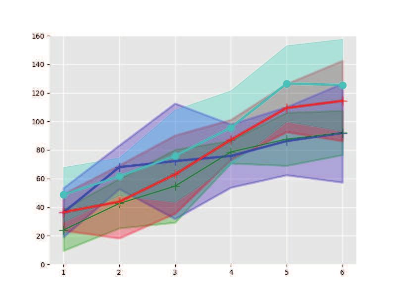
Published as a conference paper at ICLR 2019

The structure of the input convex neural network (ICNN) structure in Proposition 1 is motivated by the
structure in (Amos et al., 2017) but modified to be more suitable to control of dynamical systems. In
(Amos et al., 2017) it only requires W2:k to be non-negative while having no restrictions on weights
W1 and D2:k . Our construction achieves the exact representation by expanding the inputs to include
both u (∈ Rd ) and −u. Then any negative weights in W1 and D2:k in (Amos et al., 2017)’s ICNN
structure is set to zero and its negation (which is positive) is added as the weight for corresponding
−u. The reason for our construction is to allow the network to be “rolled out in time” when we are
dealing with dynamical systems and multiple networks need to be composed together.
An simple example that demonstrates how the proposed ICNN can be used to fit a convex function
comes form fitting the |u| function. This function is convex and both decreasing and increasing. Let
the activation function be ReLU(·) = max(·, 0). We can write |u| = −u + 2ReLU(u) (Amos et al.,
2017). However, in this representation, we need a negative weight, the −1 in front of u, and this
would be troublesome if we compose several networks together. In our proposed ICNN structure
with all positive weights and input negation duplicates, we can write |u| = v + 2ReLU(u), where
we impose a constraint v = −u. Such doubline on the number of input variables may potentially
make the network harder to train. Yet during control, having all of the weights positive maintains the
convexity between inputs and outputs even if multiple steps are considered which will be discussed in
Section 2.2. The constraint v = −u is linear and can be easily included in any convex optimization.
This proposition follows directly from composition of convex functions (Boyd & Vandenberghe,
2004). Although it allows for any increasing convex activation functions, in this paper we work with
the popular ReLU activation function. Two notable additions in ICNN compared with conventional
feedforward neural networks are: 1) Addition of the direct “passthrough” layers connecting inputs to
hidden layers and conventional feedforward layers connecting hidden layers for better representation
power. 2) the expanded inputs that include both u and −u. The proposed ICNN structure is shown
in Fig. 2(a). Note that such construction guarantees
                                                   that the network is convex and non-decreasing
                                            u
with respect to the expanded inputs û =        , while the output can achieve either decreasing or
                                           −u
non-decreasing functions over u.
Fundamentally, ICNN allows us to use neural networks in decision making processes by guaranteeing
the solution is unique and globally optimal. Since many complex input and output relationships can
be learned through deep neural networks, it is natural to consider using the learned network in an
optimization problem in the form of
                                              min f (u; W)                                            (1a)
                                                u
                                               s.t. u ∈ U ,                                           (1b)
where U is a convex feasible space. Then if f is an ICNN, optimizing over u is a convex problem,
which can be solved efficiently to global optimality. Note that we will always duplicate the variables
by introducing v = −u, but again this does not change the convexity of the problem. Of course,
since the weights of the network are restricted to be nonnegative, the performance of the network
(e.g., classification) may be worse. A common thread we observe in this paper is that trading off
classification performance with tractability can be preferable.

2.2   C LOSED - LOOP CONTROL AND RECURRENT NEURAL NETWORKS

In addition to the single-shot optimization problem in (1), we are interested in optimally controlling a
dynamical system. To model the temporal dependency of the system dynamics, we propose to use
recurrent neural networks (instead of feed-forward neural networks). Recurrent networks carry an
internal state of the system, which introduces coupling with previous inputs to the system. Fig. 2(b)
shows the proposed input convex recurrent neural networks (ICRNN) structure. This network maps
from input û to output y with memory unit z according to the following Eq. (2),
                                   zt = σ1 (Uût + Wzt−1 + D2 ût−1 ) ,                                (2)
                                   yt = σ2 (Vzt + D1 zt−1 + D3 ût ) ,                                 (3)

            u
where û =      , and D1 , D2 , D3 are added direct “passthrough” layers for augmenting representation
           −u
power. If we unroll the dynamics with respect to time, we have yt = f (û1 , û2 , ..., ût ; θ ) where θ =

                                                    4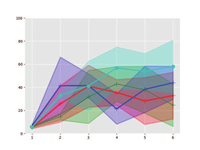
Published as a conference paper at ICLR 2019

[U, V, W, D1 , D2 , D3 ] are network parameters, and σ1 , σ2 denote the nonlinear activation functions.
The next proposition states a sufficient condition for the network to be input convex.
Proposition 2. The network shown in Fig. 2(b) is a convex function from inputs to output if all weights
U,V,W, D1 , D2 , D3 are non-negative, and all activation functions are convex and nondecreasing (e.g.
ReLU).
The proof of this proposition again follows directly from the composition rule of convex functions.
Similarly to the ICNN case, by expanding the inputs vector to include both u and −u and restricting
all weights to be non-negative, the resulted ICRNN structure is a convex and non-decreasing mapping
from inputs to output.
The proposed ICRNN structure can be leveraged to represent system dynamics for close-loop control.
Consider a physical system with discrete-time dynamics, at time step t, let’s define st as the system
states, ut as the control actions, and yt as the system output. For example, for the real-time control of
a building system, st includes the room temperature, humidity, etc; ut denotes the building appliance
scheduling, room temperature set-points, etc; and output yt is the building energy consumption. In
addition, there maybe exogenous variables that impact the output of the system, for example, outside
temperature will impact the energy consumption of the building. However, since the exogenous
variables are not impacted by any of the control actions we take, we suppress them in the formulation
below. The time evolution of a system is described by
                                                      yt = f (st , ut ) ,                                 (4a)
                                                    st+1 = g(st , ut )                                    (4b)
where (4b) describes the coupling between the current inputs to the future system states. Physical
systems described by (4) may have significant inertia in the sense that the outcome of any control
actions is delayed in time and there are significant couplings across time periods.
Since we use ICRNNs to represent both the system dynamics g(·) and the output f (·), the control
variable u expands as û. The optimal receding horizon control problem at time t can be written as,
                                                    t+T
                    minimize           C(x̂, y) =   ∑ J(x̂τ , yτ )                                        (5a)
                  ut ,ut+1 ,...,ut+T                τ=t
                     subject to yτ = f(x̂τ−nw , x̂τ−nw +1 , ..., x̂τ ), ∀τ ∈ [t,t + T ]                   (5b)
                                       sτ = g(x̂τ−nw , x̂τ−nw +1 , ..., x̂τ−1 , ûτ ) , ∀τ ∈ [t,t + T ]   (5c)

                                              sτ            u
                                       x̂τ =      , ûτ = τ , ∀τ ∈ [t,t + T ]                             (5d)
                                              ûτ           vτ
                                       vτ = −uτ , ∀τ ∈ [t,t + T ]                                         (5e)
                                       sτ ∈ S f easible , ∀τ ∈ [t,t + T ]                                  (5f)
                                       uτ ∈ U f easible , ∀τ ∈ [t,t + T ]                                 (5g)
where a new variable x̂ = [st , ût ] is introduced for notational simplicity, which called system inputs.
It is the collection of system states st and duplicated control actions ut and −ut , therefore ensuring
the mapping from ut to any future states and outputs remains convex. J(x̂τ , yτ ) is the control system
cost incurs at time τ, that is a function of both the system inputs x̂τ and output yτ . The functions
 f (·) and g(·) in Eq. (5b)-(5c) are parameterized as ICRNNs, which represent the system dynamics
from sequence of inputs (x̂τ−nw , x̂τ−nw +1 , ..., x̂τ ) to the system output yτ , and the dynamics from
control actions to system states, respectively. nw is the memory window length of the recurrent neural
network. The equations (5d) and (5e) duplicate the input variables u and enforce the consistency
condition between u and its negation v. Lastly, (5f) and (5g) are the constraints on feasible system
states and control actions respectively. Note that as a general formulation, we do not include the
duplication tricks on state variables, so the dynamics fitted by (5b) and (5c) are non-decreasing over
state space, which are not equivalent to those dynamics represented by linear systems. However,
since we are not restricting the control space, and we have explicitly included multiple previous
states in the system transition dynamics, so the non-decreasing constraint over state space should not
restrict the representation capacity by much. In Section.3 we theoretically prove the representability
of proposed networks.
Optimization problem in (5) is a convex optimization with respect to (w.r.t.) inputs u = [ut , ..., ut+T ],
provided the cost function J(x̂τ , yτ ) = J(sτ , ûτ , yτ ) is convex w.r.t. ûτ , and convex, nondecreasing

                                                             5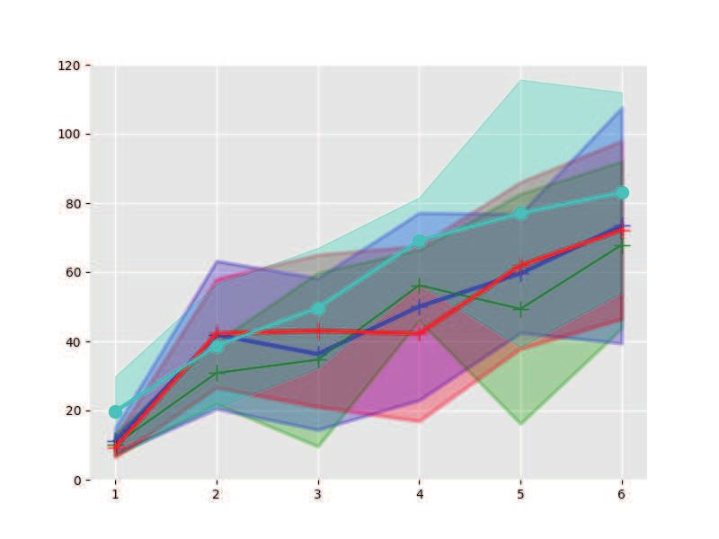
Published as a conference paper at ICLR 2019

w.r.t. sτ and yτ . A problem is convex if and only if both the objective function and constraints are
convex. In the above problem, J(sτ , ûτ , yτ ) is convex and nondecreasing w.r.t. sτ and yτ ; sτ and yτ
are parameterized as ICRNNs, i.e., (5a) and (5b), such that they are convex w.r.t. ûτ . Therefore
following the composition rule of convex functions, the objective function is convex w.r.t. inputs
u = [ut , ..., ut+T ]. Besides, all the equality constraints (5d) and (5e) are affine. Suppose both the
state feasibile set (5f) and action feasibile set (5g) are convex, the overall optimization is convex.
The convexity of the problem in (5) guarantees that it can be solved efficiently and optimally using
gradient descend method. Since both the objective function (5a) and the constraints (5b)-(5c) are
parameterized as neural networks, and their gradients can be calculated via back-propagation with
the modification where cost is propagated to the input rather than the weights of the network. For
implementation, the gradients can be convinently calculated via existing modules such as Tensorflow
viaback-propagation. Let u∗ = {ut∗ , ut+1 ∗ , ..., u∗ } be the optimal solution of the optimization
                                                    t+T
problem at time t. Then the first element of u∗ is implemented to the real-time system control, that is
ut∗ . The optimization problem is repeated at time t + 1, based on the updated state prediction using
ut∗ , yielding a model predictive control strategy.

3     E FFICIENCY AND REPRESENTATION POWER OF ICNN
Besides the computational traceability of the input convex networks, as an system identification
model, we are also interested its predictive accuracies and capacity. This section provides theoretical
analysis on the representation ability and efficiency of input convex neural networks.

3.1    R EPRESENTATION POWER OF INPUT CONVEX NEURAL NETWORK

Definition 1. Given a function f : Rd → R, we say that the function fˆ approximate f within ε if
| f (x) − fˆ(x)| ≤ ε for all x in the domain of f .
Theorem 1. [Representation power of ICNN] For any Lipschitz convex function over a compact
domain, there exists a neural network with nonnegative weights and ReLU activation functions that
approximates it within ε.
Lemma 1. Given a continuous Lipschitz convex function f : Rd → R with compact domain and
ε > 0, it can be approximated within ε by maximum of a finite number of affine functions. That is,
there exists fˆ(x) = maxi=1,...,N {µi T x + bi } such that | f (x) − fˆ(x)| ≤ ε for all x ∈ dom f .

Sketch of proof for Theorem 1. Supposing Lemma 1 is true, the proof of Theorem 1 boils down to
showing that neural network with nonnegative weights and ReLU activation functions can exactly
represent a maximum of affine functions. The proof is constructive. We first construct a neural
network with ReLU activation functions and both positive and negative weights, then we show that
the weights between different layers of the network can be restricted to be nonnegative by a simple
duplication trick. Specifically, since the weights in the input layer and passthrough layers in the ICNN
can be negative, we simply add a negation of each input variable (e.g. both x and −x are given as
inputs) to the network. These variables need satisfy a consistency constraint since one is the negation
of the other. Since this constraint is linear, it preserves the convexity of optimization problems. The
details of the proofs are given in the Appendix B.
This proof is similar in spirit to theorems in (Hanin, 2017; Arora et al., 2016). The key new result is a
simpler construction than the one used in (Hanin, 2017) and the restriction to nonnegative weights
between the layers.

Similar to Theorem 1, an analogous result about the representation power of ICRNN can be shown for
systems with convex dynamics. Given a dynamical system described by rolled out system dynamics
yt = f (x1 , . . . , xt ) is convex, then there exists a recurrent neural network with nonnegative weights
and ReLU activation functions that approximates it within ε. A broad range of systems can be
captured by this model. For example, the linear quadratic (Gaussian) regulator problem can be
described using a ICRNN if we identify y as the cost of the regulator (Skogestad & Postlethwaite,
2007; Boyd et al., 1994).1 An example of a nonlinear system is the control of electrochemical
    1 It’s important to note that y is usually used as the system output of a linear system, but in our context, we
are using it to refer to the quadratic cost with respect to the system states and the control input.

                                                        6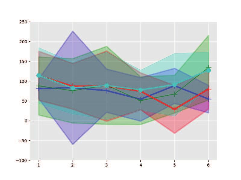
Published as a conference paper at ICLR 2019

batteries. It can be shown from first principles that the degradation of these types of batteries is
convex in their charge and discharge actions (Shi et al., 2018) and our framework offers a powerful
data-driven way to control batteries found in electric vehicles, cell phones, and power systems.

3.2   ICNN VS . CONVEX PIECEWISE LINEAR FITTING

In the proof of Theorem 1, we first approximate a convex function by a maximum of affine functions
then construct a neural network according to this maximum. Then a natural question is why learn
a neural network and not directly the affine functions in the maximum? This approach was taken
in (Magnani & Boyd, 2009), where a convex piecewise-linear function (max of affine functions) are
directly learned from data through a regression problem.
A key reason that we propose to use ICNN (or ICRNN) to fit a function rather than directly finding a
maximum of affine functions is that the former is a much more efficient parameterization than the
latter. As stated in Theorem 2, a maximum of K affine functions can be represented by an ICNN
with K layers, where each layer only requires a single ReLU activation function. However, given a
single layer ICNN with K ReLU activation functions, it may take a maximum of 2K affine functions
to represent it exactly. Therefore in practice, it would be much easier to train a good ICNN than
finding a good set of affine functions.
Theorem 2. [Efficiency of Representation]
      1. Let fICNN : Rd → R be an input convex neural network with K ReLU activation functions.
         Then Ω(2K ) functions are required to represent fICNN using a max of affine functions.
      2. Let fCPL : Rd → R be a max of K affine functions. Then O(K) activation functions are
         sufficient to represent fCPL exactly with an ICNN.

The proof of this theorem is given in Appendix C.

4     E XPERIMENTS
In this section, we verify the effectiveness of ICNN and ICRNN by presenting experimental re-
sults on two decision-making problems: continuous control benchmarks on MuJoco locomotion
tasks (Todorov et al., 2012) and energy management of reference large-scale commercial building
(Crawley et al., 2001), respectively. The proposed method can be used as a flexible building block in
decision making problems, where we use ICNN to represent system dynamics for MuJoco simulators,
and we use ICRNN in an end-to-end fashion to find the optimal control inputs. Both examples demon-
strate that proposed method: 1) discovers the connection between controllable variables and the
system dynamics or cost objectives; 2) is lightweight and sample-efficient; 3) achieves generalizable
and more stable control performances compared with previous model-based reinforcement learning
and simplified linear control approaches.

4.1   M U J O C O L OCOMOTION TASKS

Experimental Setup We consider four simulated robotic locomotion tasks: swimmer,
half-cheetah, hopper, ant implemented in MuJoCo under the OpenAI rllab frame-
work (Duan et al., 2016). We train and represent the locomotion state transition dynamics
st+1 =g(st ,ut )2 using a 2-layer ICNN with ReLU activations, which could be integrated into the
following finite-horizon control problem to find the optimal action sequence ut , ...,ut+T for fixed
looking ahead horizon T :
                                                  t+T
                                minimize        − ∑ r(sτ , uτ )                                             (6a)
                                 ut ,...,ut+T     τ=t
                                subject to sτ+1 = g(sτ , uτ ), ∀τ ∈ [t,t + T ]                              (6b)
                                           uτ ∈ U f easible , ∀τ ∈ [t,t + T ]                               (6c)
   2 Note that for notation convenience, in this example and the following building example, we use u to

represent the expanded control vector including its negation. For system state s ∈ Rd , if d > 1, convexity means
that each dimension of s is convex w.r.t. the function inputs.

                                                        7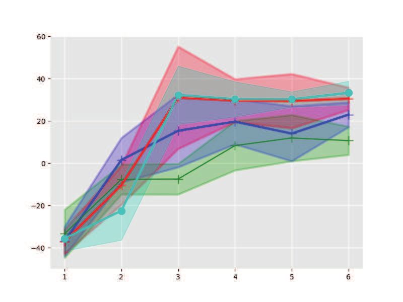
Published as a conference paper at ICLR 2019

where the objective (6a) is convex because r(sτ , uτ ) is a concave reward function related to system
states such as velocity and control actions (the detailed forms of r(sτ , uτ ) for different locomotion
tasks are listed in Appendix D). To achieve better model generalization on locomotion dynamics, we
also followed (Nagabandi et al., 2018), and applied DAGGER (Ross et al., 2011) to iteratively collect
labeled robotic rollouts and train the supervised dyamics model (6b) using on-policy locomotion
samples. See Appendix D for furthur simulation hyperparameters and experimental details. For each
aggregated iterations of collecting rollouts data and training ICNN model, we validate the controller
performance on standalone validation rollouts by optimally solving (6).

          Swimmer
                   Horizon=4                Horizon=10
                                                                + K=100         .
                                                                         Horizon=50
                                                                                    ICNN

Figure 3: Average rollout reward for random-shooting method vs ICNN on four MuJoCo tasks. The
horizontal axis indicates the aggregated iteration, and vertical axis indicates average reward. Plotted
curves are averaged over 3 random seeds, and the shaded region shows the standard deviation.

Baselines We compare our system modeling and continuous control method with state-of-the-art
model-based RL algorithm (Nagabandi et al., 2018), where the authors used a normal multi-layer
perceptrons (MLP) model to parameterize the system dynamics (6b). We refer to their method as
random-shooting algorithm, since they can not solve (6) to optimality, and they used pre-defined
number of random-shooting control sequences (denoted as K) to query the trained MLP and find
a best sequence as the rollout policy. Such a method is able to find good control policies in the
degree of 104 timesteps, which are much more sample-efficient than model-free RL methods (Duan
et al., 2016; Mnih et al., 2015). To make fair comparisons with baseline method, we keep the same
setup on the rollouts number and initial random action training. Our framework makes the neural
networks convex w.r.t input by adding passthrough links to the 2-layer model and keeping all the layer
weights nonnegative. We evaluate the performance of both algorithms on three randomly selected
fixed random seeds for four tasks. Similar to the fine tuning steps in (Nagabandi et al., 2018), control

                                                   8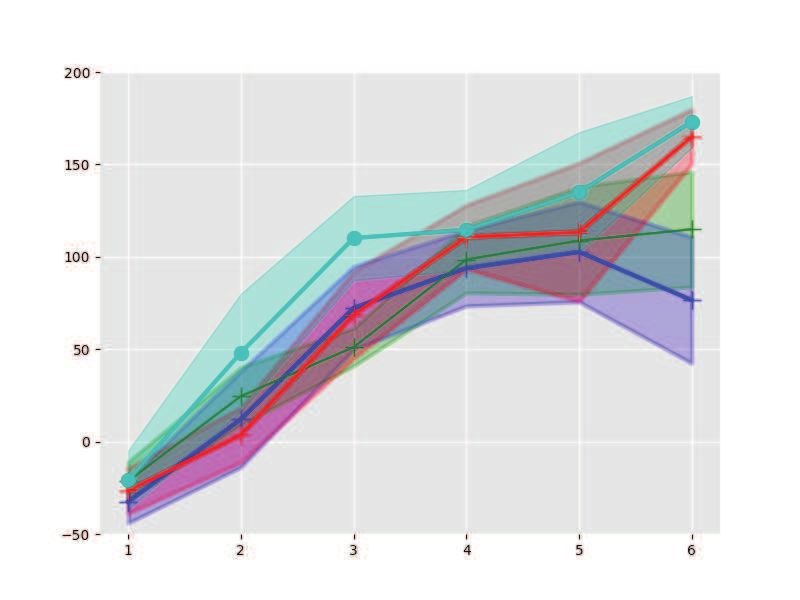
Published as a conference paper at ICLR 2019

policies found by ICNN can also be plugged in as initialized policies for subsequent model-free
reinforcement learning algorithms.
Continuous Control Performance During training, we found both ICNN and MLP are able to
predict robotic states quite accurately based on (6b). This provides a good system dynamics model
which is beneficial to solve control policies. The control performances are shown in Fig. 3, where we
compare the average reward of proposed method and random-shooting method with K = 100 over 10
validation rollouts during each aggregated iteration (see Fig. 8 in Appendix D.4 for random shooting
performance with varying K). The policy found by ICNN outperforms the random-shooting method
in all settings with varying horizon T for all of the four locomotion tasks.
Intuitively, ICNN should perform better when the action space is larger, since random-shooting
method can not search through the action space efficiently with a fixed K. This is illustrated in
the example of ant, where with more training samples aggregated and MLP model representing
more accurate dynamics, random-shooting gets stuck to find better control policies and there is little
improvement reflected in the control performance. Moreover, since we are skipping the expensive
process on calculating rewards of each random shooting trajectory and finding the best one, our
method only implements ICNN inference step based on (6) and is much faster than random shooting
methods in most settings, especially when K is large (see Table. 2 for wall-clock time in Appendix
D.3). For instance, in the case of Swimmer, our proposed method only uses 15 of time compared
to (Nagabandi et al., 2018). This also indicates that our method is even much more sample-efficient
than off-the-shelf model-free RL methods, where we use two orders of magnitude less training data to
reach similar validation rewards (Duan et al., 2016; Mnih et al., 2015) (see Fig. 9 in Appendix D.4).

4.2   B UILDING E NERGY M ANAGEMENT

Experimental Setup We now move on to optimally control a dynamical system with significant
inertia. We consider the real-time control problem of building’s HVAC (heating, ventilation, and air
conditioning) system to reduce its energy consumption. Building energy management remains to be
a hard problem in control area. The exact system dynamics are unknown and hard to model due to
the complex heating transfer dynamics, time-varying environments and the scale of the system in
terms of states and actions (Kouro et al., 2009). At time t, we assume the building’s running profile
xt := [st , ut ] is available, where st denotes building system states, including outside temperature, room
temperature measurements, zone occupancies and etc. ut denotes a collection of control actions such
as room temperature set points and appliance schedule. Output is the electricity consumption Pt .
This is a model predictive control problem in the sense that we want to find the best control inputs
that minimize the overall energy consumption of building by looking ahead several time steps. To
achieve this goal, we firstly learn an ICRNN model f (·) of the building dynamics, which is trained to
minimize the error between Pt and f (xt−nw , ..., xt ), while nw denotes the memory window of recurrent
neural networks. Then we solve:

                                        t+T
                         minimize
                         ut ,...,ut+T
                                        ∑ f (xτ−nw , ..., xτ )                                        (7a)
                                        τ=t
                        subject to sτ = g(xτ−nw , ..., xτ−1 , uτ ), ∀τ ∈ [t,t + T ]                   (7b)
                                   uτ ≤ uτ ≤ uτ , ∀τ ∈ [t,t + T ]                                     (7c)
                                   sτ ≤ sτ ≤ sτ , ∀τ ∈ [t,t + T ]                                     (7d)

where the objective (7a) is minimizing the total energy consumption in future T steps (T is the
model predictive control horizon), and (7b) is used for modeling building states, in which g(·) are
parameterized as ICRNNs. Note that the formulation (7) is also flexible with different loss functions.
For instance, in practice, we could reuse trained dynamics model (7b), and integrate electricity prices
into the overall objective so that we could directly learn real-time actions to minimize electricity
bills (please refer to Appendix E for more results). The constraints on control actions ut and
system states st are given in (7c) and (7d). For instance, the temperature set points as well as real
measurements should not exceed user-defined comfort regions.

                                                       9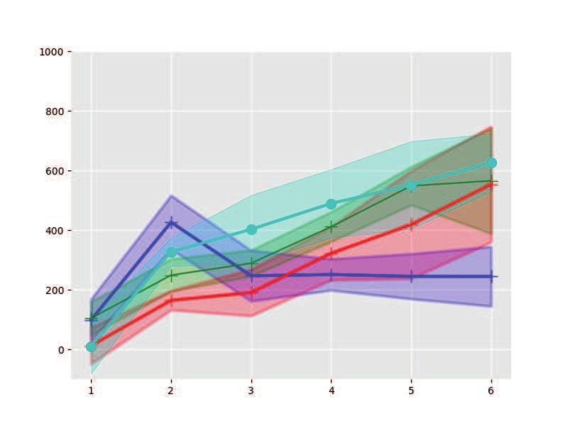
Published as a conference paper at ICLR 2019

                                     Ground Truth     ICRNN         Normal RNN            RC Model                      (c)                        Basement
                                                                                                                                     24
    (a)                                      Dynamics Fitting              (b)            Control Performance                        23

                                                                                                                       Temperature [C]
                                 8                                                  8
                         8× 10                                             8 × 10                                                    22
                                                                                                                                     21
                         7                                                 7
Energy Consumption [J]
                                                                                                                                     20
                                                                                                                                     19
                         6                                                 6
                                                                                                                                     18
                                                                                                                                              Mon Tue Wed Thu     Fri
                         5                                                 5                                                                       Top Middle
                                                                                                                                         24
                         4                                                 4

                                                                                                                          Temperature [C]
                                                                                                                                         23
                                                                                                                                         22
                         3                                                 3
                                                                                                                                         21

                         2                                                 2                                                             20
                                                                                                                                         19
                                 Mon        Tue     Wed       Thu    Fri            Mon     Tue      Wed   Thu   Fri                     18
                                                                                                                                              Mon Tue   Wed Thu   Fri

Figure 4: Results for constrained optimization of building energy management. (a) ICRNN is able to
model the building dynamics as accurately as conventional RNN; (b) Compared to conventional RNN
model, ICRNN finds control actions which lead to 11.52% more of energy savings, and (c) ICRNN
provides stable control actions while decisions generated by conventional RNN vary dramatically.

To test the performance of the proposed method, we set up a 12-story large office building, which is a
reference EnergyPlus commercial building model from US Department of Energy (DoE) 3 , with a
total floor area of 498, 584 square feet which is divided into 16 separate zones. By using the whole
year’s weather profile, we simulate the building running through the year and record (xt , Pt ) with
a resolution of 10 minutes. We use 10 months’ data to train the ICRNN and subsequent 2 months’
data for testing. We use 39 building system state variables st (uncontrollable), along with 16 control
variables ut . Output is a single value of building energy consumption at each time step. We set the
model predictive control horizon T = 36 (six hours). We employ an ICRNN with recurrent layer of
dimension 200 to fit the building input-output dynamics f (·). The model is trained to minimize the
MSE between its predictions and the actual building energy consumption using stochastic gradient
descent. We use the same network structure and training scheme to fit state transition dynamics g(·).
Baseline We set the model-based forecasting and optimization benchmark using an linear resistor-
circuit (RC) circuit model to represent the heat transfer in building systems, and solve for the optimal
control actions via MPC (Ma et al., 2012). At each step, MPC algorithm takes into account the
forecasted states of the building based on the fitted RC model and implements the current step control
actions. We also compare the performance of ICRNN against the conventionally trained RNN in
terms of building dynamics fitting performance and control performance. To solve the MPC problem
with conventional RNN models, we also use gradient-based method with respect to controls. However,
since conventional RNN models are generally not convex from input to output, there is no guarantee
to reach a global optimum (or even a local one).
Results In terms of the fitting performance, ICRNN provides a competitive result compared to
conventional RNN model. The overall test root mean square error (RMSE) is 0.054 for ICRNN
and 0.051 for conventional RNN, both of which are much smaller than the error made by RC
model (0.240). Fig. 4(a) shows the fitting performance on 5 working days in test data. This illustrates
the good performance of ICRNN in modeling building HVAC system dynamics. Then by using the
learned ICRNN model of building dynamics, we obtain the suggested room control actions ut∗ by
solving the optimal building control problem (7). As shown in Fig. 4(b), with the same constraints on
building temperature interval of [19◦C, 24◦C], the building energy consumption is reduced by 23.25%
after implementing the new temperature set points calculated by ICRNN. On the contrary, since there
is no guarantee for finding optimal control actions by optimizing over conventional RNN’s input,
the control solutions given by conventional RNN could only reduce 11.73% of electricity. Solutions
given by RC model only saves 4.07% of electricity. More importantly, in Fig. 4(c) we demonstrate
the control actions outputted by our method against MPC with conventional RNN in two randomly
selected building zones, the building basement and top floor central area. It shows that our proposed

   3 Energyplus is an open-source whole-building energy modeling software, which is developed by US DoE for
standard building energy simulation

                                                                                          10
Published as a conference paper at ICLR 2019
approach is able to find a group of stable control actions for the building system control. While in the
conventional RNN case, it generates control set points which have undesirable, drastic variations.
5 S UMMARY AND D ISCUSSION
In this work we proposed a novel optimal control framework that uses deep neural networks engi-
neered to be convex from the input to the output. This framework bridges machine learning and
control by representing system dynamics using input convex (recurrent) neural networks. We show
that many interesting data-driven control problems can be cast as convex optimization problems using
the proposed network architecture. Experiments on both benchmark MuJoCo locomotion tasks and
building energy management demonstrate our methodology’s potential in a variety of control and
optimization problems.
R EFERENCES
Brandon Amos, Lei Xu, and J Zico Kolter. Input convex neural networks. In International Conference
on Machine Learning, pp. 146–155, 2017.
Raman Arora, Amitabh Basu, Poorya Mianjy, and Anirbit Mukherjee. Understanding deep neural
networks with rectified linear units. arXiv preprint arXiv:1611.01491, 2016.
Stephen Boyd and Lieven Vandenberghe. Convex optimization. Cambridge university press, 2004.
Stephen Boyd, Laurent El Ghaoui, Eric Feron, and Venkataramanan Balakrishnan. Linear matrix
inequalities in system and control theory, volume 15. Siam, 1994.
Chia-Chin Cheng, S Pouffary, N Svenningsen, and John M Callaway. The kyoto protocol, the clean
development mechanism and the building and construction sector: A report for the unep sustainable
buildings and construction initiative, 2008.
Morris G Cox. An algorithm for approximating convex functions by means by first degree splines.
The Computer Journal, 14(3):272–275, 1971.
Drury B Crawley, Linda K Lawrie, Frederick C Winkelmann, Walter F Buhl, Y Joe Huang, Curtis O
Pedersen, Richard K Strand, Richard J Liesen, Daniel E Fisher, Michael J Witte, et al. Energyplus:
creating a new-generation building energy simulation program. Energy and buildings, 33(4):
319–331, 2001.
Marc Peter Deisenroth, Carl Edward Rasmussen, and Dieter Fox. Learning to control a low-cost
manipulator using data-efficient reinforcement learning. 2011.
Yan Duan, Xi Chen, Rein Houthooft, John Schulman, and Pieter Abbeel. Benchmarking deep
reinforcement learning for continuous control. In International Conference on Machine Learning,
pp. 1329–1338, 2016.
Momčilo M Gavrilović. Optimal approximation of convex curves by functions which are piecewise
linear. Journal of Mathematical Analysis and Applications, 52(2):260–282, 1975.
Boris Hanin. Universal function approximation by deep neural nets with bounded width and relu
activations. arXiv preprint arXiv:1708.02691, 2017.
Kaiming He, Xiangyu Zhang, Shaoqing Ren, and Jian Sun. Deep residual learning for image
recognition. In Proceedings of the IEEE conference on computer vision and pattern recognition,
pp. 770–778, 2016.
Kenji Kawaguchi. Deep learning without poor local minima. In Advances in Neural Information
Processing Systems, pp. 586–594, 2016.
Samir Kouro, Patricio Cortés, René Vargas, Ulrich Ammann, and José Rodríguez. Model predictive
control—a simple and powerful method to control power converters. IEEE Transactions on
industrial electronics, 56(6):1826–1838, 2009.
11Published as a conference paper at ICLR 2019
Sergey Levine and Vladlen Koltun. Learning complex neural network policies with trajectory
optimization. In International Conference on Machine Learning, pp. 829–837, 2014.
Sergey Levine, Chelsea Finn, Trevor Darrell, and Pieter Abbeel. End-to-end training of deep
visuomotor policies. The Journal of Machine Learning Research, 17(1):1334–1373, 2016.
Lennart Ljung. System identification. In Signal analysis and prediction, pp. 163–173. Springer, 1998.
Yudong Ma, Anthony Kelman, Allan Daly, and Francesco Borrelli. Predictive control for energy
efficient buildings with thermal storage: Modeling, stimulation, and experiments. IEEE Control
Systems, 32(1):44–64, 2012.
Alessandro Magnani and Stephen P Boyd. Convex piecewise-linear fitting. Optimization and
Engineering, 10(1):1–17, 2009.
David Meger, Juan Camilo Gamboa Higuera, Anqi Xu, Philippe Giguere, and Gregory Dudek.
Learning legged swimming gaits from experience. In Robotics and Automation (ICRA), 2015
IEEE International Conference on, pp. 2332–2338. IEEE, 2015.
Volodymyr Mnih, Koray Kavukcuoglu, David Silver, Alex Graves, Ioannis Antonoglou, Daan
Wierstra, and Martin Riedmiller. Playing atari with deep reinforcement learning. arXiv preprint
arXiv:1312.5602, 2013.
Volodymyr Mnih, Koray Kavukcuoglu, David Silver, Andrei A Rusu, Joel Veness, Marc G Bellemare,
Alex Graves, Martin Riedmiller, Andreas K Fidjeland, Georg Ostrovski, et al. Human-level control
through deep reinforcement learning. Nature, 518(7540):529, 2015.
Anusha Nagabandi, Gregory Kahn, Ronald S Fearing, and Sergey Levine. Neural network dynam-
ics for model-based deep reinforcement learning with model-free fine-tuning. In 2018 IEEE
International Conference on Robotics and Automation (ICRA), pp. 7559–7566. IEEE, 2018.
Daniel O’Neill, Marco Levorato, Andrea Goldsmith, and Urbashi Mitra. Residential demand response
using reinforcement learning. In Smart Grid Communications (SmartGridComm), 2010 First IEEE
International Conference on, pp. 409–414. IEEE, 2010.
Stéphane Ross, Geoffrey Gordon, and Drew Bagnell. A reduction of imitation learning and structured
prediction to no-regret online learning. In Proceedings of the fourteenth international conference
on artificial intelligence and statistics, pp. 627–635, 2011.
HL Royden and PM Fitzpatrick. Real analysis. 4th, 2010.
John Schulman, Sergey Levine, Pieter Abbeel, Michael Jordan, and Philipp Moritz. Trust region
policy optimization. In International Conference on Machine Learning, pp. 1889–1897, 2015.
Pervez Hameed Shaikh, Nursyarizal Bin Mohd Nor, Perumal Nallagownden, Irraivan Elamvazuthi,
and Taib Ibrahim. A review on optimized control systems for building energy and comfort
management of smart sustainable buildings. Renewable and Sustainable Energy Reviews, 34:
409–429, 2014.
Y. Shi, B. Xu, Y. Tan, D. Kirschen, and B. Zhang. Optimal battery control under cycle aging
mechanisms in pay for performance settings. IEEE Transactions on Automatic Control, pp. 1–1,
2018. ISSN 0018-9286. doi: 10.1109/TAC.2018.2867507.
Sigurd Skogestad and Ian Postlethwaite. Multivariable feedback control: analysis and design,
volume 2. Wiley New York, 2007.
Nagender Kumar Suryadevara, Subhas Chandra Mukhopadhyay, Sean Dieter Tebje Kelly, and
Satinder Pal Singh Gill. Wsn-based smart sensors and actuator for power management in intelligent
buildings. IEEE/ASME transactions on mechatronics, 20(2):564–571, 2015.
Emanuel Todorov, Tom Erez, and Yuval Tassa. Mujoco: A physics engine for model-based control.
In Intelligent Robots and Systems (IROS), 2012 IEEE/RSJ International Conference on, pp. 5026–
5033. IEEE, 2012.
12Published as a conference paper at ICLR 2019
Ashish Vaswani, Noam Shazeer, Niki Parmar, Jakob Uszkoreit, Llion Jones, Aidan N Gomez, Łukasz
Kaiser, and Illia Polosukhin. Attention is all you need. In Advances in Neural Information
Processing Systems, pp. 6000–6010, 2017.
Shuning Wang. General constructive representations for continuous piecewise-linear functions. IEEE
Transactions on Circuits and Systems I: Regular Papers, 51(9):1889–1896, 2004.
T. Wei, Y. Wang, and Q. Zhu. Deep reinforcement learning for building hvac control. In The Design
and Automation Conference, 2017.
W. Wolf. Cyber-physical systems. Computer, 42:88–89, 2009.
Zhaohui Zhang, Ruilong Deng, Tao Yuan, and S Joe Qin. Distributed optimization of multi-building
energy systems with spatially and temporally coupled constraints. In American Control Conference
(ACC), 2017, pp. 2913–2918. IEEE, 2017.
13Published as a conference paper at ICLR 2019
A PPENDIX
A. T OY E XAMPLE
Consider a synthetic example which contains two circles of noisy input data u ∈ R2 , along with
discrete data label y ∈ {0, 1} which is based on input coming from inner loop (y = 0) or outer
loop (y = 1). Suppose a decision maker is interested in finding the u that maximizes the probability
of y being 0. This optimization problem can be solved by firstly learning a neural network classifier
from u to y, and then to find the u point which minimizes the output of the neural network. More
specifically, let fNN be a conventional neural network and fICNN be an ICNN. Then the objective
becomes minimizing fNN (u) or fICNN (u).
Figure 5 shows the decision boundaries for fNN and fICNN , respectively. These networks are composed
of 2 hidden layers, with 200 neurons in each layer, and are trained using the same random seed, same
number of samples (100) until loss convergence. The decision boundaries of a conventional network
have many “zigzags”, which makes solving (1) challenging, especially if u is constrained. In contrast,
the ICNN has convex level sets (by construction) as decision boundaries, which leads to a convex
optimization problem.
u2
u2
u1 u1
Figure 5: Toy example on classifying circle data with label 0 (blue cross) and label 1 (red cross)
along with conventional neural networks (left) and ICNN (right) decision contour lines. A decision
maker is interested in finding a u that has the highest probability of being labeled 0.
A PPENDIX B. P ROOF OF T HEOREM 1
Proof. Lemma 1 follows from well established facts in function analysis stating that piecewise
linear functions are dense in the space of all continuous functions over compact sets (Royden
& Fitzpatrick, 2010) and convex piecewise linear functions are dense in the space of all convex
continuous functions (Cox, 1971; Gavrilović, 1975). Using the fact that convex piecewise linear
functions can be represented as a maximum of affine functions (Magnani & Boyd, 2009; Wang, 2004)
gives the desired result in the lemma.
Lemma 1 shows that all continuous Lipschitz convex functions f (x) : Rd → R over convex compact
sets can be approximated using maximum of affine functions. Then it suffices to show that an ICNN
can exactly represent a maximum of affine functions. To do this, we first construct a neural network
with ReLU activation function with both positive and negative weights that can represent a maximum
of affine functions. Then we show how to restrict all weights to be nonnegative.
As a starting example, consider a maximum of two affine functions
fCPL (x) = max{aT1 x + b1 , aT2 x + b2 }. (8)
To obtain the exact same function using a neural network, we first rewrite it as
fCPL (x) = (aT2 x + b2 ) + max (a1 − a2 )T x + (b1 − b2 ), 0 .
(9)
Now define a two-layer neural network with layers z1 and z2 as shown in Fig. 6:
z1 = σ (a1 − a2 )T x + (b1 − b2 ) ,
(10a)
z2 = z1 + aT2 x + b2 (10b)
14Published as a conference paper at ICLR 2019
where σ is the ReLU activation function and the second layer is linear. By construction, this neural
network is the same function as fCPL given in (8).
D2
x W1 z1 W2 z2
Figure 6: A simple two-layer neural networks. In alignment with (10), W1 denotes the first-layer
weights a1 − a2 and bias b1 − b2 , and W2 denotes the linear second layer. Direct layer is denoted as
D2 for weights a2 and bias b2 .
The above argument extends directly to a maximum of K linear functions. Suppose
fCPL (x) = max{aT1 x + b1 , ..., aTK x + bK } (11)
Again the trick is to rewrite fCPL (x) as a nested maximum of affine functions. For notational
convenience, let Li = aTi x + bi , Li0 = Li − Li+1 . Then
fCPL = max{L1 , L2 , ..., LK }
= max{max{L1 , L2 , ..., LK−1 }, LK }
= LK + σ (max{L1 , L2 , ..., LK−1 } − LK )
= LK + σ (max{max{L1 , L2 , ..., LK−2 }, LK−1 } − LK , 0)
= LK + σ (LK−1 − LK + σ (max{L1 , L2 , ..., LK−2 } − LK−1 , 0) , 0)
= ...
0 0
+ σ ...σ L20 + σ (L1 − L2 , 0) , 0 , ..., 0 , 0 , 0 .
= LK + σ LK−1 + σ LK−2
The last equation describes a K layer neural network, where the layers are:
z1 = σ (L1 − L2 , 0) = σ (a1 − a2 )T x + (b1 − b2 ) ,
z2 = σ L20 + z1 , 0 = σ z1 + (a2 − a3 )T x + (b2 − b3 ) ,
......
zi = σ Li0 + zi−1 , 0 = σ zi−1 + (ai − ai+1 )T x + (bi − bi+1 ) ,
......
zK = zK−1 + LK = hK (zK−1 + LK ) = zK−1 + aTK x + bK .
Each layer of of this neural network uses only a single activation function.
Although the above neural network exactly represent a maximum of linear functions, it is not convex
since the coefficients between layers could be negative. In particular, each layer involves an inner
product of the form (ai − ai+1 )T x and the coefficients are not necessarily nonnegative. To overcome
this, we simply expand the input to include x and −x. Namely, define a new input x̂ ∈ R2d as
x
x̂ = . (12)
−x
15Published as a conference paper at ICLR 2019
Then any inner product of the form hT x can be written as
d
hT x = ∑ hi xi
j=1
= ∑ hi xi + ∑ hi xi
i:hi ≥0 i:hiPublished as a conference paper at ICLR 2019
Environment Swimmer Half-Cheetah Hopper Ant
Reward Function vel − 0.5|| u ||2
st+1 vel − 0.05|| u ||2
st+1 vel + 1 −
st+1 vel + 0.5 −
st+1
50 2 1 2
u 2 u 2
0.005|| 200 ||2 0.005|| 150 ||2
Rollout Horizon 333 1000 200 1000
Rollout Numbers 25 10 30 400
Training Epochs 60 60 40 60
Table 1: Environment and training details for four MuJoCo locomotion tasks.
A PPENDIX D. E XPERIMENTAL D ETAILS ON M U J O C O TASKS
D.1 DATA C OLLECTION
Rollout Samples To train the neural network dynamics model (both ICNN and MLP), we first
collect initial rollout data using fully random action sequences ut ∼ Uniform[-1, 1] with a random
chosen initial state. During the data collection process in aggregated iterations, to improve model
generalization and explore larger state spaces, we add Gaussian noise to the optimal control policies
ut = ut + N (0, 0.001).
Neural Networks Training We represent the MuJoCo dynamics with a 2-hidden-layer neural net-
works with hidden sizes 512 − 512. The passthrough links of ICNN are of same size of corresponding
added layers. We train both models using Adam optimizer with a learning rate 0.001 and a mini-batch
size of 512. Due to the different complexity of MuJoCo tasks, we vary training epochs and summarize
the training details in Table. 1.
D.2 E NVIRONMENT D ETAILS
In all of the MuJoCo locomotion tasks, s includes state variables such as robot positions, velocity
along each axis; u includes action efforts for the agent. We use standard reward functions r(st , ut ) for
moving tasks, which could be also promptly calculated in (6a) as the control objective. For the ease
of neural network training and action sampling, we normalize all the action and states in the range of
[−1, 1]. We use DAGGER (Ross et al., 2011) for 6 aggregated iterations for all cases, and during
aggregated iteration, we use a split of 10% random rollouts collected as described in 5, and other 90%
coming from past iterations’ control policies (on-policy rollouts). Note that we use 10 random control
sequences in our method to initialize the policy finding approach and avoid the long computation time
for taking gradients on finding optimal ut . Other environment parameters are described in Table. 1.
D.3 WALL -C LOCK T IME
In Table.2, we show the average run time for the total of 6 aggregation iterations over 3 runs. Finding
control policies via ICNN is using less or equal training time compared to random-shooting method
with K = 100, while achieving better task rewards than K = 1000 for different control horizons. All
the experiments are running on a computer with 8 cores Intel I7 6700 CPU. Note that we do not
use GPU for accelerating ICNN optimization step (6), which could furthur improve our method’s
efficiency.
D.4 D ETAILS OF S IMULATION R ESULTS
MuJoCo Dynamics Modeling In Fig. 7, we compare the ICNN and normal MLP fitting perfor-
mance of the MuJoCo dynamics modeling (6b), which illustrates that both MLP and ICNN are able
to find a data-driven dynamics model for ant MuJoCo agent, which is of the most complex dynamics
we considered for locomotion tasks. The multi-step prediction errors of ICNN is comparable to
normal MLP used in (Nagabandi et al., 2018) for different length of rollout steps.
17Published as a conference paper at ICLR 2019
Swimmer
K = 100 K = 300 K = 1000 ICNN
H =4 18.36 18.48 40.20 16.41
H = 10 21.74 25.41 71.49 18.71
H = 50 40.01 70.31 169.49 36.24
Half-Cheetah
K = 100 K = 300 K = 1000 ICNN
H =4 34.40 47.72 88.49 34.93
H = 10 48.86 74.60 181.34 36.39
H = 50 113.58 275.61 816.32 83.66
Hopper
K = 100 K = 300 K = 1000 ICNN
H =4 5.48 6.30 7.76 5.61
H = 10 5.97 7.89 9.34 5.14
H = 50 10.89 14.77 38.02 9.16
Ant
K = 100 K = 300 K = 1000 ICNN
H =4 399.39 415.51 433.35 349.13
H = 10 480.60 481.34 511.93 459.63
H = 50 979.73 1024.5 1075.52 929.5
Table 2: Average wall clock time (in minutes) for random-shooting model-based reinforcement
learning method and ICNN.
+ MLP . ICNN
1000
100
Ant Dynamics Prediction Error
10
1
0.1
0.01
0.001 1 5 10 50 100
Rollout Steps
Figure 7: Multistep prediction errors by ICNN and MLP. X-Axis and Y-Axis are of log scale.
More Simulation Results In Fig. 8, we compare our control method with random-shooting approach
with varying settings on shooting number K, which shows that our approach is more efficient in
finding control policies.
In Fig. 9, we compare our control method with the rllab implementation of trust region policy
optimization (TRPO) (Schulman et al., 2015), an end-to-end deep reinforcement learning approach
for mujoco locomotion tasks. More specifically, we compare the algorithms’ performances with
relatively few available rollout samples. While our approach quickly learns the dynamics and
then find control actions via optimization steps, TRPO is hard to learn the actions directly with
few provided rollouts. Similarly to the model-based and model-free (Mb-Mf) approach described
18You can also read