On the interpretation of ice-shelf flexure measurements
←
→
Page content transcription
If your browser does not render page correctly, please read the page content below
Journal of Glaciology (2017), 63(241) 783–791                                                                               doi: 10.1017/jog.2017.44
       © The Author(s) 2017. This is an Open Access article, distributed under the terms of the Creative Commons Attribution licence (http://creativecommons.
       org/licenses/by/4.0/), which permits unrestricted re-use, distribution, and reproduction in any medium, provided the original work is properly cited.

                     On the interpretation of ice-shelf flexure measurements
                    SEBASTIAN H. R. ROSIER,1* OLIVER J. MARSH,2 WOLFGANG RACK,2
                   G. HILMAR GUDMUNDSSON,1 CHRISTIAN T. WILD,2 MICHELLE RYAN2
                                                                1
                                                             British Antarctic Survey, Cambridge, UK
                                         2
                                             Gateway Antarctica, University of Canterbury, Christchurch, New Zealand
                                                  *Correspondence: Sebastian Rosier

                     ABSTRACT. Tidal flexure in ice shelf grounding zones has been used extensively in the past to determine
                     grounding line position and ice properties. Although the rheology of ice is viscoelastic at tidal loading
                     frequencies, most modelling studies have assumed some form of linear elastic beam approximation to
                     match observed flexure profiles. Here we use density, radar and DInSAR measurements in combination
                     with full-Stokes viscoelastic modelling to investigate a range of additional controls on the flexure of the
                     Southern McMurdo Ice Shelf. We find that inclusion of observed basal crevasses and density dependent
                     ice stiffness can greatly alter the flexure profile and yet fitting a simple elastic beam model to that profile
                     will still produce an excellent fit. Estimates of the effective Young’s modulus derived by fitting flexure
                     profiles are shown to vary by over 200% depending on whether these factors are included, even
                     when the local thickness is well constrained. Conversely, estimates of the grounding line position are
                     relatively insensitive to these considerations for the case of a steep bed slope in our study region. By
                     fitting tidal amplitudes only, and ignoring phase information, elastic beam theory can provide a good
                     fit to observations in a wide variety of situations. This should, however, not be taken as an indication
                     that the underlying rheological assumptions are correct.
                     KEYWORDS: ice/ocean interactions, ice rheology, ice-sheet modelling, ice shelves

       1. INTRODUCTION                                                                          1983; Rist and others, 1996; Petrenko and Whitworth,
       The grounding zone, where ice transitions from grounded to                               2002). Alternatively, assumptions about ice rheology have
       freely floating, is a narrow but crucial portion of marine ice                           been made in order to invert tidal flexure curves for ice thick-
       sheets. Ocean tides beneath the ice shelf lead to ice                                    ness in the grounding zone (Marsh and others, 2014). Finally,
       flow modulation far upstream of the grounding line                                       (D)InSAR (Differential Interferometric Synthetic Aperture
       (Anandakrishnan and others, 2003; Bindschadler and                                       Radar) has become a common tool to determine GL position,
       others, 2003; Gudmundsson, 2006) and the flexure of ice                                  either through fitting an elastic beam model to tidal fringes
       in this region can be used as an indicator of grounding line                             (Rignot, 1998a, b; Sykes and others, 2009) or by positioning
       (GL) position (Goldstein and others, 1993; Rignot, 1998a, b;                             it at the location in a differential interferogram where vertical
       Sykes and others, 2009; Rignot and others, 2011) and migra-                              motion is detected above noise for the first time (Rignot and
       tion (Brunt and others, 2011). Ice-sheet mass balance is often                           others, 2011). Here, we question the validity of some of the
       estimated as the difference between net accumulation                                     approaches listed above.
       upstream of the GL and mass flux across it but this calculation                              Ice stiffness, typically described by the Young’s modulus
       is sensitive to uncertainty in the GL position and ice thickness                         (E), is important for the transmission of elastic stresses
       at the GL (Shepherd and others, 2012).                                                   through ice and is a crucial parameter when considering its
           Studies of ice-shelf tidal flexure have been used frequently                         fracture or damage. Elastic stresses play a key role in the
       to seek insights into ice rheology and determine GL position                             propagation of (relatively) high frequency tidal motion
       based on a given flexure profile. Ice in the grounding zone                              through ice (Gudmundsson, 2007, 2011; Walker and
       bends to accommodate the vertical motion of the adjoining                                others, 2012; Thompson and others, 2014; Rosier and
       ice shelf resulting from ocean tides. In the past this has typic-                        others, 2015; Rosier and Gudmundsson, 2016) and any
       ally been modelled as some form of elastic beam/plate equa-                              weakening in shear margins due to crevasses could partly
       tion (Holdsworth, 1969, 1977; Lingle and others, 1981;                                   explain the large distances upstream that these signals are
       Smith, 1991; Vaughan, 1995; Schmeltz and others, 2002;                                   observed (Thompson and others, 2014). Ice stiffness is also
       Sykes and others, 2009; Sayag and Worster, 2011, 2013;                                   an important parameter for the fracture toughness of ice.
       Walker and others, 2013; Marsh and others, 2014; Hulbe                                   Estimates of this parameter obtained by fitting a beam
       and others, 2016). Some of these studies seek to determine                               model to flexure profiles have recently been used to model
       the elastic (Young’s) modulus of glacial ice in situ by match-                           strand crack formation in the grounding zone (Hulbe and
       ing beam theory to observed flexure profiles (e.g. Lingle and                            others, 2016).
       others, 1981; Stephenson, 1984; Kobarg, 1988; Smith, 1991;                                   Direct comparisons cannot be made between laboratory
       Vaughan, 1995; Schmeltz and others, 2002; Sykes and                                      measurements of ice elasticity and those obtained from
       others, 2009; Hulbe and others, 2016) as an alternative to                               fitting models to ice-shelf flexure profiles, as ice is not
       seismic or mechanical laboratory experiments (e.g. Jellinek                              purely elastic over tidal timescales (Schmeltz and others,
       and Brill, 1956; Dantl, 1968; Roethlisberger, 1972; Hutter,                              2002; Reeh and others, 2003; Wild and others, 2017). The

Downloaded from https://www.cambridge.org/core. 23 Jan 2021 at 20:00:37, subject to the Cambridge Core terms of use.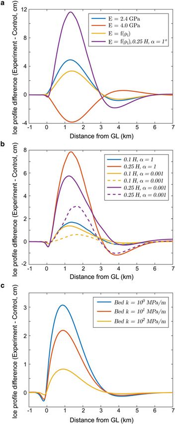
784                                                                                   Rosier and others: On the interpretation of ice-shelf flexure measurements

           true elastic modulus and the ‘effective’ modulus observed in                             change the interpretation of ice rheology. A quantitive ana-
           the field are material properties of two separate rheological                            lysis of the effects of crevassing and vertical density variation
           models. In reality, deformation of ice crystal fabric and                                on the tidal flexure of ice in the grounding zone are investi-
           change in bulk structure due to accumulated strain leads to                              gated for the first time. We compare results between a
           a nonlinear variation in strain rate and an overall softening                            linear elastic beam model and a 2-D full-Stokes viscoelastic
           of the ice over time. This cannot be observed in the instant-                            finite element model that has been used in the past to explore
           aneous elastic response. As well as providing a misleading                               ice/tide processes (Gudmundsson, 2011; Rosier and others,
           Young’s modulus, a purely elastic model of ice at tidal time-                            2014, 2015; Rosier and Gudmundsson, 2016). The model
           scales can only transmit stresses instantaneously with no                                domain is based on a comprehensive recent survey of the
           phase lag. In contrast, while still not matching all time-depend-                        grounding zone of White Island on the Southern McMurdo
           ent changes in ice fabric, a realistic viscoelastic rheology                             Ice Shelf, including ice thickness measurements and loca-
           incorporates the delayed viscous signal, which changes ice                               tions of probable basal crevasses obtained by radar (Fig. 1).
           stream response to tidal forcing and leads to long-period                                This extensive dataset provides a unique opportunity to
           modulation in velocity (Rosier and Gudmundsson, 2016).                                   investigate flexural processes in far more detail than has pre-
               In the discussion that follows we will use the term ‘effect-                         viously been possible. We show that using a linear elastic
           ive’ ice stiffness to denote the apparent ice stiffness that                             beam model to study a nonlinear viscoelastic process can
           would be inferred from a simple interpretation of flexural pro-                          provide an excellent fit to flexure profiles, provided any
           files, as has been done frequently in the past. In reality, the                          phase information is ignored. This flexibility of the elastic
           Young’s modulus is a material parameter that should not                                  beam theory to successfully replicate observations should
           change as a result of crevassing (but could be altered by                                however not been taken as indication of the correctness of
           changes in ice temperature or fabric). It is well established                            the rheological model on which the linear elastic beam
           that ice damage can cause a change in the ‘effective’ ice rhe-                           theory is based. We show that even if ice thickness is
           ology. This is often accounted for using a continuum damage                              known, the presence of basal crevasses can greatly alter
           mechanics approach, which introduces a damage parameter                                  the flexure profile, which would be misinterpreted as a
           into the rheological equation for ice (Pralong and others,                               change in Young’s modulus. Considerable care should be
           2003; Pralong and Funk, 2005; Tsai and others, 2008;                                     taken when interpreting ice-shelf flexure profiles to deter-
           Borstad and others, 2012; Thompson and others, 2014).                                    mine ice rheology or thickness. In contrast, using flexure pro-
           Here, we adopt the alternative approach of directly including                            files to determine GL position is reasonably robust depending
           the crevasses in our model geometry, as has been done by                                 on the level of accuracy required.
           Freed-Brown and others (2012).
               In this study we explore factors that influence flexure that
           have been previously ignored and how these factors could                                 2. METHODS
                                                                                                    The full-Stokes solver MSC.Marc (MSC, 2016) is used to
                                                                                                    simulate a 20 km flowline (15 km floating, 5 km grounded)
                                                                                                    of the Southern McMurdo Ice Shelf grounding zone. It uses
                                                                                                    the finite element method in a Lagrangian frame of reference
                                                                                                    to solve for conservation of mass, linear momentum and
                                                                                                    angular momentum:

                                                                                                                              Dρ
                                                                                                                                 þ ρvi;i ¼ 0;                          ð1Þ
                                                                                                                              Dt

                                                                                                                               σ ij;j þ fi ¼ 0;                        ð2Þ

                                                                                                                               σ ij  σ ji ¼ 0;                        ð3Þ

                                                                                                    where D/Dt is the material time derivative, ρ is mass density,
                                                                                                    vi are the components of the velocity vector, σij are the com-
                                                                                                    ponents of the Cauchy stress tensor and fi are the components
                                                                                                    of the gravity force per volume. In this way, unlike most pre-
                                                                                                    vious studies of tidal flexure, the model does not use any form
                                                                                                    of thin beam approximation. We use summation convention
                                                                                                    of dummy indices and the comma to denote partial deriva-
                                                                                                    tives, in line with standard Cartesian tensor notation. The
           Fig. 1. Differential interferogram from the Southern McMurdo Ice
                                                                                                    model is 2-D plane strain such that all strain components
           Shelf study site, derived from three TerraSAR-X scenes in 2014,
           showing the flexure zone as dense band of fringes. Each fringe                           with an across flow (y) term vanish. The deviatoric stress
           corresponds to 2.2 cm of vertical displacement. Background image                         and strain components (τij and eij, respectively) are defined as
           is a Landsat 8 scene from 23 February 2017. Also marked is the
           grounding line (solid black line), model domain (solid white line),                                                         1
                                                                                                                            eij ¼ eij  δ ij e pp                      ð4Þ
           radargram line (dashed black line), 30 m ice speed contours                                                                 3
           (dashed white line) and the location of the firn core (star). Inset
           shows the extent of the main figure (red box) in the context of the                      and
           Ross Ice Shelf. Note the location of the shear margin between the
           Southern McMurdo and Ross Ice Shelves, shown by tightly packed                                                               1
                                                                                                                           τ ij ¼ σ ij  δ ij σ pp ;                   ð5Þ
           ice speed contours. Image courtesy DLR.                                                                                      3

Downloaded from https://www.cambridge.org/core. 23 Jan 2021 at 20:00:37, subject to the Cambridge Core terms of use.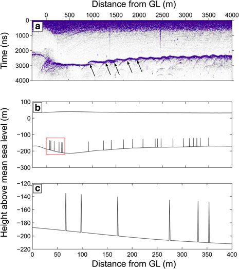
Rosier and others: On the interpretation of ice-shelf flexure measurements                                                                               785

       where eij are the components of the strain tensor and δij is the                         we do not expand on this analysis. We briefly show the
       Kronecker Delta.                                                                         effect of reducing k in one set of experiments for the sake
          Ice is treated as a Maxwell viscoelastic material. This is a                          of comparison, but in general k is fixed to a value of 1 GPa
       two-element rheological model comprising a viscous                                       m−1, representing a relatively stiff bed (Sayag and Worster,
       damper and an elastic spring connected in series, such that                              2013) to avoid complicating our results with soft till effects.
       an applied stress yields an instantaneous elastic strain and                             At the GL ice is pinned to the bed such that the GL cannot
       a time dependent viscous strain. The total deviatoric strain                             migrate, in accordance with DInSAR analysis that shows no
       rate e_ ij is therefore the sum of these two contributions:                              GL migration at this site (Wild and others, 2017). The GL pos-
                                                                                                ition used in the model is the GL position as identified in the
                                                         1 ∇
                                  e_ ij ¼ Aτ n1
                                             E τ ij þ      τ ij ;                     ð6Þ       radargram with the aid of DInSAR interferograms.
                                                        2G                                          It is worth pointing out here that, although the system of
       where the dot indicates a time derivative.                                               equations we solve in our model are very different from the
          The first term on the right-hand side represents the viscous                          purely elastic beam model, the boundary conditions we
       component of deformation where A is the temperature                                      employ are almost exactly the same. In his derivation,
       dependent rate factor in Glen’s flow law, n is creep exponent                            Holdsworth (1969) assumes that the ice is plane strain,
       (a nonlinear relation with n = 3 is used throughout) and                                 resting on an elastic foundation and clamped vertically at
                                                                                                the GL. At the downstream end of the beam the vertical
                                      qffiffiffiffiffiffiffiffiffiffiffiffiffiffi
                                                                                                deflection equals vertical tidal motion and its gradients in x
                                τ E ¼ τ ij τ ji =2                 ð7Þ
                                                                                                are zero. All these conditions are satisfied in our model, pro-
                                                                                                vided that the domain is sufficiently long (which we show
       is the effective stress. The second term on the right-hand side                          later in the results).
       of (6) is the elastic component of deformation, where the                                    The model domain consists of an unstructured mesh of
       superscript ∇ denotes the upper-convected time derivative:                               ∼50,000, 2-D isoparametric triangular elements, refined
                                                                                                around the grounding zone leading to a resolution of up to
                              ∇       D         ∂vi        ∂vj
                             τ ij ¼      τ ij      τ kj      τ ik ;                 ð8Þ       4 m in this region. Radargrams in this area, obtained during
                                      Dt        ∂xk        ∂xk                                  a recent survey, indicate extensive basal crevassing in the
                                                                                                grounding zone. In some simulations we manually add
       G is the shear modulus:
                                                                                                cracks into the finite element mesh at locations where we
                                                 E                                              interpret likely basal crevasses based on one of the radar-
                                        G¼             ;                              ð9Þ       grams across the White Island grounding zone (Fig. 2a).
                                              2ð1 þ nÞ

       ν is the Poisson’s ratio and E is the Young’s modulus
       (Christensen, 1982). A standard value of 0.3 is used through-
       out for the Poisson’s ratio (Lingle and others, 1981;
       Stephenson, 1984; Kobarg, 1988; Smith, 1991; Vaughan,
       1995; Schmeltz and others, 2002; Sykes and others, 2009)
       and in line with previous studies the effect of changing this
       is negligible and not discussed further.
           We choose to avoid the complication of matching the
       background flow of the ice stream, largely because the
       flow in this region is not aligned with the 2-D flexure line
       that we investigate. Following Thompson and others (2014)
       we set the body force fi = 0 in (2). This will only alter the
       viscous component of our model since the effective viscosity
       is a function of the effective stress. In this case, since we are
       only interested in the relative amplitude of the flexure profile
       and do not investigate its phase, any resulting difference
       between the two models will be very small. Without the
       body force there is no need to apply an ocean back pressure
       at the downstream end of the model, so instead a stress-free
       condition is applied.
           Ice rests on seawater of uniform mass density ρw = 1030
       kg m−3 ,which exerts an ocean pressure normal to the base
       of the floating ice shelf given by

                                        pw ¼ ρw gSðtÞ;                              ð10Þ        Fig. 2. (a) Radargram across the grounding zone of White Island,
                                                                                                Southern McMurdo Ice Shelf, showing extensive basal crevassing
                                                                                                (some of the more distinct basal crevasses are indicated by
       where g is gravitational acceleration, S(t) is the time varying
                                                                                                arrows). (b) Outline of the model domain in the grounding zone
       sea level, consisting of a sine wave of diurnal period with
                                                                                                for a crevassed geometry: a = 0.25 H, α = 1°, where a is the
       an amplitude equal to the local ocean tide of ∼0.3 m.                                    crevasse depth through the ice thickness H and α is the crevasse
       Grounded ice rests on an elastic bed 5 m thick with stiffness                            opening angle. Note that the full model domain extends beyond
       k = Et/Ht, where Et is the till elasticity and Ht is the till thick-                     this region (extent shown in Fig. 1). (c) Close up of the portion of
       ness. Sayag and Worster (2011, 2013) previously investi-                                 the domain outlined in the red box of panel b, showing details of
       gated the effects of till stiffness on the flexure profile and                           the crevasse geometry for α = 1°.

Downloaded from https://www.cambridge.org/core. 23 Jan 2021 at 20:00:37, subject to the Cambridge Core terms of use.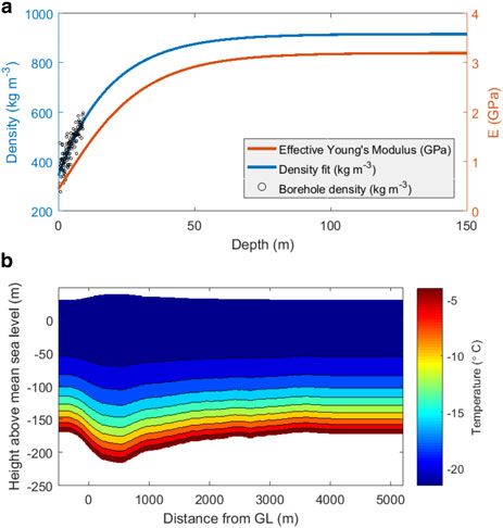
786 Rosier and others: On the interpretation of ice-shelf flexure measurements
Due to the difficulty in determining crevasse depths from the however the firn stiffness will undoubtedly be lower and so
radargram we adopt the simpler approach of testing two this simplest approach provides a useful first step in investi-
scenarios, with depths chosen to be either 10% or 25% of gating how the flexure profile would change as a result of
local ice thickness and crack opening angles (α) of either reduced surface stiffness.
1° or 0.001°. An outline of the resulting model geometry, A temperature distribution was taken from recent mea-
showing crevasse depths of 25% ice thickness and crack surements made in a nearby portion of the McMurdo Ice
opening angles of 1°, is shown in Fig. 2b. Shelf (Kobs and others, 2014) and applied to the model
A 10 m firn core was taken in the survey area at the same with the simplifying assumption that there is no lateral vari-
time as radar measurements were made (location shown in ation in basal temperature (Fig. 3b). The rate factor A is
Fig. 1). This was divided into 5–10 cm sections, which then made a function of temperature using the relation
were weighed and measured to obtain estimates of firn densi- derived by Smith (1981).
fication (shown in Fig. 3a). These measurements were fitted
to an exponential curve assuming glacial ice mass density
(ρice) of 917 kg m−3 giving the following depth density rela- 3. RESULTS
tion: Our results are divided into two sections; firstly we use the
full-Stokes viscoelastic model described in Section 2 to simu-
ρi ðzÞ ¼ ρice ð573 expð0:0529zÞÞ: ð11Þ
late ice flexure for a number of different geometries and par-
ameter choices to show the effect of these changes on the
Along with the mass density profile given in (11) we use a surface flexure signal. We then use a nonlinear regression
simple relation of a form given by Gibson and Ashby (1988) to fit an analytical elastic beam solution to our modelled
to calculate a depth dependent Young’s modulus as flexure profiles in order to evaluate the performance of this
technique and discuss what can be gained from such an
exercise.
ρi ðzÞ 2
EðzÞ ¼ Eice : ð12Þ
ρice
The resulting profiles for mass density and Young’s modulus 3.1. Full-stokes model
are shown in Fig. 3a. To make for a sensible comparison Eice We begin by presenting results from a control run, whereby
is chosen to be 3.2 GPa so that the Young’s modulus of we use the full-Stokes viscoelastic model to calculate a
glacial ice remains the same as that of the control simulation flexure profile but without any additional perturbations i.e.
and the only difference is in the stiffness of the firn layer. not changing Young’s modulus with depth and using a
Using this relation the depth averaged E becomes 2.9 GPa, mesh without crevasses. Model simulations use a time
however the change is not that simple given that the stiffness varying sea level (10) and the flexure profile is the difference
is only reduced at the ice surface. A variety of relations between the surface elevation at high tide and the surface
between mass density and stiffness exist and no measure- with no tide. We approach this control run in the same
ments were made with which to test this particular form, way as previous studies, by taking the thickness profile and
tuning the Young’s modulus to match an observed flexure
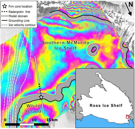
profile measured by differential interferometry. Figure 4
shows the DInSAR flexure profile (blue line) and the best fit
obtained with an effective Young’s modulus of 3.2 GPa
(black line) i.e. the control run. As a next step, we introduce
basal crevasses with depths of 25% ice thickness into the
mesh as described in Section 2 and rerun the model. In this
Fig. 3. (a) Density relation obtained by fitting an exponential curve
(11) (blue line) to firn density measurements obtained with the 10 m Fig. 4. DInSAR flexure profile (blue curve) compared with best fits
core (circles) and the resultant variation in Young’s modulus with for the crevassed and control geometries (red and black lines,
depth as determined from (12) (red line). (b) Temperature respectively). Both modelled curves are outputs from the full-
distribution used in the model. Stokes viscoelastic model.
Downloaded from https://www.cambridge.org/core. 23 Jan 2021 at 20:00:37, subject to the Cambridge Core terms of use.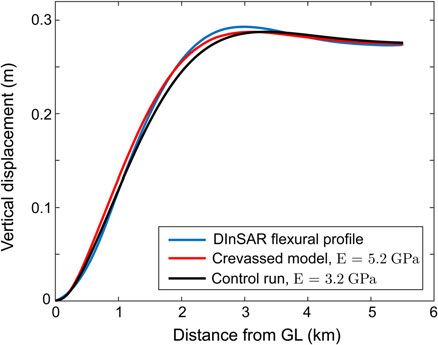
Rosier and others: On the interpretation of ice-shelf flexure measurements 787
case the effective Young’s modulus needed to match obser-
vations is 5.2 GPa (Fig. 4, red line).
Figure 5 shows the difference between the control run
and a more complete set of experiments. To aid comparison
we include results of two simulations where the only
change was to increase or decrease the Young’s modulus
of ice by ±25 % to 4.0 and 2.4 GPa, respectively (Fig. 5a).
The first experiment (yellow line in Fig. 5a) uses the
density profile shown in Fig. 3 (blue line) to reduce near-
surface ice elasticity according to the relation given by
(12) (denoted E = f(ρi)). The effect is similar to reducing
the overall Young’s modulus of the entire ice shelf by
25% with no clear way to differentiate between the two
cases.
Comparison of results between experiments that intro-
duced basal crevasses into the model domain are shown in
Fig. 5b. Where the crack opening angle is large (α = 1°)
there is no difference between the flexure profiles at high
and low tide (low tide profiles overlap exactly with their
respective high tide profiles and so are not included) .
For cracks that penetrate 25% of ice thickness the effect
on the flexure profile is very large, equivalent to a reduc-
tion of Young’s modulus of 40%. The effect for cracks
that penetrate 10% of ice thickness is smaller but still
important.
Where the crack opening angle is very small (α = 0.001°)
there is a difference between the flexure profile at high and
low tide (low tide flexure profiles are inverted and indicated
by dashed lines). This is because the cracks are sufficiently
narrow that at various stages in the tidal cycle cracks in a
compression region might close fully at which point they
no longer reduce the effective stiffness of the ice. This
happens at different phases of the tide for different cracks
and also explains why the overall effect of these cracks is
smaller than for large opening angles.
In a number of previous studies it is assumed that ice rests
on an elastic bed (Sayag and Worster, 2013; Walker and
others, 2013) and so we also include the effect of reducing
the stiffness of the bed (Fig. 5c). This has a similar influence
on the flexure profile as reducing the effective ice stiffness
but also increases the reversed sign deflection upstream of
the grounding line.
Several tests were performed to check that the 15 km
length of floating shelf was sufficiently long. Due to the
stress free boundary condition at the downstream end of
the model, if the domain is much longer than the character-
istic bending lengthscale (in this case 1/β ≈ 1 km) then the
solution will approach that of an infinitely long ice shelf.
Fig. 5. Difference in flexure profile between the control (E = 3.2 Doubling the length of the ice shelf to 30 km for the a =
GPa, k = 103 MPa, no crevasses) and various experimental setups. 25 H, α = 1° geometry led to a maximum difference
(a) shows the effect of making Young’s modulus a function of ice
between the two resulting profiles of 2 × 10⁻⁵ m. Since this
mass density, denoted E = f(ρi) along with the most extreme
scenario tested, with crevasse depths of 25% ice thickness and
difference is three orders of magnitude smaller than the
density dependent E. Difference in flexure profile obtained by signals we investigate, we consider our domain to be suffi-
simply altering the Young’s modulus are included for the sake of ciently large that boundary effects are negligible.
comparison (b) shows the difference with crevassed geometries of
crevasse depths 0.1 and 0.25 H and crevasse opening angles α =
1° and α = 0.001°. Dashed lines in panel b indicate the equivalent 3.2. Elastic beam fitting
difference in flexure profile at low tide. Note that for large crack
opening angles α = 1° low tide profiles overlap exactly with their We now attempt to fit an analytical elastic beam solution to
respective high tide profiles and so are not shown. (c) shows the our modelled flexure profiles to evaluate its performance and
change in flexure profile as the bed is made more elastic, from ability to provide useful information on elasticity and GL pos-
k = 102 MPa to k = 100 MPa. All curves shown are outputs from ition. Following a similar approach to Rignot (1998a), we
the viscoelastic full-Stokes model. assume an elastic tidal flexure profile for a positive vertical
Downloaded from https://www.cambridge.org/core. 23 Jan 2021 at 20:00:37, subject to the Cambridge Core terms of use.788 Rosier and others: On the interpretation of ice-shelf flexure measurements
deflection of 1 m that takes the form summarised in Table 1. For the most extreme experiment,
where we introduce basal crevasses with a depth of 0.25 H
1 expðβx0 Þ½cosðβx0 Þ þ sinðβx0 Þ x > x0 and make Young’s modulus a function of mass density, the
yðxÞ ¼ ð13Þ
0 x x0 elastic beam model finds a best fit for E = 1.47 GPa i.e.
over a factor of two error from the actual Young’s modulus
(Holdsworth, 1969) where x′ = x − x0, x0 is the estimated GL used. The elastic beam model fit to profiles produced by
position and the full-Stokes model was good in all cases, with typical
RMSE of ∼2–3 mm.
1=4
1 n2 Various approaches have been used in the past to estimate
β¼ 3ρw g ð14Þ GL position from SAR interferometry. Some previous studies
Eh3
fit an elastic beam model to the DInSAR flexure profile and
is the spatial wavenumber. We apply a nonlinear regression assign the upper limit of tidal flexure (F) at the point x0
(e.g. Dennis and Schnabel, 1996) of the form (Rignot, 1998a, b; Sykes and others, 2009). Alternatively,
the assumed GL position (G) is placed at the point that verti-
ðkþ1Þ ðkÞ ðkÞ ðkÞ ðkÞ ðkÞ
bi ¼ bi þ ðK ji K jk Þ1 Kkl ðy^l yl Þ; ð15Þ cal motion of ice is detected for the first time above noise
level in the interferogram. We replicate the fringe picking
where approach by differencing two modelled flexure profiles at
random points in the tidal cycle and placing G where the
β flexure exceeds 2.2 cm, ie. the height equivalent to one inter-
b¼ ; ð16Þ ferogram fringe in TerraSAR-X interferograms. This is repeated
xo
1000 times for each experiment, discarding any sampling
dyi where the difference in tidal elevation wasRosier and others: On the interpretation of ice-shelf flexure measurements 789
grounding line. The two approaches tested here appear to Since there is no consensus on an appropriate temperature-
perform reasonably well, differing from the true GL position elasticity relation for glacial ice and any changes to ice stiff-
by ∼80–150 m, however there are two caveats to this. ness would be slight, we choose to ignore this effect. A more
Firstly the geometry used in this work can be considered an important effect of temperature is likely the change in viscos-
ideal case, with no lateral effects and a steep bed slope, so ity, which shows a clearer and stronger dependence on tem-
the accuracy of the GL position is likely a best case scenario. perature. Warmer ice is less viscous and so it might be that
Shallower bed slopes in particular would likely lead to larger ice behaves more viscoelastically over tidal timescales at
discrepancies between either F or G and the true GL position. its base and more elastically at the surface.
Secondly it is worth noting that, taking this domain as an Tidal migration of the grounding line was not included in
example, an error in GL position of 150 m would result in the viscoelastic model presented here because the lack of a
an error in ice thickness at the GL of over 8%. body force to balance ocean pressure forcing the ice off the
Errors in the regression were always small, implying that a bed results in limitless upstream migration on the high tide.
simple elastic beam model can be made to fit very well to a In order to check the influence of this the model was run
flexure profile with only two fitting parameters. These small with the local tidal amplitude and the body force included,
errors are often cited in previous studies to provide confi- allowing the grounding line to migrate for a purely elastic
dence in this type of approach (Vaughan, 1995; Rignot, ice rheology, and compared with results with a fixed ground-
1998a, b) however it is clear that care must be taken if this ing line. Due to the very steep bedrock topography in the
approach is used to estimate either H or E since other grounding zone of the White Island transect that we model,
factors might be at play. In fact, since it is only the product migration of the grounding line was only Oð1 mÞ and
of EH3 that enters (14) (Holdsworth, 1969), it is impossible hence the effect on the flexure profile was negligible.
to independently estimate E or H without having some add- Clearly on shallow sloping beds where tidal migration of
itional information. It is worth noting that, although a model the grounding line is potentially as much as several kilo-
based on the elastic beam approximation will never succeed meters (Brunt and others, 2011) the effect will be very consid-
in capturing this additional level of complexity, any model erable and the assumption of a fixed grounding line for either
(i.e. viscoelastic) may lead to a misinterpretation of a an elastic beam model or the full-Stokes model presented
flexure profile without prior knowledge of factors such as here would lead to an articially narrow grounding zone.
basal crevasses and mass density distribution. Walker and others (2013) treat the GL as a fulcrum which,
We can use this same product of EH3 in (14) to explore a while it may be a suitable simplification for analysing tidal
first order estimate of what the change in effective ice stiffness flexure, is implausible based on the known physical proper-
due to crevasses using elastic beam theory would be. In the ties of ice and from geometrical considerations (Tsai and
case of crevasses that penetrate to 25% of the ice thickness, Gudmundsson, 2015). The limited evidence of reversed
this can be thought of in a most basic sense as reducing the flexure upstream of the grounding line can be explained
effective ice thickness by the same amount. Using this physically without this fulcrum if ice is resting on a soft till
simple approach and the EH3 relation, a 25% reduction in as shown in our experiments (Fig. 5c) and previously by
ice thickness would be expected to manifest itself as a reduc- Sayag and Worster (2011, 2013). The recent use of a
tion in the effective ice stiffness of almost 60%. Using the full- fulcrum as a mechanism to drive warm water upstream into
Stokes model we find the actual reduction to be closer to the subglacial water system and speed up ice retreat
40% (Fig. 4). This discrepancy is unsurprising because the (Parizek and others, 2013) is therefore inappropriate. It has
ice in our model is not completely crevassed along its been shown that change to the subglacial hydraulic potential
entire length and so a lot of ice remains to provide bending due to ice flexure would not lead to suction of ocean water
resistance between crevasses. This difference highlights far upstream of the grounding line (Sayag and Worster,
once again the dangers in applying the linear elastic beam 2013).
theory far beyond its useful bounds.
Small surface strand cracks were observed in the ground-
ing zone but are not visible in the radar profiles and so they 5. CONCLUSIONS
have not been included in the cracked model domain. Observations of tidal flexure in the grounding zone have
Including strand cracks would further alter the bending been used extensively in previous studies to determine
profile, although since strand cracks reduce the stiffness of approximate grounding line position and ice properties.
the less dense firn layer this effect is likely to be smaller We have shown, using a viscoelastic full-Stokes model of
than basal crevasses. flexure constrained by observations made in the grounding
Nearby thermal profiles of the Southern McMurdo ice zone of the McMurdo ice shelf, that the interpretation of
shelf found temperatures of ∼ 20 ○ C at the ice surface, flexure measurements could vary considerably depending
increasing to ∼ 4 ○ C at the base with an approximately on the modeling assumptions made. Inclusion of observed
exponential profile (Kobs and others, 2014). Laboratory basal crevasses and mass density dependent elasticity alters
experiments investigating the temperature dependence of the effective Young’s modulus obtained by fitting the
ice elasticity show that warmer temperatures lead to model to the observed flexure by up to 200% in the set of
reduced stiffness but do not find a clear relation that can be experiments presented here. Conversely, estimates of GL
applied to our model (Hobbs, 1974; Schulson and Duval, position are reasonably accurate although this may be
2009). Based on the experiments of Dantl (1968) a tempera- partly fortuitous as a consequence of the large gradients in
ture change of ∼20 ○ C would result in only a ∼3% change in geometry at the GL.
ice stiffness whereas experiments by Jellinek and Brill (1956) No previous model has included all of the processes
suggest a larger sensitivity but with no clear trend. Schulson investigated here and yet the misfit between these previous
and Duval (2009) suggest that a temperature range 0 50 ○ C models and observations is always small unless ice thickness
causes the effective stiffness of ice to change by only 5%. is poorly known. Factors such as extensive crevassing might
Downloaded from https://www.cambridge.org/core. 23 Jan 2021 at 20:00:37, subject to the Cambridge Core terms of use.790 Rosier and others: On the interpretation of ice-shelf flexure measurements
be expected to change the shape of a flexure profile suffi- periodic crevasses. Ann. Glaciol., 53(60), 85–89 (doi: 10.3189/
ciently that a linear elastic beam model would no longer 2012AoG60A120)
provide a good fit and yet our results show that this is not Gibson LG and Ashby MF (1988) Cellular solids: structure and prop-
the case and misfit remained small in all cases. The goodness erties. Pergamon Press, Oxford, UK
Goldstein RM, Engelhardt H, Kamb B and Frolich RM (1993)
of fit obtained by the beam theory does not imply that the
Satellite radar interferometry for monitoring ice sheet motion:
rheological description on which it is based is correct but is
application to an Antarctic ice stream. Science, 262(5139),
a consequence of fitting only the amplitude of the flexure 1525–1530 (doi: 10.1126/science.262.5139.1525)
curve. Deriving values for the Young’s modulus in this Gudmundsson GH (2006) Fortnightly variations in the flow velocity
manner and comparing with laboratory derived values, as of Rutford Ice Stream, West Antarctica. Nature, 444(7122),
has been done in numerous previous studies, does not 1063–1064 (doi: doi:10.1038/nature05430)
provide satisfactory insight into the relevant ice rheology. Gudmundsson GH (2007) Tides and the flow of Rutford Ice Stream,
In addition, the derived rheological parameters are not trans- West Antarctica. J. Geophys. Res., 112, F04007 (doi: 10.1029/
ferrable to other ice streams where local conditions might be 2006JF000731)
completely different. An elastic beam model will also fail to Gudmundsson GH (2011) Ice-stream response to ocean tides and
reproduce the phase relationship between tides and stresses the form of the basal sliding law. Cryosphere, 5(1), 259–270
(doi: 10.5194/tc-5-259-2011)
acting at the grounding line, and such an approach is not suit-
Hobbs PV (1974) Ice physics. Oxford University Press, Ely House,
able for studies of tidal modulation on ice streams. These London
results imply that extreme caution should be used when Holdsworth G (1969) Flexure of a floating ice tongue. J. Glaciol., 8,
fitting models to flexure profiles to estimate either E or H 133–397
since many other factors could be at play. Holdsworth G (1977) Tidal interaction with ice shelves. Ann.
Geophys., 33, 133–146
Hulbe CL and 5 others (2016) Tidal bending and strand cracks at the
Kamb ice stream grounding line, west Antarctica. J. Glaciol., 62
ACKNOWLEDGEMENTS (235), 816–824 (doi: 10.1017/jog.2016.74)
S. Rosier was supported by a SCAR fellowship grant for a Hutter K (1983) Theoretical glaciology: material science of ice and
research stay at Gateway Antarctica, University of the mechanics of glaciers and ice sheets. Mathematical
Canterbury, Christchurch, New Zealand, and the NERC Approaches to Geophysics, D. Reidel Publishing Company,
large grant ‘Ice shelves in a warming world: Filchner Ice Dordrecht, Holland, ISBN 9789027714732
Shelf System’ (NE/L013770/1). Field data were collected in Jellinek HHG and Brill R (1956) Viscoelastic properties of ice.
J. Appl. Phys., 27(10), 1198–1209 (doi: 10.1063/1.1722231)
2014 during the NZARI project ‘Tidal flexure of ice
Kobarg W (1988) The tide-dependent dynamics of the Ekström ice
shelves’ and supported by Antarctica NZ. TerraSAR-X satel-
shelf, Antarctica. Berichte zur Polarforschung, Alfred-Wegener-
lite data for the InSAR analysis have been acquired by DLR Inst. für Polar- u. Meeresforsch., Bremerhaven, Germany
(project HYD1421) during the same field work within that Kobs S, Holland DM, Zagorodnov V, Stern A and Tyler SW (2014)
project. Landsat 8 data available from the US Geological Novel monitoring of Antarctic ice shelf basal melting using a
Survey. We are grateful to R. Greve and two anonymous fiber-optic distributed temperature sensing mooring. Geophys.
reviewers whose comments greatly improved the quality of Res. Lett., 41(19), 6779–6786 (doi: 10.1002/2014GL061155)
this manuscript. Lingle CS, Hughes TJ and Kollmeyer RC (1981) Tidal flexure of
jakobshavns glacier, west Greenland. J. Geophys. Res.: Sol.
Ea., 86(B5), 3960–3968 (doi: 10.1029/JB086iB05p03960)
Marsh OJ, Rack W, Golledge NR, Lawson W and Floricioiu D (2014)
REFERENCES Grounding-zone ice thickness from insar: inverse modelling of
Anandakrishnan S, Voigt DE and Alley RB (2003) Ice stream D flow tidal elastic bending. J. Glaciol., 60(221), 526–536 (doi:
speed is strongly modulated by the tide beneath the Ross 10.3189/2014JoG13J033)
Ice Shelf. Geophys. Res. Lett., 30(7), 1361 (doi: 10.1029/ MSC (2016) Marc 2016 volume A: theory and user information.
2002GL016329) MSC MARC, MSC Software Corporation, 2 MacArther Place,
Bindschadler RA, King MA, Alley RB, Anandakrishnan S and Santa Ana, CA 92707
Padman L (2003) Tidally controlled stick-slip discharge of a Parizek BR and 10 others (2013) Dynamic (in)stability of thwaites
West Antarctic ice stream. Science, 301, 1087–1089 (doi: glacier, west Antarctica. J. Geophys. Res.: Ea. Surf., 118(2),
10.1126/science.1087231) 638–655, ISSN 2169-9011 (doi: 10.1002/jgrf.20044)
Borstad CP and 6 others (2012) A damage mechanics assessment of Petrenko V and Whitworth R (2002) Physics of ice. Oxford
the larsen b ice shelf prior to collapse: toward a physically-based University Press, Oxford
calving law. Geophys. Res. Lett., 39(18), L18502 (doi: 10.1029/ Pralong A and Funk M (2005) Dynamic damage model of crevasse
2012GL053317) opening and application to glacier calving. J. Geophys. Res.:
Brunt KM, Fricker HA and Padman L (2011) Analysis of ice plains Sol. Ea., 110(B1), B01309, ISSN 2156-2202 (doi: 10.1029/
of the filchner-ronne ice shelf, Antarctica, using icesat laser 2004JB003104)
altimetry. J. Glaciol., 57(205), 965–975 Pralong A, Funk M and Lüthi MP (2003) A description of Crevasse
Christensen RM (1982) Theory of viscoelasticity. 2nd edn. Academic formation using continuum damage mechanics. Ann. Glaciol.,
Press, New York 37, 77–82 (doi: 10.3189/172756403781816077)
Dantl G (1968) Die elastischen moduln von eis-einkristallen. Physik Reeh N, Christensen EL, Mayer C and Olesen OB (2003) Tidal
der kondensierten Materie, 7(5), 390–397 (doi: 10.1007/ bending of glaciers: a linear viscoelastic approach. Ann.
BF02422784) Glaciol., 37, 83–89 (doi: 10.3189/172756403781815663)
Dennis J and Schnabel R (1996) Numerical methods for uncon- Rignot EJ (1998a) Hinge-line migration of petermann gletscher,
strained optimization and nonlinear equations. Society for north Greenland, detected using satellite-radar interferometry.
Industrial and Applied Mathematics, Philadelphia, PA, USA J. Glaciol., 44, 469–476
(doi: 10.1137/1.9781611971200) Rignot EJ (1998b) Radar interferometry detection of hinge-line
Freed-Brown J, Amundson JM, MacAyeal DR and Zhang WW (2012) migration on rutford ice stream and carlson inlet, Antarctica.
Blocking a wave: frequency band gaps in ice shelves with Ann. Glaciol., 27, 25–32
Downloaded from https://www.cambridge.org/core. 23 Jan 2021 at 20:00:37, subject to the Cambridge Core terms of use.Rosier and others: On the interpretation of ice-shelf flexure measurements 791
Rignot EJ, Mouginot J and Scheuchl B (2011) Antarctic grounding Smith AM (1991) The use of tiltmeters to study the dynamics of
line mapping from differential satellite radar interferometry. Antarctic ice-shelf grounding lines. J. Glaciol., 37(125), 51–58
Geophys. Res. Lett., 38(10), l10504, ISSN 1944-8007 (doi: Smith GD (1981) Viscous relations for the steady creep of polycrys-
10.1029/2011GL047109) talline ice. Cold Reg. Sci. Technol., 5, 141–150
Rist MA and 5 others (1996) Experimental fracture and mechanical prop- Stephenson SN (1984) Glacier flexure and the position of grounding
erties of Antarctic ice preliminary results. Ann. Glaciol., 23, 284–292 lines: measurements by tiltmeter on Rutford Ice Stream
Roethlisberger H (1972) Seismic exploration in cold regions. CRREL Antarctica. Ann. Glaciol., 5, 165–169
monograph, U.S. Army Cold Regions Research and Engineering Sykes HJ, Murray T and Luckman A (2009) The location of the
Laboratory, Hanover, NH, USA grounding zone of Evans ice stream, Antarctica, investigated
Rosier SHR and Gudmundsson GH (2016) Tidal controls on the flow using sar interferometry and modelling. Ann. Glaciol., 50(52),
of ice streams. Geophys. Res. Lett., 43(9), 4433–4440, ISSN 35–40 (doi: doi:10.3189/172756409789624292)
1944-8007 (doi: 10.1002/2016GL068220) Thompson J, Simons M and Tsai VC (2014) Modeling the elastic
Rosier SHR, Gudmundsson GH and Green JAM (2014) Insights into transmission of tidal stresses to great distances inland in channe-
ice stream dynamics through modeling their response to tidal lized ice streams. Cryosphere, 8, 2007–2029 (doi: 10.5194/tc-8-
forcing. Cryosphere, 8, 1763–1775 (doi: 10.5194/tc-8-1763-2014) 2007-2014)
Rosier SHR, Gudmundsson GH and Green JAM (2015) Temporal Tsai VC and Gudmundsson GH (2015) An improved model for
variations in the flow of a large Antarctic ice-stream controlled tidally-modulated grounding line migration. J. Glaciol., 61
by tidally induced changes in the subglacial water system. (226), 216–222 (doi: 10.3189/2015JoG14J152)
Cryosphere, 9, 1649–1661 (doi: 10.5194/tc-9-1649-2015) Tsai VC, Rice JR and Fahnestock M (2008) Possible mechanisms for
Sayag R and Worster GM (2011) Elastic response of a grounded ice glacial earthquakes. J. Geophys. Res.: Ea. Surf., 113(F3), f03014,
sheet coupled to a floating ice shelf. Phys. Rev. E, 84, 036111 ISSN 2156-2202 (doi: 10.1029/2007JF000944)
(doi: 10.1103/PhysRevE.84.036111) Vaughan DG (1995) Tidal flexure at ice shelf margins. J. Geophys.
Sayag R and Worster GM (2013) Elastic dynamics and tidal migration Res., 100, 6213–6224
of grounding lines modify subglacial lubrication and melting. Walker RT, Christianson K, Parizek BR, Anandakrishnan S and
Geophys. Res. Lett., 40, 5877–5881 (doi: 10.1002/2013GL057942) Alley RB (2012) A viscoelastic flowline model applied to tidal
Schmeltz M, Rignot EJ and MacAyeal D (2002) Tidal flexure along forcing of bindschadler ice stream, west Antarctica. Earth
ice-sheet margins: comparison of insar with an elastic-plate Planet Sci. Lett., 319–320, 128–132 (doi: 10.1016/j.
model. Ann. Glaciol., 34(1), 202–208 (doi: 10.3189/ epsl.2011.12.019)
172756402781818049) Walker RT and 5 others (2013) Ice-shelf tidal flexure and subglacial
Schulson EM and Duval P (2009) Creep and fracture of ice. pressure variations. Earth Planet Sci. Lett., 361, 422–428 (doi:
Cambridge University Press, Cambridge CB2 8RU, UK 10.1016/j.epsl.2012.11.008)
Shepherd A and 46 others (2012) A reconciled estimate of ice-sheet Wild CT, Marsh OJ and Rack W (2017) Viscosity and elasticity: a
mass balance. Science, 338(6111), 1183–1189 (doi: 10.1126/ model-intercomparison of ice-shelf bending in an Antarctic
science.1228102) grounding zone. J. Glaciol., 15, 1–8 (doi: 10.1017/jog.2017.15)
MS received 16 August 2016 and accepted in revised form 13 July 2017; first published online 22 August 2017
Downloaded from https://www.cambridge.org/core. 23 Jan 2021 at 20:00:37, subject to the Cambridge Core terms of use.You can also read