A new description of probability density distributions of polar mesospheric clouds
←
→
Page content transcription
If your browser does not render page correctly, please read the page content below

Atmos. Chem. Phys., 19, 4685–4702, 2019
https://doi.org/10.5194/acp-19-4685-2019
© Author(s) 2019. This work is distributed under
the Creative Commons Attribution 4.0 License.

A new description of probability density distributions
of polar mesospheric clouds
Uwe Berger, Gerd Baumgarten, Jens Fiedler, and Franz-Josef Lübken
Leibniz-Institute of Atmospheric Physics, Rostock University, Kühlungsborn, Germany

Correspondence: Uwe Berger (berger@iap-kborn.de)

Received: 27 June 2018 – Discussion started: 20 July 2018
Revised: 8 November 2018 – Accepted: 12 November 2018 – Published: 8 April 2019

Abstract. In this paper we present a new description of sta-       the Nimbus-7 satellite over the period 1978–1986, measur-
tistical probability density functions (pdfs) of polar meso-       ing scattered limb albedo at 265 nm and nadir albedo at
spheric clouds (PMCs). The analysis is based on observa-           273.5 nm, respectively. Thomas (1995) introduced empirical
tions of maximum backscatter, ice mass density, ice particle       measures in the statistical analysis of PMC brightness distri-
radius, and number density of ice particles measured by the        butions. He showed that the frequency distribution of PMC
ALOMAR Rayleigh–Mie–Raman lidar for all PMC seasons                albedo derived from both SME and SBUV satellite data can
from 2002 to 2016. From this data set we derive a new class        be approximated by an (normalized) exponential probability
of pdfs that describe the statistics of PMC events that is dif-    function, see Fig. 3 in Thomas (1995). Secondly, the author
ferent from previous statistical methods using the approach        also proposed to use cumulative frequency numbers (the so-
of an exponential distribution commonly named the g distri-        called g function) of clouds, g(A), exceeding a certain albedo
bution. The new analysis describes successfully the proba-         A in order to better represent the exponential populations.
bility distributions of ALOMAR lidar data. It turns out that       Examples of g distributions are plotted on a semilogarithmic
the former g-function description is a special case of our new     scale in Fig. 4 in Thomas (1995), clearly indicating an ap-
approach. In general the new statistical function can be ap-       proximately linear behavior of cumulative frequencies in a
plied to many kinds of different PMC parameters, e.g., max-        logarithmic format.
imum backscatter, integrated backscatter, ice mass density,           In the following years many observational PMC analyses
ice water content, ice particle radius, ice particle number den-   of seasonal statistics have been published frequently using
sity, or albedo measured by satellites. As a main advantage        the g function, e.g., reports from Wind Imaging Interferome-
the new method allows us to connect different observational        ter (WINDII) and Polar Ozone and Aerosol Measurement II
PMC distributions of lidar and satellite data, and also to com-    data (Shettle et al., 2002), SBUV data (Deland et al., 2003),
pare with distributions from ice model studies. In particular,     Student Nitric Oxide Explorer (SNOE) data (Bailey et al.,
the statistical distributions of different ice parameters can be   2007), ice water content data derived from SBUV (DeLand
compared with each other on the basis of a common assess-          and Thomas, 2015), or ALOMAR lidar data (Fiedler et al.,
ment that facilitates, for example, trend analysis of PMC.         2017). Also model analyses have used the g function inves-
                                                                   tigating trends and long-term changes in PMC parameters
                                                                   (Lübken et al., 2013; Berger and Lübken, 2015).
                                                                      The g-function approach has been relatively successfully
1   Introduction                                                   applied to many kinds of different PMC parameters as
                                                                   brightness, albedo, maximum backscatter ratio, integrated
First studies of probability distributions of polar mesospheric    backscatter, ice water content, ice mass densities, ice parti-
clouds (PMCs) were reported by Thomas (1995) using data            cle size, or ice particle number density since frequency his-
from the UVS (ultraviolet spectrograph) instrument on board        tograms of all these parameters have sometimes a nearly, at
the Solar Mesosphere Explorer (SME) satellite and from             least piecewise, exponential shape. Furthermore, sometimes
the Solar Backscatter Ultraviolet (SBUV) instrument on

Published by Copernicus Publications on behalf of the European Geosciences Union.
4686                                                              U. Berger et al.: Probability density distributions of PMC

PMC data seem to fit almost perfectly to exponential distri-      evidence of Gaussian-distributed ice particles at the height
butions, particularly when using cumulative standardizations      of maximum brightness of PMC, e.g., Berger and von Zahn
of data (Thomas, 1995). An example of a good exponential          (2002) and Rapp and Thomas (2006).
fit is the frequency distribution of ALOMAR backscatter data         In this paper we will analyze the climatology of all ice
that are discussed in Sect. 3.1.1. On the other hand, in some     seasons from 2002 until 2016 merging all 15 seasons to one
statistical applications it is obvious that the exponential ap-   data record. Within this combined data set we then get a total
proach describes the data rather insufficiently, see examples     number N of 8597 observations, which is sufficiently numer-
of ice mass density, ice radius, and ice number density in        ous in order to avoid excessive statistical irregularities in a
Sect. 3.1.2. Therefore it is a desirable task to provide some     frequency histogram of the data.
more aspects on the theory of PMC statistics.
    This paper makes an attempt to investigate in more de-
tail the statistics of probability density functions (pdfs) of    3   The exponential probability distribution (g function)
PMC climatology for various ice parameters. In the follow-
                                                                  In general, the seasonal climatology of PMC events with
ing we analyze a PMC data record of maximum backscatter,
                                                                  measured ice parameters, such as integrated backscatter,
ice mass density, ice particle radius, and number density from
                                                                  maximum backscatter, column ice mass, albedo, or ice mass
the period 2002–2016 measured by the ALOMAR Rayleigh–
                                                                  density, has been supposed to follow an exponential distribu-
Mie–Raman (RMR) lidar. From the analysis of these ALO-
                                                                  tion that we name E(x) with ice parameter variable x. In the
MAR data, we derive a new class of pdfs of PMC distribu-
                                                                  following we summarize the general characteristics of the ex-
tions that, as we will show, modifies and improves the ex-
                                                                  ponential distribution that allows us to compute a numerical
ponential (g-function) approach as introduced by Thomas
                                                                  test for exponentially distributed data. The properties of the
(1995).
                                                                  exponential probability distribution will be also compared
                                                                  with the characteristics of our new probability distribution
                                                                  approach introduced in Sect. 4.
2   Description of ALOMAR lidar data                                 The general form of the exponential distribution E(x) with
                                                                  scale parameter α > 0 is defined as a pdf given by E(x) =
The data set obtained by the ground-based RMR lidar, lo-
                                                                  α exp(−αx)   that fulfills the normalization condition of a pdf
cated at the Arctic station ALOMAR (69◦ N, 16◦ E), consists             R∞
                                                                  with 0 E(x)dx = 1. Thomas (1995) defined the g function
of occurrence frequency, brightness, and altitude of PMC.
                                                                  g(x) as the cumulative probability Ecum with
The RMR lidar is in operation on a routine basis during the
summer seasons (PMC season: 20 May to 20 August) since                                Z∞
1997. Since summer 2002 the lidar system has the general ca-      g(x) = Ecum (x) =        αe−αx dx 0 = e−αx .                (1)
pability to run in a multiple wavelength (3-color) mode. We
                                                                                      x
briefly summarize the 3-color lidar technique: laser pulses at
three separated wavelengths (355, 532, 1064 nm) are emit-         Taking the logarithm of E yields a straight line ln(E) =
ted, scattered back by air molecules and ice particles in the     ln α − αx. For a given class of values [x1 ; x2 ] the likeli-
atmosphere, and collected by telescopes. The received light       ness of this class is proportional to the area enclosed by the
is recorded by single photon counting detectors with an in-       continuous probability distribution and is obtained by inte-
tegration time of 15 min. After separation of the ice parti-      grating
                                                                  R x2     E on the segment length (bin size) 1x = x2 − x1 as
cle and molecular backscatter signal, we extract three verti-      x1  Edx = −e−αx2 + e−αx1 .
cal profiles of so-called backscatter coefficients, which are        A statistical analysis of ice parameters has to take into ac-
a measure of height-dependent brightness of the ice cloud.        count the aspect of specific sensitivities of different instru-
At the height of maximum backscatter (MBS) at 532 nm we           ments. For example the ALOMAR lidar is generally sen-
calculate three MBS values. We assume that at the altitude        sitive to a backscatter signal larger than a threshold about
of MBS, typically located near 83 km, the actual shape of         2–3 × 10⁻¹⁰ m−1 sr−1 (Fiedler et al., 2017). When consid-
the ice particle distribution can be described by a normal        ering a threshold (xthR) the exponential pdf E(x) is normal-
                                                                                           ∞
distribution. Then we derive from the three measured MBS          ized according to A xth E(x)dx = 1 with a scaling factor
values the characteristics of the normal distribution with        A = exp(αxth ). We summarize the properties of the expo-
mean ice radius, ice number density, and variance (Baum-          nential distribution taking into account a threshold in Ap-
garten et al., 2007). Finally, we also estimate from these ice    pendix A.
parameters the actual ice mass density (IMD) at the MBS              For a threshold of zero (xth = 0) we get the regular ex-
height. Such a Gaussian assumption has been widely used in        ponential distribution E(x) that has the mean µ = 1/α; me-
PMC data processing of lidar and satellite data, e.g., ALO-       dian ν = ln(2)/α; mode η = 0, which is the value that occurs
MAR lidar (Baumgarten et al., 2010) and AIM satellite with        most frequently in the data sample; variance σ 2 = 1/α 2 ; and
SOFIE/CIPS instruments (Hervig and Stevens, 2014; Bailey          standard deviation σ = 1/α. Note that the exponential distri-
et al., 2015). Also microphysical model studies show strong       bution has the unique property that the mean µ and standard

Atmos. Chem. Phys., 19, 4685–4702, 2019                                            www.atmos-chem-phys.net/19/4685/2019/
U. Berger et al.: Probability density distributions of PMC                                                                     4687

deviation σ are identical, see also Eqs. (A1) and (A4). In        we perform the proposed exponential (g-function) test with
combination with the median (Eq. A2), these equations form        m−xth = s = (e    m −xth )/ ln(2), see Eq. (4), and insert the val-
a simple statistical constraint, namely                           ues from the data sample of mean (m = 12.0 ± 0.3), median
                                                                  (e
                                                                   m = 9.0 ± 0.4), and standard deviation (s = 9.2 ± 0.5). The
µ − xth = σ = (ν − xth )/ ln(2).                           (2)    error uncertainties have been estimated with bootstrap meth-
                                                                  ods. We find that m−xth = 12.0−3 = 9±0.3, s = 9.2±0.5,
This allows us to test whether a given observational data sam-
                                                                  and (em − xth )/ ln(2) = (9.0 − 3)/0.69315 = 8.7 ± 0.6. Hence
ple shows good conformity with an exponential (g-function)
                                                                  the identity is fulfilled when allowing for uncertainties intro-
distribution.
                                                                  duced by statistical errors. We conclude that lidar MBS data
   For a given data sample xi (i = 1, . . ., N ) assuming a
                                                                  are very likely exponentially distributed and follow a g func-
threshold xi > xth we use the common estimates of mean m
                                                                  tion.
and variance s 2 (standard deviation s) with
          N
        1 X              1 XN                                     3.1.2   Analysis of ice mass density, ice radius, and ice
m=          xi , s 2 =        (xi − m)2 , x > xth .        (3)            number density data
        N i            N −1 i

In addition we also calculate the median m  e and mode m̂.        Now we investigate other ice parameters from the ALOMAR
Hence testing a data sample to be exponentially distributed       data set with respect to exponential distributions, namely the
means that mean, median, and standard deviation of the sam-       frequency distributions of IMD in units of mg m−3 (thresh-
ple have to fulfill the following identity:                       old 20, bin size of 2), ice radius r in units of nm (thresh-
                                                                  old 20, bin size of 1), and ice number density n in units
                 ν − xth                  m
                                          e − xth                 of cm−3 (threshold 30, bin size of 10). We will show that
µ − xth = σ =            −→ m − xth = s =         .        (4)
                  ln(2)                    ln(2)                  these parameters do not follow an exponential distribution
                                                                  (g function). In Fig. 2a we plot the frequency distribution for
We will use this condition to analyze the ALOMAR data with
                                                                  y = IMD data in a semilogarithmic diagram. We show in the
respect to possible exponential (g-function) distributions.
                                                                  following that the data points have no dominant linear shape.
3.1     Analysis of ALOMAR data on exponential                    There exist systematic deviations from data and the theoreti-
        distributions (g function)                                cal exponential fit. In comparison to the fit curve, data points
                                                                  are systematically smaller at y = 20–40. Vice versa, data
3.1.1    Analysis of maximum backscatter data                     points substantially exceed fit values in the range y = 40–
                                                                  90. Also, frequencies in all classes below the threshold are
We investigate the frequency distribution of MBS at 532 nm        significantly smaller than a proposed exponential fit. Indeed,
in units of 10−10 m−1 sr−1 . We assume a threshold of 3 that      the frequency histogram in the nonlogarithmic frame shows
corresponds to the instrumental sensitivity of the ALOMAR         these systematic deviations between data and exponential fit
lidar. Then we sort the x = MBS data to a bin size of one         even more pronounced, see Fig. 2b. With a relative error of
per class starting from the threshold value and calculate a       about 19 % the exponential curve fails to satisfactorily fit the
frequency histogram. Finally, we normalize the histogram so       data. Also, significant differences exist between fit and data
that the sum of all frequency classes equals one.                 parameters of mean, median, mode, and standard deviation
   Figure 1a shows the frequency distribution of x = MBS          (Fig. 2b). Finally, we apply the exponential (g-function) test
data in a semilogarithm diagram. The first impression is that     for IMD data and get the following results: finding the mean
the data points are almost perfectly approximated by a lin-       (m = 62.5 ± 1.3), median (e   m = 53.5 ± 1.4), and standard de-
ear regression besides some statistical noise. This indicates     viation (s = 35.2±1.2) directly calculated from the data sam-
that an exponential function describes the distribution of data   ple, we get m − yth = 62.5 − 20 = 42.5 not equal to s = 35.2
with a high accuracy. Figure 1b shows the distribution his-       not equal to (em − yth )/ ln(2) = (53.5 − 20)/0.69315 = 48.3.
togram in an original nonlogarithmic representation. We see       Hence the condition of identity is not satisfied even allowing
that the exponential fit matches the data histogram with a        for uncertainties introduced by statistical errors again calcu-
high precision. The good quality of the fit is characterized      lated from bootstrap methods. That is why we have to con-
by a smallP relative error of 6.5 % that is calculated as a sum   clude that the lidar IMD data are very likely not exponen-
of 100 % · M  j |Ej − Xj | for x > 3 with theoretical exponen-    tially distributed. When we investigate a possible exponen-
tial frequencies Ej and normalized frequencies Xj of data x       tial distribution for ice radius r and ice number density n
per class j with a total of M classes. The high quality of        data, see Fig. 2c–f, we even see larger discrepancies between
the fit is also supported by the fact that theoretical mean,      data and exponential fits with, for example, relative errors of
median, mode, and standard deviation (µ, ν, η, σ ) using          about 29 %, also indicating that both r and n are very likely
Eqs. (A1)–(A4) and estimates of mean, median, mode, and           not exponentially distributed. This is supported by the fact
standard deviation (m, m  e, m̂, s) from the data sample de-      that the test of mean, median, and variance fails again and
rived from Eq. (3) all coincide within their error bars. Now      shows large inequalities.

www.atmos-chem-phys.net/19/4685/2019/                                               Atmos. Chem. Phys., 19, 4685–4702, 2019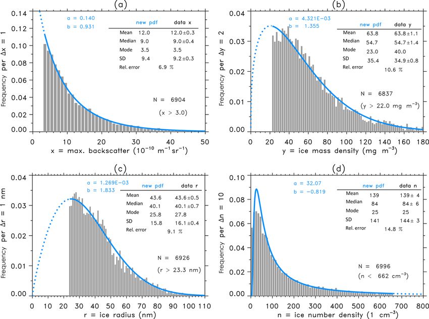
4688                                                                    U. Berger et al.: Probability density distributions of PMC

Figure 1. (a) Logarithm of frequency distribution of maximum backscatter (x = MBS) in units of 10−10 m−1 sr−1 (gray points x > 3; black
circles 0 < x < 3). The bin size is 1x = 1. The straight line (solid red) has been derived from a least-squares fit to MBS data with x > 3.
(b) Same as (a), but original nonlogarithmic frequency distribution (gray bars x > 3; black bars 0 < x < 3). The exponential fit derived from
panel (a) is shown as a red curve. Values of mean, median, and standard deviation are given to compare fit and original data taking into
account a threshold of xth = 3. The relative error given in percent describes the quality of exponential fitting, see text for details.

   We summarize that ice mass density, ice radius, and ice               sion line we estimate d = 0.873. The statistical error for d
number density do not follow an exponential distribution in              is 1d = ±0.012 with a confidence level of 95 %, which indi-
contrast to maximum backscatter. In the following section                cates a significant nonlinearity. Hence we conclude that the
we will show that this is reasonable and is based on the fact            pdf describing the distribution of IMD data is very likely not
that a functional link between MBS and the other data sets of            an exact exponential function and its cumulative distribution
IMD, r and n does miss a linear relationship.                            does not follow precisely a g-function description because
                                                                         the criterion of “linearity” is violated. In Fig. 3b we show a
3.2    Test of linearity between maximum backscatter                     second example for the correlation between MBS and ice ra-
       and ice mass density, ice radius, ice number density              dius n. Again the correlation is about R = 0.55, but now the
       data                                                              power constant is even much smaller with d = 0.497, which
                                                                         is far away from unity. Finally, we investigated the linear-
Linearity between MBS and IMD, ice radius r and ice num-                 ity between MBS and ice number density n where we find a
ber density n data, is a necessary and sufficient condition that         weak negative correlation of R = −0.15 (not shown here). A
also shows that IMD, r and n data, samples are exponen-                  best fit analysis yields a power value of d = −0.534, which
tially distributed, see next section. In the following we will           again fails significantly the constraint of unity. Hence we
test this constraint. Figure 3a shows a scatter plot in a log-           conclude that ice radius and ice number density distributions
arithmic frame for simultaneously measured MBS and IMD                   should also not follow exponential (g-function) distributions.
data. In order to test a linear relationship between x = MBS
and y = IMD we introduce a general fit function described
by a power law condition as                                              4   A new probability density function for PMC
                                                                             parameters
y(x) = cx d ⇔ x(y) = (y/c)1/d                                   (5)
                                                                         In this section we will present the major part of the new sta-
with the two constants c (linear constant) and d (power con-             tistical approach in order to describe frequency distributions
stant). Only for d = 1 we expect a perfect linear dependence             of different PMC parameters.
between x and y. First of all, the logarithmic values of x and              There exists a general mathematical method (“integration
y do not yet have a high linear correlation (R = 0.54), see              by substitution”) that provides the opportunity to transform
Fig. 3a. Since the correlation coefficient R is unequal one, the         between pdfs with different statistical variables. This is done
two regression lines resulting from y(x) : ln x 7 −→ ln y and            by the following procedure: assuming a given pdf P (x) with
x(y) : ln y 7 −→ ln x differ from each other. This means that            variable x, then the transformation from x to a new variable
the best choice of a regression fit is determined by a straight          y(x) with a new pdf Q(y) is specified by
line through the two regression points, which are defined by
the means plus/minus standard deviations of logarithmic x                Q(y) = k∂x/∂yk · P (x(y))                                       (6)
and y data. Note that the positions of regression points also
relate to the half-width of the angle that is spanned by the             with x(y) being the inverse function of y(x). Here the ab-
two regression lines y(x) and x(y). For our mean regres-                 solute value of the derivative ∂x/∂y has to be calculated so

Atmos. Chem. Phys., 19, 4685–4702, 2019                                                    www.atmos-chem-phys.net/19/4685/2019/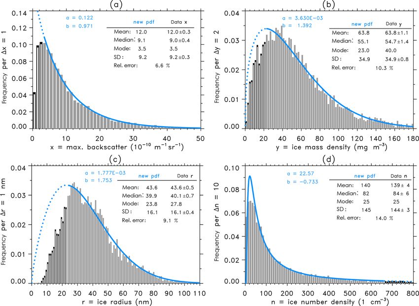
U. Berger et al.: Probability density distributions of PMC                                                                                   4689

Figure 2. (a) Logarithm of frequency distribution of ice mass density (y = IMD) in units of mg m−3 (gray points y > 20; black circles
0 < y < 20). The bin size is 1y = 2. The straight line (solid red) has been derived from a least-squares fit to IMD data with y > 20. (b) Same
as (a), but original nonlogarithmic frequency distribution (gray bars y > 20; black bars 0 < y < 20). The exponential fit derived from (a)
is shown as a red curve. Values of mean, median, and standard deviation are given to compare fit and original data taking into account a
threshold of yth = 20. The relative error given in percent describes the quality of exponential fitting. (c, d) Same, but for ice radius r in units
of nm with bin size 1r = 1 and threshold rth = 20. (e, f) Same, but for ice number density n in units of 1 cm−3 with bin size 1n = 10 and
threshold nth = 30.

that the new pdf Q is defined positively everywhere. In or-                 dence between the two statistical ice variables x and y. In the
der to apply this approach one needs generally two require-                 following we discuss how we satisfy these two requirements.
ments (1) Any transformation between the two pdfs, P and                       We apply this method for two ice parameters, namely
Q, needs an initial guess in one of the two pdfs, either P                  MBS with variable x and an unknown ice parameter named
or Q. (2) An analytic formula of a forward and backward                     u (e.g., this unknown ice parameter might be ice particle ra-
model must be available that describes the functional depen-                dius). For condition (1), we use the hypothesis that the distri-
                                                                            bution of maximum backscatter data (MBS) is perfectly rep-

www.atmos-chem-phys.net/19/4685/2019/                                                          Atmos. Chem. Phys., 19, 4685–4702, 2019
4690                                                                   U. Berger et al.: Probability density distributions of PMC

Figure 3. (a) Maximum backscatter (x = MBS) versus ice mass density (y = IMD) in a logarithmic frame for all data with correlation
coefficient R and regression parameters c and d, see text for more details. Regression points p1/2 = [m ± 1m; n ± 1n] are calculated with
                                               q                                   q
m = 1/N N
          P                    PN                     PN              2 , and 1n = 1/N N (ln y − n)2 . Mean and median are calculated
                                                                                         P
             i ln xi , n = 1/N  i ln yi , 1m =   1/N    i  (ln xi − m)                      i     i
from original nonlogarithmic data. The solid line shows the mean regression defined by regression points and corresponding c and d values.
Dashed lines result from simple regression analysis of y(x) : x ⇒ y and x(y) : x ⇒ y. (b) Same for x = MBS versus ice radius r.

resented by an exponential pdf and its cumulative distribution         with a = e    c)b/d and b = e
                                                                                a (1/e             b/de as
                                                                                       ee

is described by a g function according to Eq. (1). For con-
                                                                                               b
dition (2), we assume a power form of a fit function used in           Z(z) = a|b|zb−1 e−az (a > 0, b 6 = 0).                         (9)
Eq. (5) that also allows us to analytically calculate the inverse
function. We discuss a suitable justification of this assump-          Equation (9) represents our final result. The pdf Z(z) de-
tion in Sect. 6.2. Hence the forward model is u(x) = cx d and          scribes the general form of the new statistical distribution.
the backward model is x(u) = (u/c)1/d . Then the new dis-              Note that the algebraic expressions of Eqs. (8) and (9) for-
tribution U for the arbitrary ice parameter u using Eq. (6) is         mally coincide. This means that any probability distribution
given by                                                               of a new ice parameter that is connected to other ice param-
                                                                      eters through our functional power law (Eq. 5) can be de-
U(u) = k∂x/∂u | · E(x(u))                                     (7)      scribed by the general pdf given by Eq. (9). The constants
           1     u 1/d
                                   1/d                                a and b represent two free parameters in the Z distribution,
      =       ·          · αe−α(u/c) .
          du c                                                         which we name the scale parameter a and the shape param-
                                                                       eter b. Obviously, the Z pdf is identical with an exponential
Equation (7) can be simplified to a more general form with             pdf (or g function) in the limit b = 1. This shows the close in-
                              1/d                                    terconnection of the new Z pdf to the commonly used expo-
                  a ub
             b−1 −e
                     e        1         1
U(u) = e
       a |b|u e
          e  e
                       , e
                         a=α        , e
                                      b= .                     (8)     nential (g-function) approach. We will show in the following
                              c         d                              that any distribution from so different ice parameters, such as
   In a next step we introduce, in an arbitrary manner, a third        maximum backscatter, ice mass density, ice radius, and num-
ice parameter named z for which we assume again the same               ber density of ice particles, can be described on a uniform
power law (Eq. 5) now valid between z and u as                         basis with a high accuracy by Z. Vice versa this indicates
                                                                       that these ice parameters are connected depending on each
z(u) = e
           e
                       c)1/d .
       cud ⇔ u(z) = (z/e
                                 e                                     other by the uniform power law relation (Eq. 5), more details
                                                                       are discussed in Sect. 6.2.
Again we apply Eq. (6) and calculate the unknown pdf Z(z):

Z(z) = k∂u/∂zk · U(u(z))                                               5     Application of the Z distribution to real data
         1  z 1/de
                                  e b−1 −e
                                    e                b/de
                              c)1/d         e a (z/ec)
                                                      e
     =     ·           ae
                      ·eb (z/e                                         5.1    General properties of the Z distribution
        dz e
        e      c
        ab
         e
                          e b
                           e          b/de                            In this section we first show some general characteristics of
                      c)1/d e−ea (z/ec) .
             · z−1 (z/e
        e                              e
     =
         d
         e                                                             the new Z distribution. From these properties we derive con-
                                                                       ditions and constraints that will allow to estimate the specific
At first glance the algebraic expression for Z looks particu-          values of the two free constants in Z, the scale parameter a
larly complex, but Z can be transformed to a general form              and shape parameter b, for a given data sample.

Atmos. Chem. Phys., 19, 4685–4702, 2019                                                  www.atmos-chem-phys.net/19/4685/2019/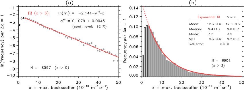
U. Berger et al.: Probability density distributions of PMC                                                                      4691

  First we show that Z is a correct pdf satisfying the nor-        the shape parameter b determines the shape of the Z distri-
                    R∞                                             bution describing nonlinear exponential, exponential, right-
malization condition Zdz = 1:
                         0
                                                                   skewed, left-skewed, or symmetric curves. For 0 < b < 1 the
                                                                   pdf increase is nonlinear and exponentially accelerated to in-
Z∞     Z∞                                      ∞                   finity as z approaches zero. For b = 1 the pdf is exactly an
                     b      |b|   b
  Zdz = a|b|zb−1 e−az dz = − e−az                  = 1.            exponential distribution having a positive finite value for z
                             b                 0
0         0                                                        equal zero. For b > 1, the function tends to zero as z ap-
                                                                   proaches zero. When b is between 1 and 2, the function
The definition range of Z(z; a, b) is z ≥ 0, a > 0, and b 6 = 0    is right-skewed and rises to a peak quickly, then decreases
with Z(z < 0) = 0 and                                              for large z. When b has an approximate value between 3
                     b                                             and 4, the function becomes symmetric and bell-shaped like
Z = a|b|zb−1 e−az ,                                       (10a)    a normal distribution. Note that exact symmetry is given
                                         b                         for a skewness equal to zero, which is true at z = 3.60232.
ln(Z) = ln(a|b|) + (b − 1) · ln(z) − az , b > 0.
                                                                   For b values larger than approximately 5, the function be-
For a negative b the distribution Z is described by                comes again asymmetric changing the skewness to the left.
         |b−1|                                                   For b < 0, the function is skewed to the right and decreases
         1               |b|
                                                                   steeply towards zero as z approaches zero. Note that Z is
Z = a|b|         e−a(1/z) ,                               (10b)
         z                                                         never negative and owns a local maximum described by the
ln(Z) = ln(a|b|) + |b − 1| · ln(1/z) − a(1/z)|b| , b < 0.          mode whenever b is negative or larger than 1. Finally we see
                                                                   that a double-logarithmic presentation of cumulative func-
The cumulative form of Z for b > 0 is given by                     tions describes linear shapes with slope b, see Fig. 4j–l.
                                                                      It is interesting to note that our new Z distribution is
          Z∞                                                       closely related to a more general Weibull distribution (Wilks,
                      b
Zcum (z) = Zdz0 = e−az ,                                  (11a)    1995). Nevertheless there is a difference concerning the
              z                                                    shape parameter b, which in our case is not only defined for
ln(Zcum ) = −azb , ln(| ln(Zcum )|) = ln(a) + b ln(z).             positive values but also for negative values. Such a case is
                                                                   disregarded by a classical 2-D Weibull distribution.
For b < 0 we have to choose the cumulative calculation in             Now we shortly summarize the mathematical descriptions
reverse order starting the integration at zero. Naming the re-     of median, mode, mean, variance, and standard deviation pa-
verse cumulative with index zero as Zcum0   we get                 rameters of Z for the case of a zero threshold. The calcula-
                                                                   tions are described in detail in Appendix B for the general
             Zz                                                    case of a nonzero threshold.
 0                              |b|      b
Zcum (z) =        Zdz0 = e−a(1/z) = e−az ,                (11b)    Median:
              0
                                                                           ln 2 1/b

    0                       0
ln(Zcum ) = −azb , ln(| ln(Zcum )|) = ln(a) + b ln(z).             ν=               .                                        (12a)
                                                                            a
Only the cumulative descriptions from Eqs. (11a) and (11b)         Mode:
allow us, in principle, to roughly estimate the constants a
                                                                         b − 1 1/b

and b for a given data sample using the double-logarithmic
                                                                   η=               for b > 1, b < 0;                           (12b)
functional dependence, whereas the direct logarithm of Z                  ab
(Eqs. 10a, 10b) offers no possibility to solve for a and           η = 0 for 0 < b ≤ 1.
b. However, the method calculating the double-logarithmic
cumulative is not recommended. Several numerical tests             Mean:
showed that a stable estimation of a and b from noisy data
                                                                                b+1
applying this double-logarithmic approach is an almost im-              0        b
possible task. Instead, we propose two different methods that      µ=           1
                                                                                          .                                     (12c)
                                                                            ab
rely on much more powerful principles (see next Sect. 5.2).
Additionally, we have to take care of a possible negative          Variance and standard deviation:
value of b that can be only identified using Eq. (11b). In                                  v
                                                                            b+2               u 0 b+2
                                                                                              u
fact such a case occurs in the analysis of ALOMAR data.                  0 b                         b
                                                                   σ2 =           − µ2 , σ =             − µ2 .
                                                                                              t
In Sect. 5.3 we will give an example where only a negative                   2                       2
                                                                                                                                (12d)
                                                                           ab                       ab
slope parameter describes the distribution of number density
of ice particles.                                                  The expressions of mean and variance use the gamma func-
   Generally, the Z distribution has the ability to characterize              R∞
                                                                   tion 0(t) = x t−1 e−x dx. Notice that the gamma function is
many different types of distributions, see Fig. 4. Especially                         0

www.atmos-chem-phys.net/19/4685/2019/                                                         Atmos. Chem. Phys., 19, 4685–4702, 2019
4692 U. Berger et al.: Probability density distributions of PMC
Figure 4. (a–c) Examples of Z(z) function with different parameter values a and b, see Eq. (10). (d–f) Same but for ln(Z) from Eq. (10);
(g–i) same but for Zcum from Eq. (11); (j–l) same but for ln(| ln(Zcum )|) from Eq. (11).
defined for all real values of t except t = 0 and all negative following equations:
integer values of t. Note also that median, mode, mean, vari- 1/b
ance, and standard deviation parameters of Z coincide with ln 2 b ln 2
ν= + zth −→ a = , (13a)
those of an exponential distribution in the limit as b equals 1. a eb − zthb
m
5.2 Two computational methods to estimate the free
b+1 b
parameters a and b of Z from a given data sample A|b|0 b , azth
µ =− −→ 0 (13b)
ba 1/b
In this section we present two numerical methods to calcu-
b+1
late the scale parameter a and shape parameter b describing = m · ba 1/b + A|b|0 b
, azth .
b
the new Z distribution. First of all, since any measurement
depends on a specific instrumental sensitivity, we have to in- Note that the use of a threshold constraint involves the intro-
troduce a threshold that we name zth . The remaining data duction of a scaling factor A = exp(azth b ), which is present
sample consists of N observations zi with zi > zth . Then we in Eq. (13b). Inserting the algebraic term of a (right side of
calculate the mean m and standard deviation s of data zi us- Eq. 13a into the right side zero-equation Eq. 13b) and using
ing Eq. (3), and also the median value me from data zi . the threshold value of zth yields an equation only for b, which
Method (1): we investigate the corresponding theoretical has to be computed iteratively. Once a numerical value of b
moments from Z. In Appendix B we derive the theoretical has been estimated with a sufficient accuracy, we insert this b
mean µ (Eq. B5) and median ν (Eq. B3) for the Z distri- value into the upper right equation to get the numerical value
bution with a threshold constraint. Taking the estimates of for a.
mean m and median m e from the sample as best proxies for We note that in classical statistics the method of moments
the theoretical mean µ and median ν values of Z, we get the determines a and b from the mean and variance equations.
Atmos. Chem. Phys., 19, 4685–4702, 2019 www.atmos-chem-phys.net/19/4685/2019/U. Berger et al.: Probability density distributions of PMC 4693
In principle this approach should be possible here too, but in the preservation of mean and median values. Nevertheless
practise the algebraic structure of the variance equation is too standard deviation and mode also always show a good agree-
complicated, see Eq. (B6) in Appendix B. This means that ment within the error range. A closer look to the maximum
the variance equation, if at all, is only iteratively solvable, backscatter distribution shows that MBS data are almost per-
whereas the use of the median equation offers an analytical fectly exponentially distributed with b = 0.931, which is not
transformation to a. Generally, we recommend to apply the too far away from b = 1 for an exact exponential pdf. As
proposed method using the mean and median equations. This we had already shown, see Sect. 3.1.1, MBS data are very
straight-forward method is easy to program and produces re- likely exponentially distributed, now the Z-distribution anal-
liable estimates of parameters a and b. ysis confirms this result. Hence we conclude that the com-
Method (2): we also present a second method using a max- monly used exponential (g-function) analysis might only be
imum likelihood approach, see Appendix C. The parameters a reasonable statistical method in the case of analyzing MBS
are again calculated from two equations (Eq. C5) with lidar data.
P b In contrast to MBS, the Z distribution of IMD shows a
1 b zi
= −zth + , (14) function that converges rapidly to zero for small IMD values.
a N The distribution is described with b = 1.355, which signifi-
ln zi · zib
P P
1 b ln zi cantly deviates from b = 1 for a precise exponential function.
0 = + a · ln zth · zth + −a· .
b N N Note that the mode of the data sample at 40 mg m−3 differs
Interestingly, the left equation includes a term 1/N zib ,
P from the theoretical mode of 23 mg m−3 because of a rela-
which is the mean of the sample values weighted byP power b, tively high statistical noise in the data. But mean, median,
whereas the right equationP includes the mean 1/N ln zi of and standard deviation values agree almost perfectly. Simi-
logarithmic data and 1/N zib ln zi . This shows a similarity lar to IMD, the ice radius distribution indicates a significant
to the computation of regression points used in Fig. 3. We nonexponential behavior with b = 1.833. The distribution
insert a into the right equation that yields a unique equation converges to zero as the radius approaches zero. The curve
for b, which again can be solved iteratively. Once b is fixed, is skewed to the right and has a maximum at r = 25.8 nm,
the left equation allows us to determine a. In the following which differs only slightly from the mode of the data sample
we will test our lidar data samples with these two procedures at r = 27.8 nm. Again mean, median, and standard deviation
and we will show that both methods produce almost identical values agree almost perfectly.
results. The sample of ice number density shows a completely dif-
ferent behavior with a slope parameter that is negative with
5.3 Z distributions applied to ALOMAR data b = −0.819. The physical meaning is that the parameter ice
number density is negatively correlated with all other ice pa-
Applications of the Z distribution to ALOMAR data of max- rameters. For example, large ice numbers n correspond to
imum backscatter (x), ice mass density (y), ice particle ra- small ice radii, IMD and MBS values. As a consequence this
dius (r), and ice number density (n) are shown in Fig. 5. leads to a threshold of n in the reverse direction, that is from
Note that thresholds have been computed from the regres- large values to small values defined by n < nth = 662 cm−3 .
sion functions (Eq. 5) described in Sect. 3.2 on the basis One can see this feature in the right tail of Z(n) plotted as
of xth = 3 × 10⁻¹⁰ m−1 sr−1 , resulting in yth = 22 mg m−3 , a dashed curve, see Fig. 5d. The reverse behavior is also
rth = 22.3 nm, and nth = 662 cm−3 . The values of scale pa- present for small values of n. Small values of n are measured
rameter a and shape parameter b have been calculated with for very bright PMC events with large MBS that have small
the method of mean and median equations (method 1). occurrence rates. Therefore, the number of small ice parti-
Then the theoretical curves of Z and theoretical values of cles has a relatively high uncertainty due to their low occur-
mean, median, mode, and standard deviation have been cal- rence frequency, and it is this statistical error that produces
culated by inserting the values of a, b, and threshold zth into some deviations from the fit curve to the data in the range
Eqs. (B1)–(B6). Obviously the pdf Z sometimes has no sim- of n = 0–80 cm−3 . We note that the numerical procedure
ple exponential shape, which is the case for ice mass density, computing the pair (a, b) from the method of mean/median
ice radius, and ice number density. As we see in Fig. 5 all Z- (Eqs. 13a, 10b) has automatically detected the existence of a
pdf curves (in blue) match the original data histograms with a negative slope parameter b without any a priori information.
high accuracy. The relative error is in a range of about 6 %– Now we repeat the analysis using method 2. Figure 6 sum-
10 % except that ice number density has a relative error of marizes the (a, b) values and statistical moments calculated
15 %. When we compare the mean, median, mode, and stan- from the method of maximum likelihood estimators. As can
dard deviation derived from the theoretical distribution and be seen the maximum likelihood approach computes almost
corresponding estimates from data samples, we see a precise identical results for all ice parameters. We have also added
coincidence of mean and median values. Not surprising this in Fig. 6a–c the histogram bars (in black) for all data be-
is due to the fact that the parameters a and b have been com- ing smaller than the threshold. Please keep in mind that the
puted by the mean and median method, which guarantees calculation of theoretical distribution curves is based exclu-
www.atmos-chem-phys.net/19/4685/2019/ Atmos. Chem. Phys., 19, 4685–4702, 20194694 U. Berger et al.: Probability density distributions of PMC
Figure 5. Frequency distributions and Z-function analysis of ALOMAR data. Parameters a and b have been estimated with the mean and
median methods. The relative error given in percent describes the quality of the Z-function fit; (a) maximum backscatter data x. (b) ice mass
density y; (c) ice particle radius r; (d) ice number density n, see text for more details.
sively on data larger than the threshold. Hence, decreasing tificial unknown data samples of various ice parameters that
or increasing a threshold will change the specific values of approximate true data to a high degree. We think that such
a and b. Figure 6d shows the ice number density distribu- an application is one of the most beneficial outcomes from
tion where we have added in the histogram (in black) all data the new Z-distribution approach. We explain the numerical
being larger than the threshold. Again, also the maximum procedure by the help of a practical example.
likelihood method has automatically detected the existence We already showed a linear dependance in the logarithmic
of a negative slope parameter b for the ice number density frame using linear regression (LR) for maximum backscatter
distribution. and ice particle radius, see Fig. 3b. Hence we can compute ar-
tificial ice radius proxies e
ri , named as LR proxy of true data
ri , as a function of MBS-data xi from the regression power
6 Discussion law function (Eq. 5) with e ri = cxid and with power law coef-
ficients c = 13.509 and d = 0.497. Figure 7a shows a com-
6.1 Construction of artificial data parison between LR proxy and original ice radius data where
we test the identity of the two data samples. The correlation
In the derivation of the Z distribution we used the as- coefficient is the same as shown in Fig. 3b with R = 0.55.
sumption that all ice parameters of maximum backscatter Mean and median values of proxy and original data are al-
x = MBS, ice mass density y = IMD, ice particle radius r, most identical, and a regression analysis shows a perfect
and ice number density n are connected with one another by identity (c = 1.000 and d = 1.000). Now we calculate the
the power law given in Eq. (5). In Sect. 5.3 we showed that frequency histogram of LR proxy ice radii, see Fig. 7b, and
the Z pdf describes with a high accuracy each distribution of compare the histogram with the original Z distribution of ice
these ice parameters, which, in turn, means that indeed there radii already shown in Fig. 5c. We find that the LR proxy ap-
exists at least an approximative power law between ice pa- proximates the mean, median, mode, and standard deviation
rameters. We discuss a suitable justification of this power law values of the original Z distribution with an relative error of
relation in more detail in Sect. 6.2. In the following we will 9.5 % comparable to the original error of 9.1 %. We conclude
show that the use of a Z distribution allows us to construct ar-
Atmos. Chem. Phys., 19, 4685–4702, 2019 www.atmos-chem-phys.net/19/4685/2019/U. Berger et al.: Probability density distributions of PMC 4695
Figure 6. Same as Fig. 5, but parameters a and b have been estimated from the maximum likelihood method. (a–c) Maximum backscatter,
ice mass density, and ice radius: gray bars indicate values larger than the threshold and black bars indicate values smaller than the threshold.
(d) Ice number density: gray bars indicate values smaller than the threshold and black bars indicate values larger than the threshold.
that a linear regression analysis of logarithmic data offers a (i = 1, . . ., N ) into the z domain with xi 7 −→ zi : z = ax xibx
good opportunity to approximate data, provided that a pair of followed by a second transformation with zi 7 −→ ri : ri =
data samples exists that allows for the calculation of power (zi /ar )1/br resulting in
law coefficients c and d from regression methods. " #1/br
Now the Z-distribution approach offers a more gen- ax · xibx
eral possibility to derive artificial data samples without any xi 7 −→ zi 7 −→ ri : ri = = c · xid (15)
ar
knowledge of correlation and regression coefficients. Indeed
we will show that results from the Z approach are very close with
to results from a regression analysis. Again, our goal is to ap-
proximate ice radius data from a given maximum backscat- 1/br
ax bx
ter data sample. But now we suppose that no data of ice c= , d= .
ar br
particle radii r exist, hence any correlation and regression
analysis is not possible. First, we assume that a data sam- Note that the derivation of c and d in Eq. (15) is based on
ple of x = MBS of number N exists and also its Z distri- the same mathematical steps when we developed the Z dis-
bution Z(x, ax , bx ) with ax = 0.140 and bx = 0.931 is well tribution from Eqs. (8) to (9). Inserting the ax , bx , ar , and br
known, see Fig. 5a. Secondly, we assume that we know a values into Eq. (15) determines the power law coefficients for
priori the form of the Z distribution Z(r, ar , br ) of ice ra- Z proxy e r with c = 12.994 and d = 0.508. These values do
dius r, e.g., with values of parameters ar and br from Fig. 5c not exactly coincide with c and d values obtained from the
(ar = 1.269 × 10⁻³ , br = 1.833). Please keep in mind that regression method, see above, but the identity test between Z
such information about scale and shape parameters of the ice proxies and true ice radii shows a very good coincidence, see
radius distribution could be also provided from independent Fig. 7c. Again, mean and median values of proxy and orig-
satellite measurements that are capable of measuring ice par- inal data are practically identical, and a regression analysis
ticle radii, e.g., AIM-SOFIE. shows an almost perfect identity (c = 1.095 and d = 0.980).
Our new proxy method (Z proxy) requires the fol- Finally we calculate a frequency histogram of Z proxies, see
lowing transformations. We first transform the xi values Fig. 7d, and find a good agreement between proxies and true
www.atmos-chem-phys.net/19/4685/2019/ Atmos. Chem. Phys., 19, 4685–4702, 20194696 U. Berger et al.: Probability density distributions of PMC
Figure 7. (a) Proxy p of ice radius versus original ice radius data without any threshold. The proxy has been derived from maximum
backscatter data using the fit function that has been estimated by linear regression (LR proxy) between original logarithmic MBS and ice
radius data, see Fig. 3b. (b) Frequency distribution of LR proxy (gray and black histogram) with a threshold rth = 23.3 nm. For comparison
we also plot the original Z-pdf curve (blue) from the analysis of original ice radius data, see Fig. 5c. The relative error describes the accuracy
between LR-proxy data and original Z-function fit. (c) Same as (a), but for Z-proxy data resulting from the Z-pdf analysis of MBS data,
see text for more details; (d) same as b with Z-proxy data.
pdf. Mean, median, and standard deviations of Z-proxy data IWC observed by the satellite. We think that our proposed
correspond perfectly to original ice radius data, and the rela- transformation method could be very helpful to connect dif-
tive error has now even decreased to 9.2 %. ferent ice parameter data from different instruments, either
We summarize that we present a new method in order from satellite observations or ground-based measurements.
to construct artificial data samples provided Z-descriptions We also think that this new approach might be important in
of these data sets exist. By means of a consecutive arrang- trend analysis of PMC.
ing of ice parameters starting at a given data sample, this In the next section we will discuss the power law assump-
method allows us to construct any artificial data sample tion (Eq. 5) and the physical meaning of the shape parameter
within (x, y, r, n). This method can also be applied to other b, which might be introduced as a new trend variable in the
data sets, e.g., ice parameter measurements from satellite ob- analysis of PMC long-term changes.
servations. For example, a data sample of ice water content
(IWC) obtained from satellite measurements might be ana-
lyzed in terms of a Z distribution estimating the scale and 6.2 Discussion of the power law assumption between
shape parameters a and b of the IWC distribution. This would PMC parameters
allow us to establish a connection between satellite IWC
data to lidar data samples (x, y, r, n) through Eq. (15), hence
the satellite IWC data could be transferred to lidar maxi- In this section we discuss some theoretical aspects of the
mum backscatter, ice mass density, ice particle radius, and power law dependence on ice parameters in order to validate
ice number density. Vice versa the knowledge of a satellite the justification of Eq. (5). We use again the assumption as
IWC Z distribution would allow us to transform lidar obser- already discussed in Sect. 2 that at the altitude of maximum
vations into IWC proxies and compare these with the original brightness (MBS) and ice mass density (IMD) there exists in
the real atmospheric background an ice particle distribution
Atmos. Chem. Phys., 19, 4685–4702, 2019 www.atmos-chem-phys.net/19/4685/2019/U. Berger et al.: Probability density distributions of PMC 4697
√ Rx
that is perfectly Gaussian-distributed (Ni ) as 2/ π 0 exp(−t 2 )dt is part of the solution:
4 37 3 5 (τ − ri )
xi = π ρice n ri erf √
! 3 50 8ri
1 τ − ri 2
1 √
Ni (τ ) = √ exp − . 2
σi 2π 2 σi − √ ri 25τ 2 + 25ri τ + 33ri2
125 π
!#∞
25τ 25 τ 2 + ri2
We also assume that the geometric shapes of these ice par- exp − .
4ri 8ri2
ticles are spheres with ice radii τ with mean radius ri and 0
variance σi2 . Again index i = 1, . . ., N relates to the ith mea- The integral for xi includes the term τ 5.8 that arises from
surement inR a given data sample of number N . Ni is nor- Mie-scatter theory for light scattering of a wavelength of
∞
malized to 0 Ni (τ )dτ = 1. When we assume an ice num- 532 nm (ALOMAR RMR lidar) at spheres in a range of radii
ber densityRof ni particles per cubic centimeter we get the with 1–100 nm. The exponential value of 5.8 approximates
∞
expression 0 ni · Ni (τ )dτ = ni . Note that mean ice radii ri exact Mie-scatter calculations with a relative error less than
and ice number densities ni are elements of our lidar data 0.5 % in this radii range. Unfortunately, the integral can only
climatology, which we have introduced in Sect. 2. be solved analytically if the exponent is an integer number
Furthermore, we assume from the analysis of lidar ob- as 5 or 6. Nevertheless, we are able to solve this integral by
servations (three-color measurements) that the relation of means of numerical methods with the specific exponent of
mean radius and variance is according to σi = 0.4 ri for 5.8. In a next step, we construct analytical approximations
ri < 37.5 nm and σi = 15 nm for ri ≥ 37.5 nm (Baumgarten fx (ri ) and fy (ri ) for both integral solutions using a typical
et al., 2010). This assumption has also been applied in the value of n = 200 cm−3 with
analysis of AIM/SOFIE-CIPS PMC satellite data (Lumpe
et al., 2013; Hervig and Stevens, 2014). In order to sim- fx (ri ) = xi = a1 aL nri5.8 ,
plify calculations we apply this relation σi = 0.4 ri also for 4
ri larger than 37.5 nm. We now investigate the question of fy (ri ) = yi = a2 π ρice nri3 .
3
which backscatter lidar and ice mass signals result from such The linear constants a1 and a2 with values a1 = 4.20 and
an ice distribution. a2 = 1.47 are optimal dimensionless parameters. fy approx-
We compute the mass of a spherical ice particle with ra- imates the analytical solution of yi with a relative error less
dius τ as 4/3π ρice τ 3 with density of ice ρice = 932 kg m− 3. than 0.7 % in the range ri = [0, 45 nm], and less than 1.2 %
The backscatter signal from a single ice particle is calculated in the range ri = [45, 70 nm]. A precise solution of xi re-
as aL τ 5.8 with the lidar constant aL = 1.5 × 10⁻¹¹ m2 . Then sulting from numerical methods of integration is approxi-
the maximum backscatter xi and ice mass density yi are es- mated by fx with a relative error less than 0.3 % in the range
timated by an integration of the radius distribution from zero ri = [0, 45 nm], then the relative error increases linearly to a
to infinity as maximum error of 5 % at ri = 70 nm. We find that the solu-
tions fx and fy approximate the general power law condi-
tion p = cq d (Eq. 5) inside a small error range. Hence these
Z∞
analytical examples show that MBS is a function of ice ra-
xi = aL n τ 5.8 Ni (τ )dτ dius proportional to ∼ r 5.8 (d = 5.8), the same is also true
0 for IMD (∼ r 3 , d = 3). It also follows that MBS and IMD
Z∞ ! are consequently connected through a power law condition
1 τ − ri 2
1
= aL n τ 5.8 √ exp − dτ with MBS ∼ IMD5.8/3 (d = 5.8/3 = 1.93).
0.4 ri 2π 2 0.4 ri But the new form of the Z-distribution technique opens
0
Z∞ up whole new perspectives for the validation of the analyti-
4 cal examples based on the ALOMAR lidar data samples. We
yi = π ρice n τ 3 Ni (τ )dτ
3 transform the z distribution of IMD into the MBS domain us-
b
0 ing Eq. (15) with yi 7 −→ zi : zi = ay yi y and zi 7 −→ xi : xi =
Z∞ ! (zi /ax )1/b x that gives
1 τ − ri 2
4 3 1
= π ρice n τ √ exp − dτ " #1/bx
3 0.4 ri 2π 2 0.4ri a y · y by
0 x= = c · yd (16)
ax
assuming a constant number density n of ice particles. Only with
1/bx
the integral of yi is analytically computable with a solution ay by
in which the error function defined by the integral erf(x) = c= , d= .
ax bx
www.atmos-chem-phys.net/19/4685/2019/ Atmos. Chem. Phys., 19, 4685–4702, 20194698 U. Berger et al.: Probability density distributions of PMC
We insert into Eq. (16) the values of ax = 0.140, bx = 0.931, We introduce a new probability density distribution
ay = 4.321 × 10⁻³ , and by = 1.355 from Fig. 5a and b and (Z function, see Eq. 9) that instead assumes a general power
get c = 0.023 and d = 1.46. The power constant (d = 1.46) law relation among ice parameters, see Eq. (5). The new
derived from the shape parameters bx and by of the Z- Z distribution is described by two free constants with scale
distribution analysis of real ALOMAR IBS and IMD data parameter a and the shape parameter b. We point out that the
is significantly different from the power estimate (d = 1.93) new distribution is closely related to a more general Weibull
belonging to the analytical example that necessitates vari- distribution. The new distribution has been applied to maxi-
ous assumptions, e.g., Gaussian-distributed ice particles at mum backscatter, ice mass density, ice radius, and ice num-
the height of maximum backscatter, constant ice particle ber density data from the ALOMAR data set. As a result all
number, or spherical shape of ice particles. Hence, we con- data distributions are described with a high accuracy by Z.
clude that the determination of shape parameters b from a Z- We discuss that the exponential distribution (g function) is a
distribution analysis of observational data therefore provides special case of the more general Z function with shape pa-
a qualitative indication of the actual microphysical state that rameter b = 1. We present two numerically stable methods
controls real ice formation processes. This leads to the idea (method of mean and median, method of maximum likeli-
that as a future task long-term changes in PMC formation ness) that allow to derive the values of free constants a and b
might be characterized by potential long-term changes in b describing the actual Z-function shape for a given data sam-
that indicate long-term changes in atmospheric background ple.
conditions and microphysical ice constraints of ice forma- Perhaps the most important application of the new method
tion. is the possibility to construct unknown data sets for different
ice parameters that approximate true data to a high degree.
We show in Sect. 6.1 that a linear regression analysis in a
7 Summary and conclusions logarithmic data frame offers a good opportunity to approx-
imate data provided that a pair of data samples exists that
In this study we present a new method to describe statisti-
allows for the calculation of power law coefficients c and d
cal probability density functions (pdfs) for different ice pa-
from regression methods. The Z-distribution approach offers
rameters of PMC. We analyze a climatology of ice seasons
a more general possibility to derive artificial data samples
from 2002 until 2016 as measured by the ALOMAR lidar.
without any knowledge of correlation and regression coeffi-
From this data set we derive ice cloud parameters of maxi-
cients. This allows for the connection of different observa-
mum backscatter, ice mass density, ice radius, and ice num-
tional PMC distributions of lidar and satellite data, and also
ber density whose occurrence frequencies are investigated
with distributions resulting from ice model studies. In par-
with respect to exponential distributions. We show that only
ticular, the statistical distributions of different measured ice
maximum backscatter follows an exponential distribution,
parameters can be compared with each other on the basis of
whereas ice mass density, ice radius, and ice number den-
a common assessment that again should be helpful in com-
sity frequencies fail to fit satisfactorily to an exponential dis-
bining trend analysis of PMC long-term time series from dif-
tribution. The reason for these deviations from exponential
ferent observational data sets.
behavior is based on the fact that these ice parameters are not
linearly dependent on each other.
Data availability. The ALOMAR lidar data are available at:
ftp://ftp.iap-kborn.de/data-in-publications/BergerACP2019/
(Baumgarten, 2019).
Atmos. Chem. Phys., 19, 4685–4702, 2019 www.atmos-chem-phys.net/19/4685/2019/U. Berger et al.: Probability density distributions of PMC 4699
Appendix A: Properties of the exponential distribution Appendix B: Properties of Z distribution
(g function)
In the following all quantities take into account a threshold
When considering a thresholdR(xth ) the exponential pdf E(x) b ). Setting the
zth . We introduce a scaling factor A = exp(azth
∞
is normalized according to A xth E(x)dx = 1 with a scaling threshold to zero means a scaling factor A = 1 and gives the
factor A = exp(αxth ). It follows that the mean µ is then given regular expressions for cumulative pdf, median, mode, mean,
by and variance, see Eqs. (12a)–(12d).
Probability density function Z(z ≥ zth , a > 0, b 6= 0):
Z∞
µ= x · AE(x)dx 0 Z(z) = A · a|b|zb−1 e−az ,
b
(B1)
xth Z∞
b b
Z∞ 1 = eazth · a|b|zb−1 e−az dz.
=A x · αe−αx dx 0 zth
xth
∞ Cumulative form of Zcum :
(αx + 1) e−αx
= −A
α xth Z∞
b
(αxth + 1) e−αxth Zcum (z) =A a|b|zb−1 e−az dz (B2)
= 0 − (−)eαxth .
α z
b ∞ b
This yields for the mean = −Ae−az = A · e−az , z ≥ zth .
z
µ = xth + 1/α. (A1) Median ν:
The median ν denotes the boundary of separating the higher Z∞ Z∞
b
half from the lower half of the distribution with 0.5 = Zdz = Aa|b|zb−1 e−az dz
Z∞ Z∞ ν ν
∞ ∞
0.5 = A · E(x)dx = A α exp(−αx)dx 0 = −Ae−αx
0
ν = −Ae −aν b
= Ae−aν
b
ν
ν ν
=0 − (−)eαxth · e−αν .
1/b
ln(2A)
The equation is solved for the median with −→ ν = (B3)
a
b
!1/b
ν = xth + ln(2)/α. (A2) ln 2 + ln(eazth )
=
The mode is the value η at which AE(x) takes its maximum a
value
ln 2
1/b
b
= + zth .
η = xth . (A3) a
The variance σ 2 in an exponential distribution considering a Mode η:
threshold is calculated with ∂Z b
=0 = −A · a|b|zb−2 abzb − b + 1 e−az (B4)
Z∞ Z∞ ∂z
σ2 = (x − µ)2 · AE(x) dx 0 = A (x − µ)2 · αe−αx dx 0 b − 1 1/b
−→ η = (b > 1, b < 0).
xth xth ab
∞
A (α (x − µ) (α (x − µ) + 2) + 2) e−αx
=− Mean µ:
α2 xth
(α (xth − µ) (α (xth − µ) + 2) + 2) e −αxth Z∞ Z∞
=0 − (−)eαxth . µ= zZdz = A a|b|zb e−az dz
b
(B5)
α2
zth zth
Inserting µ = xth + 1/α simplifies the algebraic expression
b+1 b
and shows that the variance σ 2 (standard deviation σ ) is in- A|b|0 b , azth
dependently from a given threshold: =− 1
.
ba b
σ 2 = 1/α 2 . (A4)
www.atmos-chem-phys.net/19/4685/2019/ Atmos. Chem. Phys., 19, 4685–4702, 2019You can also read