Beginner's Guide to GOES-R Series Data - How to acquire, analyze, and visualize GOES-R Series data

Version 1.1

Beginner’s Guide to
GOES-R Series Data
How to acquire, analyze, and visualize GOES-R Series data

Resources compiled by Danielle Losos, GOES-R Product Readiness and
Operations
Last Updated on February 8, 2021

Document Change Record

Version
 ersion Date Slides Affected Description

1.0 10/21/2020 All Initial

1.1 2/8/2021 8, 12, 15-17, 19-21, The following content was added: additional GOES-R
 24, 26-29 imagery viewing platforms; AWS “S3 Explorer” user
 interface for file browsing; Geo2Grid software; Python
 packages (satpy, GOES-2-Go, goespy); section on GIS
 processing (converting netCDF files to GeoTIFFs,
 transforming data to shapefiles).

 2

Contents
Part
 art 1: The GOES-R Series ● Visualize with Python: Custom Packages 21
 ● Introduction to the GOES-R Series 5 ● Visualize with Earth Engine 22
 ● GOES-R Series Instruments 6 ● Technique: Radiance to Reflectance 23
 ● Advanced Baseline Imager (ABI) 7 ● Technique: Generating Composites 24
 ● Mesoscale Domains 8
 ● GOES-R Data Products 9 Part 4: How Can I Process the Data Using GIS?
 ● Product Maturity and Data Availability 10 ● Make GOES-R Series Data GIS-compatible 26
 ● Convert NetCDF files to GeoTIFFs 27
Part 2: Where Can I Access the Data? ● Transform Discrete Data to Shapefiles 28
 ● View GOES-R Imagery 12 ● Transform Continuous Data to Shapefiles 29
 ● View GOES-R Imagery with AWIPS 13
 ● Access Data Files: NOAA CLASS 14 Part 5: Frequently Asked Questions
 ● Access Data Files: Amazon, Microsoft, OCC 15 ● How are GOES-R Series files formatted? 31
 ● Access Data Files: Google Cloud 16 ● How do I pre-process GOES-R Series data? 32
 ● Use Python to Retrieve Data from AWS 17 ● How are AB1 L1b products georeferenced? 33
 ● Why is data not available on a given date? 34
Part 3: How Can I Display the Data? ● Other Questions and Contact 35
 ● Visualize with Command Line: Geo2Grid 19
 ● Visualize with Python: Basics 20 Appendix A: Acronym List 36

 3

Part 1.

 The GOES-R Series

 4

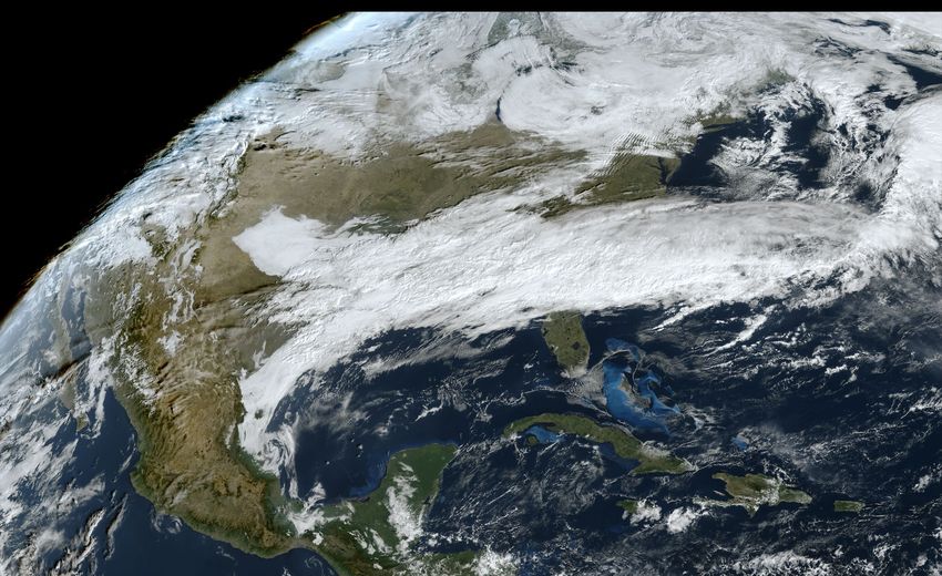
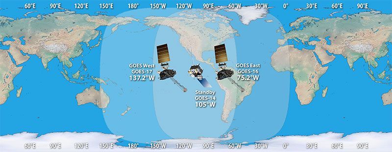
Introduction to the GOES-R Series
 ● Geostationary Operational Environmental Satellites (GOES) are developed, launched and operated in a
 collaborative effort by NOAA and NASA, and have been in operation since 1975.
 ● The latest generation of geostationary satellites, with its first launch in 2016, is the GOES-R Series.
 ● The GOES-R Series is a four satellite program, which maintains two operational satellites at all times, as
 well as third standby satellite in “storage mode” on-orbit as a ready spare (currently GOES-14).
 ○ GOES-R (GOES-16, GOES East) launched in November 2016, replacing GOES-13. It orbits at 75.2⁰ W longitude, with
 coverage of North and South America and the Atlantic Ocean to the west coast of Africa
 ○ GOES-S (GOES-17, GOES West) launched in March, 2018, replacing GOES-15. It orbits at 137.2⁰ W, with coverage of
 western North America and the Pacific Ocean
 ○ GOES-T and GOES-U, currently scheduled for launch in 2021 and
 2024 respectively, will assume operational roles as GOES-16/17 are
 retired.
 ● The GOES-R satellites have six different instruments onboard. See
 Slide 6 for descriptions of each instrument.
Useful links for background information:
 ● Mission Overview, GOES History, GOES-R Data Book (technical
 overview of satellite and ground systems)
 Figure 1. The geographic ranges of GOES-16 and 17
 together cover the North American continent. 5

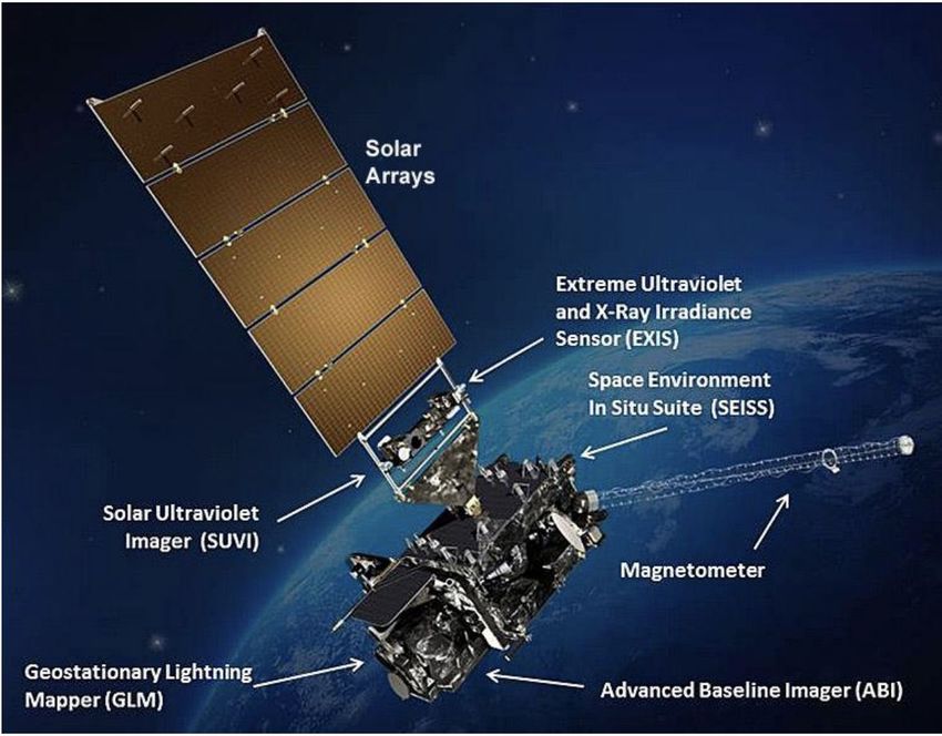
GOES-R Series Instruments
Earth-pointing:
 ● Advanced Baseline Imager (ABI) - the primary instrument for imaging Earth’s
 weather, oceans and environment. See Slide 7 for more details.
 ● Geostationary Lightning Mapper (GLM) - a single-channel, near-infrared
 optical transient detector that can identify momentary changes in an optical
 scene, indicating the presence of lightning.
Sun-pointing:
 ● Extreme Ultraviolet and X-ray Irradiance Sensors (EXIS) - monitors solar
 irradiance in the upper atmosphere using two primary sensors: the Extreme
 Ultraviolet Sensor (EUVS) and the X-Ray Sensor (XRS).
 ● Solar Ultraviolet Imager (SUVI) - a telescope that monitors the sun in the
 extreme ultraviolet wavelength range, detecting solar flares and solar
 Figure 2. GOES-R Series satellites are composed of 6
 eruptions, and compiling full disk solar images. instruments, and powered by a solar panel array.
In-situ:
 ● Magnetometer (MAG) - measures the space environment magnetic field that controls charged particle dynamics in the outer
 region of the magnetosphere.
 ● Space Environment In-Situ Suite (SEISS) - monitors proton, electron, and heavy ion fluxes in the magnetosphere using four
 sensors: the Energetic Heavy Ion Sensor (EHIS), the High and Low Magnetospheric Particle Sensors (MPS-HI and MPS-LO), and
 the Solar and Galactic Proton Sensor (SGPS). 6

Advanced Baseline Imager (ABI)
● ABI is a multi-channel passive imaging radiometer that images Earth’s weather, oceans and
 environment with 16 spectral bands (2 visible, 4 near-infrared, and 10 infrared channels).
 ○ ABI Bands Technical Summary Chart
● Spatial resolution is 0.5, 1, or 2 km, depending on the band (see above-linked chart).
● Geographic coverage
 ○ Full Disk: a circular image depicting nearly full coverage of the Western hemisphere (GOES-16 / GOES-17).
 ○ CONUS/PACUS : a 3,000 (lat) by 5,000 (lon) km rectangular image depicting the Continental US (CONUS)
 (GOES-16) or the Pacific Ocean including Hawaii (PACUS) (GOES-17).
 ○ Mesoscale: a 1,000 by 1,000 km rectangular image. GOES-16 and 17 both alternate between two different
 mesoscale geographic regions (domains). See Slide 8 for a complete description of mesoscale domains.
● ABI has multiple scan modes.
 ○ Mode 4 - A contingency mode. Produces a full disk image every 5 minutes.
 ○ Mode 3 - The cooling timeline mode used by GOES-17 during four time periods per year. This operation
 mitigates the number of saturated images resulting from the loop heat pipe (LHP) temperature regulation
 anomaly. Mode 3 produces a full disk image every 15 minutes, and images of both mesoscale domains every 2
 minutes.
 ○ Mode 6 - The default operational mode for GOES-East & West. Produces a full disk every 10 minutes, a
 CONUS/PACUS image every 5 minutes, and images from both mesoscale domains every 60 seconds.
 7

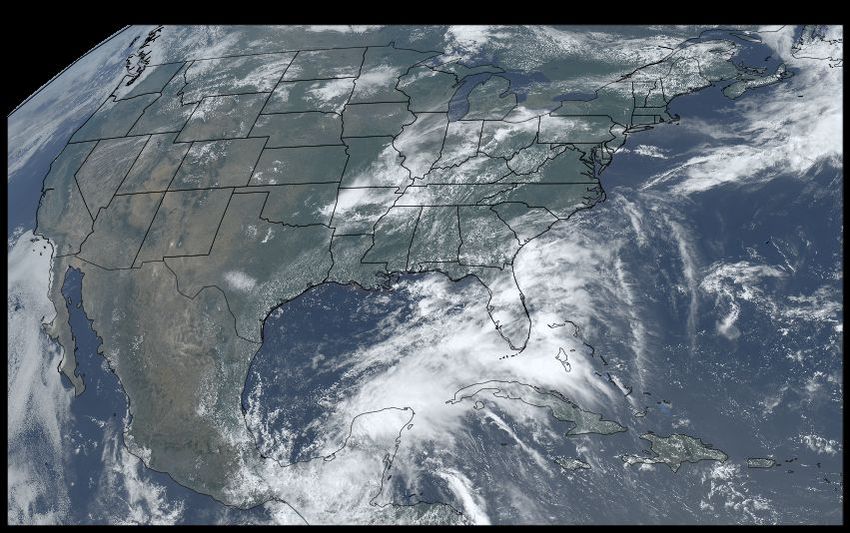
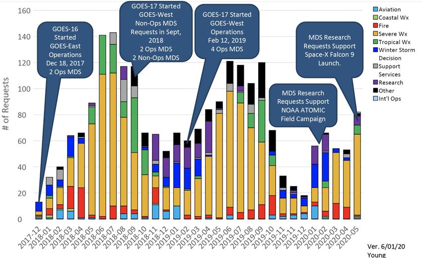
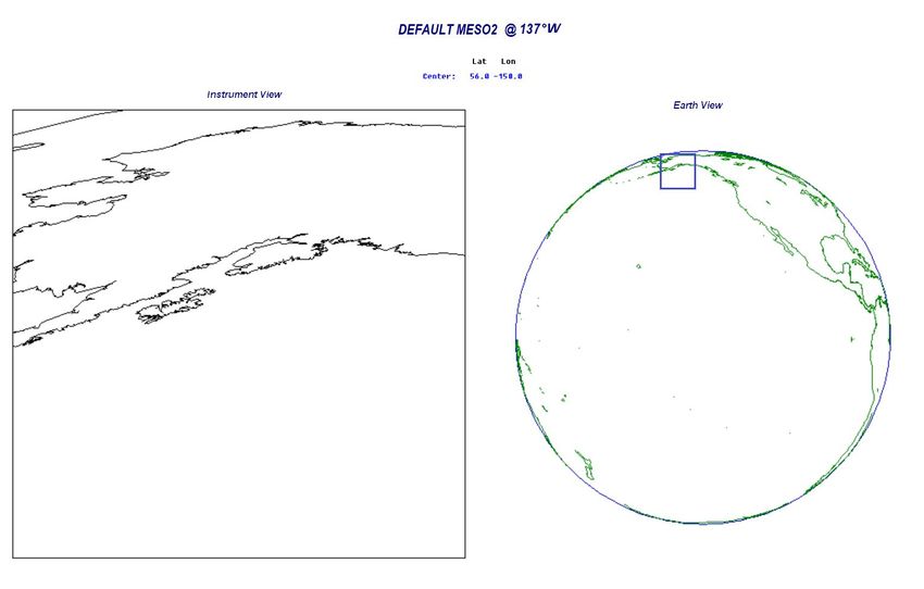
Mesoscale Domains Number of Mesoscale Requests by Month

 ● Mesoscale domains are 1,000 by 1,000 km movable
 rectangular regions. Mesoscale scans frequently revisit an area
 of interest to monitor regional conditions.
 ● GOES-16 and 17 each have two default domains (see below),
 however the domains can be positioned anywhere within the
 full disk upon request. Requests are placed by National
 Weather Service (NWS) Weather Forecast Offices (WFOs).
 ○ See the graph (right) of mesoscale requests by month.
 ○ Check out the live feed of current mesoscale locations.
 ● In Mode 6, the ABI on both GOES-16 and 17 scans either the
 same mesoscale domain every 30 seconds, or two separate
 Figure 3. The frequency of mesoscale domain requests varies
 mesoscale domains every 60 seconds. overtime, peaking during summer months.

Figure 4a. Figure 4b.
The GOES-16 The GOES-17
default default
mesoscale mesoscale
scan sectors scan sectors
are the East are the West
Coast and Coast and
Midwest. MESO 1 (East Coast) MESO 2 (Midwest) Alaska. MESO 1 (West Coast) MESO 2 (Alaska) 8

GOES-R Data Products
● To visualize GOES-R data, select one of many available products.
 ○ Here is a list of all the GOES-R products made available to the user community by NOAA.
● Level 0 (L0):
 ○ L0 products are observation data received directly from the 6 satellite instruments. The data is not meaningful
 to most users prior to processing by the ground system.
● Level 1b (L1b):
 ○ L1b products are calibrated and, where applicable, geographically corrected, L0 data. This means that the data
 has been processed so that its values are in standard units of physical quantities.
 ○ For ABI, the L1b product is Radiances. This is useful for users who require radiance units, instead of
 reflectance/brightness (Kelvin) units.
 ○ All of the instruments have L1b products available except GLM, which is only distributed as an L2+ product.
 ○ For technical information, see the Product User Guide (PUG) Volume 3: L1b Products, Revision 2.2.
● Level 2+ Products:
 ○ L2+ products contain environmental physical qualities, such as cloud top height or land surface temperature.
 Aside from the GLM Lightning Detection Product, the data source for these products is the ABI L1b data
 ○ The mission-critical ABI product is Cloud and Moisture Imagery (CMI), which utilizes all 16 ABI spectral bands,
 and is used to generate an array of products aiding forecasters in monitoring and predicting weather hazards.
 ○ For technical information, see the PUG Volume 5: L2+ Products, Revision 2.2.
 9

Product Maturity and Data Availability
● Before GOES-R satellites take off, pre-launch verification determines that systems are functioning.
● However, most instrument, L1b, and L2+ product validation is fully realized after launch with
 post-launch product tests that use actual earth observations. Calibration and characterization also
 continue after launch to maintain data product quality.
● Product Maturity Levels, summarized:
 ○ Beta: Data are preliminary and non-operational; undergoing testing and initial calibration and validation. Beta
 products have been minimally validated and may still contain significant errors.
 ○ Provisional: Data are ready for operations. Performance has been tested and documented over a subset of
 conditions, locations, and periods. Validation is still ongoing; known anomalies are documented and available to
 the user community.
 ○ Full: Product is operational. All known anomalies are documented and shared with the user community.
 Performance has been tested and documented over a wide range of conditions.
● Data Availability:
 ○ CLASS and NCEI (see Slide 14) have all data from launch onward available to end-users.
 ○ Cloud-based platforms (see Slides 15 and 16) typically have only provisional data and onwards available to
 users. However, the length of time of the data archive may vary between vendors.
 ○ To determine when a particular product advanced to a certain maturity level, explore the Peer/Stakeholder
 Product Validation Reviews. 10

Part 2.

 Where Can I Access the Data?

 11

View GOES-R Imagery
● There are a variety of platforms designed for viewing and downloading recent GOES-R images and
 animated image loops, but not for analyzing the data.
● GOES Image Viewer shows GOES-R bands, band composites, and GLM data from the past 20 hours.
 ○ For any active storm, a console describes the weather event and provides a real-time animation.
● CIRA “RAMMB” Slider provides real-time GOES-R bands, composites and some L2+ products along
 with imagery from other satellites (Himawari-8, Meteosat-8/-11 and JPSS) from the past 10 days.
● CSSP GeoSphere displays only GOES-16 ABI data, but the archive retreats two weeks. Data is
 processed using the open-source software Geo2Grid, which can be used by anyone (see Slide 19).
● NASA Worldview can overlay select GOES-R data (Channels 2 and 13, and Air Mass composites) from
 the past 30 days with hundreds of atmospheric, oceanic and environmental layers.
● RealEarth is another platform for intercomparison of GOES-R imagery with various global satellite
 products. GOES-R imagery is provided in near-real time, but only archived for three days.
● Other viewing platforms:
 ○ NASA SPoRT illustrates GOES-R bands and several composites, but only has a one day archive.
 ○ SSEC Viewer provides the same dates as NASA SPoRT, but has fewer GOES-R products to choose from.
 ○ For additional viewing platforms, see the “GOES ABI (Advanced Baseline Imager) Realtime Imagery” web page.
 12

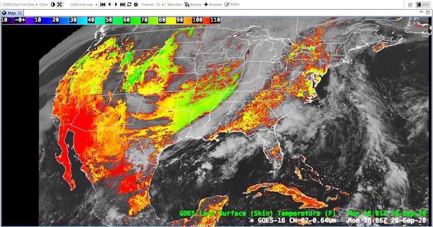
View GOES-R Imagery with AWIPS
● AWIPS (Advanced Weather Interactive Processing System) is the software used by the National
 Weather Service (NWS) to display and analyze meteorological data.
● Unidata developed and supports a modified non-operational version of AWIPS which is a free and
 open-source software that any user can download to view GOES-R Series data through a similar
 lens as weather forecasting offices (WFOs).
 ○ CAVE (Common AWIPS Visualization Environment) is a
 Java application which runs on Linux, Mac, and Windows.
 Follow these steps to download CAVE to your device.
 ○ AWIPS data can be accessed through the cloud using the
 EDEX Server. When prompted by the Connectivity
 Preferences Dialog, select the EDEX-cloud server.
 ○ Read Unidata’s CAVE User Manual to learn how to
 interact with and customize the AWIPS tools. See the
 GOES 16/17 Section for instructions specific to GOES-R
 channels, products, and RGB Composites.
 ■ For more detail, review the entire user manual,
 with particular attention to Section 2.2.
 ■ See p.56-63 for image display and time cadence Figure 5. The AWIPS display can overlay L2+ products and visible
 options, and p.53-55 for viewing preferences. imagery, such as Land Surface Temperature and Channel 2. 13

Access Data Files: NOAA CLASS
● The NOAA Comprehensive Large Array-data Stewardship System (CLASS) repository is the official site
 for accessing all available GOES-R Series Products.
 ○ Begin by selecting the product of interest from the search bar, such as GOES-R Series ABI Products (GRABIPRD)
 (partially restricted L1b and L2+ Data Products).
 ○ Use the Temporal and Advanced Search options to filter the data by time, date, satellite, geographic scale, and
 product. It is possible to include up to 10,000 files in an order. Click “Quick Search and Order”, then “Register”.
 ○ Fill in your contact information to create a Guest User Profile. Once you are logged into CLASS as a guest, the option
 to “Place Order” will appear. If you are a returning CLASS user, log in before beginning your data search.
 ○ When the order has been processed (up to 48 hours for large order sizes), instructions will be sent to the email
 address provided. The email will offer two options for accessing the file(s):
 ■ 1. Authenticate and download from CLASS via FTPS. This requires a robust FTP client. Use “anonymous” as
 the FTP user ID, and your email address as the password.
 ■ 2. Download each file individually from the CLASS website.
● A similar but easier website to navigate is NCEI's Archive Information Request System (AIRS).
 ○ Using the AIRS system, there is no need to set up an account.
 ○ It is possible to filter, search, and order up to 30 days worth of files, and access up to 1,000 files per order.
 ○ An email will be sent with download instructions for the processed files, with options for web and FTP downloads.
 ○ Another interface for downloading NCEI’s archive of GOES-R Series data is NCEI Dataset Search.
 14

Access Data Files: Amazon, Microsoft, OCC
● Amazon Web Service (AWS) - ABI L1b and L2+, GLM L2+, and SUVI L1b products are available in
 AWS S3 Buckets. These open datasets can be accessed by the public from AWS for free.
 ○ User interfaces for browsing and downloading the available products:
 ■ The AWS S3 Explorer interface can be used to browse the GOES-16 and GOES-17 buckets.
 ■ Alternatively, users with AWS accounts can browse the buckets via the AWS S3 Console.
 ■ The "GOES-16/17 on Amazon Download Page," created by Brian Blaylock, Ph.D., offers product filtering
 by satellite, domain, product, date and time through its comprehensive user interface.
 ○ Options for scripted/bulk downloading:
 ■ AWS Command Line Interface, rclone (see rclone tutorial for GOES data access) and the Python s3fs
 library (see Slide 17 for more information on using Python to download data).
 ○ See the README file under “Documentation” on the AWS page for GOES-specific instructions and file naming.
● Microsoft Azure - Two GOES-16 ABI Full Disk products are stored in a Azure blob container.
 ○ The products currently available are L1b Radiances and L2+ MCMI, which can be accessed from Azure for free.
 ○ Under the “Data access” tab, a demo notebook shows how to retrieve a file from blob storage and visualize the
 image with Python.
● Open Commons Consortium (OCC) - Stores a 100 TB rolling archive of GOES-16 data (~ 8 months),
 the products stored are ABI L1b and ABI L2+ CMI and MCMI.
 ○ OCC recommends using the AWS CLI or the python boto library, to access the data.
 15

Access Data Files: Google Cloud
● Google Cloud - ABI L1b and L2+, GLM L2+, and SUVI L1b products are available in two different
 buckets for GOES-16 and GOES-17.
 ○ GOES-R data can be browsed and pulled directly from the Google Cloud website. The data itself is stored in a
 Google Cloud Storage Bucket, while the indexed metadata is available in BigQuery.
 ○ The buckets can be filtered by product name and date, but be prepared with the product abbreviation and the
 day-of-the-year of interest, because there are few descriptors on the Google Cloud website.
 ○ Downloading the data requires authentication with a Google account (not Google Cloud specific).
 ■ Without a Google account, data access is still possible using a Cloud Storage API link.
 ○ BigQuery offers 1TB of querying per month for free. Additionally, a Google Cloud free trial provides $300 in
 credit, valid for 90 days, which can be used to explore other Google Cloud services.
 ■ Follow the “How to process weather satellite data in real-time in BigQuery” tutorial to visualize GOES-R
 data using Google Cloud and the gsutil command-line utility.
● Google Earth Engine (GEE) - A cloud-based platform for geospatial analysis. This service runs through
 Google Cloud, and pulls GOES-R datasets from the Google Cloud buckets.
 ○ Only two GOES-R L2+ products are currently available in the GEE Data Catalog. The products are Multi-band
 Cloud and Moisture Imagery (MCMI) and Fire Detection and Characterization (FDC).
 ○ Apply for a free GEE account to use this platform. It may take one-to-two days for the account to get approved.
 ○ See Slide 22 for more information on how to use GEE as a tool for image analysis and visualization.
 16

Use Python to Retrieve Data from AWS
● The following sample scripts demonstrate two different ways to retrieve GOES-R files from AWS using
 Python. The scripts must be edited to use the correct prefix for the file of interest.
 ○ For GOES-R file naming conventions, see the AWS README documentation.
● Script #1: “Visualize GOES-16 Data from S3” by Hamed Alemohammad
 ○ This script bypasses downloading data to a local device by pulling data directly from the AWS S3 Bucket, visualizing
 the data, and saving the image as a png. Recommended edits to Script #1 follow, based on a 1/6/21 review.
 ○ In [2]: Adjust information to reflect the specific product/date/file of interest. Be wary that not all products have
 data for multiple bands (if not, remove “band” attribute), or have images for every date.
 ○ In [5]: Change “M3” to “M6” (mode 3 to mode 6) if the imagery of interest was created after April 2, 2019.
 ■ This reflects the switch in ABI’s default scan mode. See Slide 7 for more information on scan modes.
 ○ In [8]: Change “Rad” to other variable name, if the product of interest is not an ABI L1b Radiance Product.
● Script #2: “Download GOES AWS” by Brian Blaylock
 ○ This simple script demonstrates how to do a scripted download of GOES-R files from AWS using anonymous
 credentials. Files are stored at a local directory. Recommended edits to Script #2 follow, based on a 1/6/21 review.
 ○ Line 12 : Adjust the bucket name from ‘'s3://noaa-goes16/' to GOES-17 if applicable.
 ○ Line 17 : Correct the prefix from ‘'noaa-goes17/ABI-L2-MCMIPC/2019/240/00/' to the file of interest.
● The GOES-2-Go and goespy Python packages can further streamline the download (see Slide 21).

 17

Part 3.

 How Can I Display the Data?

 18

Visualize with Command Line: Geo2Grid
● The free CSSP Geo2Grid software package is a set of command line tools which
 facilitate the creation of projected satellite images, developed at CIMSS/SSEC.
● Installation and setup:
 ○ Install the Geo2Grid software package on a device running Anaconda/Miniconda.
 ○ In command line, run: conda create -c conda-forge -n geo2grid
 polar2grid , then conda activate geo2grid.
 ○ Download ABI L1b files of interest, and store in a local directory.
● Use the ABI L1b Reader to read data, and write to single band GeoTIFF files:
 ○ geo2grid -r abi_l1b -w geotiff -f 
● RGB composites can be be generated by specifying -p [product] (Figure 6):
 ○ geo2grid -r abi_l1b -w geotiff -p true_color -f
 
 ○ Products: True color*, natural color* air mass, ash, dust, fog, and night microphysics.
 ○ *These RGBs are ratio-sharpened, enhanced, and an atmospheric correction is applied. Figure 6. GeoTIFFs created using
● Other functions include: remapping data to a different projection, subsetting data Geo2Grid. 6a (top): GOES-16
 CONUS true color. 6b (bottom):
 to a geographic bounding box, and setting the file output format to a png. GOES-17 PACUS natural color.
● For more information, see Geo2Grid Basics and Examples for Working with ABI
 Data. 19

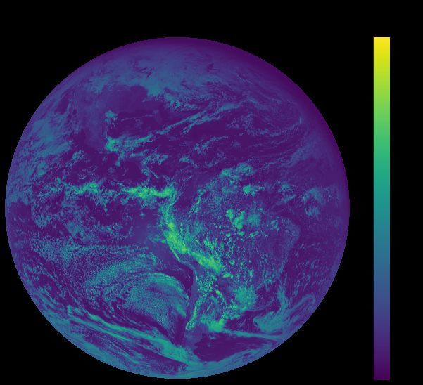
Visualize with Python: Basics
● Import data to Python directly from AWS (see Slide 17 and Slide 19 for
 examples), or from a local directory.
● Visualize GOES-R imagery using Python packages: xarray and matplotlib.
 ○ Xarray processes GOES-R data as multidimensional arrays. Matplotlib plots data
 to generate images with legends. Figure 7a adapted from Script #1 output.
● Georeference GOES-R imagery using Cartopy package.
 ● Cartopy helps georeference data, so that geographic features
 like state borders can be overlaid. Cartopy should be used
 instead of Basemap, a package that is now deprecated.
 ● Script #3: “Mapping GOES-16 True Color” by Brian Blaylock.
 An excellent tutorial with step by step explanations for how to
 render and georeference a GOES -16 true color image. Figure
 7b created by following this script.
 ● Script #4: “Accessing GOES-16 data on Azure.” A nearly
 identical script, but with code instructing how to access
 GOES-16 data from blob storage on Azure.
Figure 7. GOES-16 visualized with Python. 7a (top) ABI L1b Channel 2 Full Disk
Radiances from Jan 5th, 2021. 7b (bottom): True Color CONUS from June 4th, 2020.
 20

Visualize with Python: Custom Packages
● The prior Python examples employ widely-used packages for processing any environmental data.
 However, by using more specialized Python packages, it is possible to process and visualize GOES-R
 imagery with fewer lines of code. Follow the respective installation guides and documentation.
● Satpy - a Python package for reading, writing and manipulating satellite imagery by the PyTroll Team.
 ○ Satpy processes GOES-R data using specialized readers: abi_l1b, abi_l2_nc, and glm_l2. Satpy’s capabilities include
 generating composites, extracting measured values, resampling to a uniform grid, slicing and subsetting scenes.
 ○ See Satpy’s “Quickstart” webpage for an overview, and “Reading Data with the Scene” for an ABI L1b example.
 ○ Script #5: “GOES-16 Mosaic”- Pull files from AWS, or load local files, then join all 16 bands with ImageMagick.
 ○ Script #6: “GOES-16 ABI - True Color Animation” - Combine single ABI timesteps to create an mp4 video file.
● GOES-2-go - a Python package created by Brian Blaylock, Ph.D.
 ○ Downloads and reads ABI and GLM data from AWS. A user may retrieve the latest GOES-R data, select images
 from a specific time and date, or choose a series of images from a date range.
 ○ Creates multispectral RGB composites, based on recipes from RAMMB/CIRA, such as True Color, Natural Color,
 Air Mass, and Day Cloud Phase Distinction. For some examples, see Script #7: “RGB Demo Notebook”.
● goespy - a Python package created by Steven Pestana and Paulo Alexandre Mello.
 ○ Simplifies downloading from AWS with two functions: the ABI_Downloader and the GLM_Downloader.
 ○ Script #8: “Downloading and plotting GOES-R imagery with goespy and xarray” - Demonstrates goespy utility.
 21

Visualize with Earth Engine
● Google Earth Engine (GEE) is a cloud-based platform for
 geospatial data analysis. The following list summarizes the
 advantages of imagery processing using GEE:
 ○ The GOES-R imagery stored in the GEE Data Catalog is already
 georeferenced. Therefore, it only requires a few lines of script to
 display an image accurately (Figure 8).
 ○ GEE provides advanced image processing tools designed for
 satellite imagery analysis, offered through several APIs.
 ○ The GEE Data Catalog stores many datasets, including imagery
 from MODIS, Landsat, and Sentinel, which are updated daily.
 Synthesizing dissimilar satellite products is possible in GEE.
 ○ GEE takes advantage of Google’s infrastructure to execute high
 speed parallel processing. This is helpful for handling large Figure 8. GOES-16 CONUS False Color image on June 12th,
 collections of images, without using local computing resources. 2020, visualized using GEE.
 ○ For an introduction to GEE, check out the GEE Community Tutorials.
● Be aware of the following:
 ○ To use this platform, it is necessary to apply for a free GEE account, which may take a day or two to get approved.
 ○ Two GOES-R Series L2+ products are currently available in the GEE Data Catalog: Multi-band Cloud and Moisture
 Imagery (MCMI) and Fire Detection and Characterization (FDC). Sample scripts available for products at links.
 22

Technique: Radiance to Reflectance
● When using the L1b Radiance product, it may be beneficial to convert from the unit radiance, which
 takes into account the solar irradiance and Earth-Sun distance. For the reflective bands (1-6), convert
 to reflectance. For the emissive bands (7-16), convert to brightness temperature (Kelvin).
● Reflectance conversion equation: reflectance ρ v = kappa factor κ * radiance Lv
 ○ The kappa factor is included in the metadata for every L1b file, stored as the variable 'kappa0'
 ○ For more information on the reflectance conversion, or how to convert to brightness temperature, see the PUG:
 Volume 3: L1b Products, Revision 2.2, pages 27-28.
● Script #9: “True-Color Image: GOES-R ABI L1b Radiances” by Danielle Losos.
 ○ This Jupyter Notebook demonstrates several useful techniques for processing and visualizing the L1b Radiance
 product to create a georeferenced RGB True-Color image.
 ○ Compare to the Script #3 methodology for creating true color images from the L2+ MCMI product.
 ■ See Slide 24 for background on using multiple bands to generate true-color composite images.
 ○ Alternative approach for converting radiance to reflectance values is documented in the tutorial: “Jupyter
 Notebook for Working with GOES-16 Data” by OCC . However, this script errs in using constant values to
 convert between radiance and reflectance. It is recommended to always use the coefficients embedded in that
 particular image’s metadata for conversion to reflectance or brightness temperature.
 ■ A section of the OCC script shows how to visualize Geostationary Lightning Mapper (GLM) point data.

 23

Technique: Generating Composites
● "Band stacking" is the process of overlaying certain bands to create composite imagery. Read “Satellite
 imagery RGB: Adding Value, Saving Time” for background on how composites aid weather forecasting.
● A popular composite image type is an RGB True Color, which uses red, green, and blue wavelength
 imagery to mimic the appearance of the Earth to the human eye.
 ○ GOES-R has blue and red visible channels (bands 1 and 2), but not a green visible channel. The near infrared (NIR)
 channel (band 3) can serve as a proxy for the green band. Script #3 shows how to create an RGB True Color image
 from bands 1, 2 and 3 of the MCMI product. MCMI is a single file with all 16 bands resampled to 2 km resolution.
 ○ Using three separate CMI files for the three bands is less data intensive and achieves a higher resolution. However,
 band 2 has 0.5 km resolution while bands 1 and 3 have 1 km resolution, which makes multi-band operations difficult.
 Thus, it is necessary to resample band 2. Script #9 demonstrates how to resample using a Rebin function.
● Other GOES-R RGB composites do not simulate true color, but instead highlight various atmospheric
 and surface features, such as the Air Mass RGB , Day Cloud Phase Distinction RGB, and Dust RGB.
 ○ Satpy and GOES-2-Go packages automate the generation of common GOES-R composites.
● Another common composite is NDVI (normalized difference vegetation index). This index determines
 vegetative health by finding a the difference between a pixel’s reflectance in red and NIR wavelengths.
 ■ Script #10: Shows how to easily calculate NDVI of a Landsat image in Python using the module Earthpy. To
 calculate NDVI using a GOES-R image, substitute band 2 as the red band and band 3 as the NIR band.
 24

Part 4.

 How Can I Process the Data
 Using GIS?

 25

Make GOES-R Series Data GIS-compatible
 ● The native format for GOES-R products is netCDF files (see Slide 31) which are not always compatible
 with GIS. To process products using GIS software, it may be necessary to change the data format.
 ● Raster and vector models are the two primary ways to represent geospatial data for visualization in GIS.
 ○ Raster Models: grids of rectangular pixels, with each pixel assigned a value that corresponds to
 the measured environmental feature. To learn more, read “What is raster data?”.
 ■ Since GOES-R netCDF files store variables in multidimensional arrays, most products
 can be converted easily to raster file formats (Slide 27).
 ■ Over a hundred raster file types are supported by the open-source platform QGIS.
 Common formats for storing satellite imagery include TIFF, IMG, GRID, JPEG, JP2,
 BMP, GIF, PNG, BIL/BIP/BSQ, and DAT.
 ○ Vector Models: points, lines, or polygons used to explicitly delineate the boundaries of
 environmental features. Each geometry (a point/line/polygon) may have associated attributes
 which describe the characteristics of the feature. For more information, read “Vector Data”.
 ■ GOES-R NetCDF multidimensional arrays cannot be modeled by vectors without
Source: transforming the data.
Saylor Academy
 ■ Shapefiles are the most widely used vector format and are compatible with any GIS
Figure 9. This graphic shows how platform. Other file formats for storing vector data include GeoJSON, KML/KMZ, TIN,
point/line/polygon vectors and raster and DXF.
grids model surfaces differently.
 26

Convert NetCDF files to GeoTIFFs
● NetCDF files are compatible with select GIS platforms. QGIS Version 3.2+ can handle some GOES-R
 products. Using QGIS 3.14: go to Add Layer > Add Raster Layer, then select a variable when prompted.
● GeoTIFFS are regarded as the industry standard for georeferenced raster data.
 The conversion of GOES-R netCDF arrays to single-band GeoTIFF rasters can be
 accomplished in command line, using GDAL or Geo2Grid (see Slide 19).
 ○ Install the package Geospatial Data Abstraction Library (GDAL). Use the command
 gdal_translate NETCDF:"Input_file.nc":Variable_name Output_file.tif
 ○ For example: gdal_translate NETCDF:"OR_ABI-L1b-RadC-M6C01_G16_s2021
 0010016176_e20210010018549_c20210010019000.nc ":Rad Sample_Output.tif
● The collection of scripts, “GOES-R NetCDF to GeoTIFFs” by Danielle Losos, can
 assist with batch retrieval and conversion. These scripts automate the file
 download by pulling data from a given satellite, product, and date from AWS. Figure 10. GOES-16 L2+
 ○ Script #11: “L1b Channel Loop” – Loops through the 16 netCDF files contained in an ABI CMI clipped to the
 L1b Radiance product, and converts each to a GeoTIFF. Minnesota border,
 ○ Script #12: “L2 Products” – Visualizes and converts the chosen GOES-R L2+ ABI product converted to a GeoTIFF,
 variable, such as Cloud Top Height, from a netCDF file to a GeoTIFF. and visualized in QGIS
 ○ Script #13: “Clip with Shapefile” – Clips a netCDF file image down to a shapefile boundary, using Script #13.
 ie. a state border, and saves the region of interest as a GeoTiff (Figure 10).
 27

Transform Discrete Data to Shapefiles
● Discrete data, also known as thematic or categorical data, is used to represent features that have
 defined boundaries. Vector models are better suited for discrete than continuous variables. Read
 “Discrete and Continuous Data” to learn more about the difference between these data types.
 ○ Several GOES-R L2+ products have discrete variables, including the Clear Sky Mask which provides a binary
 classification for each pixel: “clear” or “cloudy”; Aerosol Detection; and Cloud Top Phase.
 ○ Most GOES-R products have a Data Quality Flag (DQF) layer, a discrete variable which classifies each pixel’s usability
 into categories like “good quality”, “conditionally usable” or “out of range”.
● Script #14: “Discrete variable to shapefile” by Danielle Losos.
 ○ This script transforms GOES-R products to shapefiles by polygonizing gridded data. A vector polygon is created for
 each connected region of
 pixels in the array sharing a
 common value.
 ○ For example, the Clear Sky
 Mask can be polygonized
 to a vector layer where
 each polygon has an
 attribute equal to 0 for
 cloud-free or 1 for Figure 11. Clear Sky Mask vector layer
 cloud-covered (Figure 11). (left image) is used to mask an RGB-false
 color raster in QGIS (right image). 28

Transform Continuous Data to Shapefiles
 ● Continuous data represents variables that change progressively across surfaces. Most GOES-R
 products contain continuous variables, like radiance, reflectance, temperature or pressure.
 ○ Continuous variables are not modeled well by vector data. Transforming satellite imagery to vectors requires
 generalization of data into categories (ie. discrete intervals) which results in a loss of detail and accuracy.
 ○ However, certain geospatial analytic operations can only be performed on vector data.
 ● Script #15: “Continuous variable to contour to shapefile” by Danielle Losos.
 ○ This script converts GOES-R products to shapefiles by first transforming the continuous variable into a contour
 plot of n discrete intervals. Next, the concentric rings of the contour plot are converted into shapefile polygons.
 ○ As the number of contour intervals, n, increases, the accuracy of the vector model improves (Figure 12). The trade
 off for a higher n is a longer processing time and ultimately a larger file size.

Figure 12. GOES-16
CONUS L2+ Land
 n=5 n = 15 n = 50
Surface Temperature
visualized as a contour
plot with 5, 15, and 50
discrete intervals.

 29

Part 5.

 Frequently Asked Questions

 30

How are GOES-R Series files formatted?
● GOES-R Series product files use the netCDF-4 format, a general-purpose scientific data file format.
● More details on netCDF files:
 ○ GOES-R Series products may have any of the following types of attributes
 ■ title : a global attribute that is a character array providing a succinct description of what is in the dataset.
 ■ Conventions : a global attribute that is a character array for the name of the conventions followed by the product.
 ■ long_name : long descriptive name for each variable.
 ■ _FillValue : a scalar value that identifies missing data.
 ■ Valid_range : a delimited vector of two numbers specifying the minimum and maximum valid values for the variable to
 which it is attached.
 ■ scale_factor and add_offset : these attributes are used together to provide simple data compression to store
 floating-point data as small integers in a product data file.
 ■ units : a character string that specifies the units used for the variable’s data.
 ○ A netCDF file also includes the dimensions that are used to size dimensional variables.
 ○ The netCDF ABI L1b/L2+ gridded product files are compressed to reduce the file size. For information on how to
 unpack data, see Slide 32. For more details on netCDF files, refer to the PUG Volume 1, Revision 2.2, pages 8-14.
● Other file formats:
 ○ Flexible Image Transport System (FITS) format is used alongside netCDF for the SUVI Solar EUV Imagery product.
 ○ Unix text file format is used in a small subset of the Level 1b and 2+ semi-static source data files.
 ○ Hierarchical Data Format (HDF) is used for several Level 1b semi-static source data files.
 31

How do I pre-process GOES-R Series data?
● GOES-R Series data are packed in compressed files, which must be “unpacked” for integer analysis. Images
 can be visualized without unpacking, since scaled integers are still proportional to each other.
● What is packed data?
 ○ In order to minimize file size, many of the ABI L1b/L2+ products use 16-bit scaled integers for physical data quantities
 rather than 32-bit floating point values.
 ○ To convert data back to the actual value associated with the physical quantity, the user must multiply by a scale factor
 and add an offset to the 16-bit scaled integer.
● How do I unpack data?
 ○ To unpack the data, apply the attributes using the following equation:
 unpacked_value = packed_value * scale_factor + add_offset
 ○ The variables ‘scale_factor’ and ‘add_offset’ are included in the metadata for each file. The scale factor is calculated
 with the formula (Max Value - Min Value)/65530, and the offset is the product’s expected minimum value.
 ○ Here is a sample conversion for band 8: Brightness temperature(Kelvin) = (2,305.05 * 0.04225) + 138.05 = 235.44 K
 ○ Before unpacking, check to ensure that the program in use is not automatically applying the scale factor and offset.
● How do I remove data that is fill, out of range, or missing, from the image?
 ○ These faulty data types can be masked using data quality flags (DQFs), convention attributes which associate integer
 values with a categorization of the data quality.
 ○ For more information on packed data or DQFs, see the PUG Volume 1, Revision 2.2, pages 21 or 16, respectively.
 32

How are ABI L1b products georeferenced?
● The ABI uses a fixed grid whose native coordinate values are the
 East/West scanning angle and North/South elevation angle in units of
 radians relative to the location of the satellite.
 ○ The ABI fixed grid is a projection based on the viewing perspective of the
 idealized location of a satellite in geosynchronous orbit. This allows the
 same data points in every product to be at the same location on Earth.
 ○ The fixed grid is rectified to an ellipsoid defined by the Geodetic Reference
 System 1980 (GRS80) earth model.
 ○ For all ABI gridded L1b/L2+ products, the names of the coordinate variables
 are x (E/W scanning angle) and y (N/S elevation angle) (Figure 9).
 ○ Additionally, there is a “grid_mapping” attribute which is attached to data
 variables whose values are associated with specific earth locations.
 ○ For ABI L1b/L2+ gridded products, the grid mapping attribute specifies the
 projection (GRS80), the lat/lon origin of the projection, and a parameter that
 identifies the ABI scanning pattern.
 Figure 9. Every data point is plotted on the ABI
● Grid mappings coupled with the coordinate variables provide the fixed grid as a distance from the (0,0) origin, in
 means to determine the latitude and longitude of a data point. units x (East to West Scanning Angle) and y
 (North to South Elevation Angle).
 ○ See the PUG Volume 3: L1b Products, Revision 2.2, pages 8-26, for an
 explanation in greater depth. 33

Why are data not available on a given date?
● Cloud-based platforms have select L2+ Product availability.
 ○ Once a GOES-R Series product has reached provisional status, cloud-based platforms may release the product.
 ○ When there is demonstrated user interest in a product, vendors may backfill their archive to include the dates
 requested. This may include beta maturity levels of the product.
 ○ If there is no demonstrated user interest in the product, vendors may choose not to release the entire available
 collection. For this reason, collection length may vary between products on cloud-based platforms.
● To retrieve pre-provisional GOES-R Series products, search on NOAA CLASS to access the entire archive
 of products made available to users. CLASS stores products with beta, provisional, and full status.
● Occasionally, there is missing GOES-R Series data on select dates and times.
 ○ To investigate whether data is missing due to issues with data reception, check out the SSEC’s Monitoring Web Page.
 Follow these instructions for tips on how to navigate this website:
 1. First, select either GOES-16 or 17, then choose a date of interest at the top of the page.
 2. Each row represents the data quality of full disk, CONUS, and mesoscale images for every hour of the day.
 3. The “DB SSEC” section reports missing data due to GOES Rebroadcast (GRB) reception issues.
 KEY- light green: 100% received, yellow: 96 -100% received, light red: < 96% received, dark red: missing
 4. The “PDA via STAR” section reports missing data due to errors with Product Distribution and Access (PDA).
 KEY (same as above with two more categories)- blue & orange: data available from PDA but missing or late
 ○ Also, check out General Satellite Messages to see if there were any outages reported on that day (Search the date, i.e.
 “July 10, 2020”). 34

Other Questions and Contact
Other Questions

 ● For unanswered questions, try browsing the GOES-R Series FAQ Page or NCEI’s FAQ Page.
 ● For technical details on the satellites or products, the GOES-R Series Documents page has links to
 many helpful GOES-R documents, including the Product Definition and User’s Guides (Volumes 1-5)
 and the Product Algorithm Theoretical Basis Documents (ATBDs).

Contact

 ● Get in touch by emailing the Satellite Products and Services Division (SPSD) User Services at
 SPSD.UserServices@noaa.gov.
 ○ Please share your questions, concerns, or suggestions for how this GOES-R beginner’s guide
 could be more helpful.
 ● Show us how you are using GOES-R data in your own work by using #goesrguide when you post on
 social media!
 35

Appendix A: Acronym List
ABI - Advanced Baseline Imager FITS - Flexible Image Transport System NetCDF - Network Common Data Format
AIRS - Archive Information Request System FTP - File Transfer Protocol NIR - Near-infrared
ATBD - Algorithm Theoretical Basis Documents GDAL - Geospatial Data Abstraction Library NOAA - National Oceanic and Atmospheric
AWIPS - Advanced Weather Interactive Processing GEE - Google Earth Engine Administration
 System GIS - Geographic Information System NWS - National Weather Service
AWS - Amazon Web Service GLM - Geostationary Lightning Mapper OCC - Opens Commons Consortium
CAVE - Common AWIPS Visualization Environment GOES - Geostationary Operational PACUS - Pacific U.S.
CIMSS - Cooperative Institute for Meteorological Environmental Satellite PDA - Product Distribution and Access
 Satellite Studies GRB - GOES Rebroadcast PUG - Product User Guide
CIRA - Cooperative Institute for Research in the GRS80 - Geodetic Reference System 1980 RAMMB - Regional and Mesoscale Meteorology
 Atmosphere HDF - Hierarchical Data Format Branch
CLASS - Comprehensive Large Array-data L0/L1b/L2+ - Level 0/ Level 1b/ Level 2+ RGB - Red-Green-Blue
 Stewardship System MAG - Magnetometer SEISS - Space Environment In-Situ Suite
CMI - Cloud and Moisture Imagery SGPS - Solar and Galactic Proton Sensor
 MCMI - Multi-band Cloud and Moisture Imagery
CONUS - Continental U.S. SPoRT - Short-term Prediction Research and
 MESO 1/2 - Mesoscale Domain Sector 1/2
CSSP - Community Satellite Processing Package Transition Center
 MPS-HI/LO - Magnetospheric Particle Sensor -
DQF - Data Quality Flag SPSD - Satellite Products and Services Division
 High/Low
EHIS - Energetic Heavy Ion Sensor SSEC - Space Science and Engineering Center
 NASA - National Aeronautics and Space
EUVS - Extreme Ultraviolet Sensor SUVI - Solar Ultraviolet Imager
 Administration
EXIS - Extreme Ultraviolet and X-ray Irradiance WFO - Weather Forecast Office
 NCEI - National Centers for Environmental
 Sensors
 Information
FDC - Fire Detection and Characterization
 NDVI - Normalized Difference Vegetation Index Additional acronyms defined on the GOES-R Series
 Acronym Page. 36