Estimating Learning-by-Doing in the Personal Computer Processor Industry
←
→
Page content transcription
If your browser does not render page correctly, please read the page content below
Estimating Learning-by-Doing in the Personal
∗
Computer Processor Industry
†
Hugo Salgado
First Draft, May 2008
Abstract
I estimate a dynamic cost function involving Learning-by-doing in the
Personal Computer Processor industry. Learning-by-doing is an important
characteristic of semiconductor manufacturing, but no previous empirical
study of learning in the processor market exists. Using a new econometric
method, I estimate parameters of a cost function under a Markov perfect
equilibrium. I
nd learning rates between 2.54% and 24.86%, and higher
production costs for AMD compared to INTEL, the two
rms in the market.
Around 12% of the dierences in costs between
rms is explained by the
lower learning that AMD obtains given its lower production levels. These
learning rates are lower than those of other semiconductors products and
they indicate that when the
rms begin the production in the fabs they
have already advanced in their learning curve and most of the learning occurs
before-doing in the development facilities.
∗
This paper is a draft of the third chapter of my dissertation. In the
rst chapter I
estimate a random coe
cient model of demand and analyze the importance of the Intel
brand in demand for CPU. In the second chapter I analyze dierent measures of market
power in a dynamic model of
rm behavior. Please do not cite or circulate. All comments
are welcome.
†
PhD. Candidate, Department of Agricultural and Resource Economics, University of
California at Berkeley. e-mail: salgado@berkeley.edu
11 Introduction.
The Central Processing Unit (CPU) is the brain of the personal computer
(PC), performs all of the information processing tasks required for comput-
ing. The technological development of the CPU, the most important PC
component, has been one of the keys to growth in the PC industry over the
last three decades. Two of the clearest trends in the CPU and the PC mar-
kets are the sustained increase in product quality and a steep decrease in
price over time. Several reasons have been cited for these trends, the most
important of which are strategic interactions between
rms, a continuous in-
troduction of new, improved products, and the existence of learning-by-doing
in the production process.
The evidence for learning-by-doing in the semiconductor industry is abun-
dant. It has been well documented that learning plays an important role in
the semiconductor industry due to signi
cant reductions in failure rates.
When a new product is introduced, the proportion of units that passes qual-
ity and performance tests (yield ) could be as low as 10% of the output.
Production experience and adjustment in the process over time decrease
failure rates, increasing yields up to 90%, which reduces unitary production
costs over the lifetime of a product (Irwin and Klenow, 1994). The empirical
applications of learning in the semiconductor industry have concentrated on
memory manufacturing (Baldwin and Krugman 1988; Dick 1991; Irwin and
Klenow 1994; Gruber, 1996, 1999; Hatch and Mowery, 1999; Cabral and
Leiblein, 2001; Macher and Mowery, 2003; Siebert, 2008), and even though
memory and CPU production processes are subject to the same type of
2learning economies, no evidence exists of the importance of learning in CPU
manufacturing. Surprisingly, while most of the studies in the PC CPU in-
dustry recognize the existence of learning in the manufacturing process, they
have focused on other characteristics of the market and ignored cost deter-
minants and learning-by-doing as a key component of the industry (Aizcorbe
2005, 2006; Gordon 2008; Song 2006, 2007).
In this paper I estimate the extent of learning-by-doing in the PC CPU
industry using a new econometric method by Bajari, Benkard and Levin
(2007). Compared to previous emprirical studies of learning-by-doing, this
method requires weaker assumptions regarding
rms dynamic behavior. The
method employs a closed loop approach, which allows me to control for how
the
rms think their rivals will react in the future to changes in their current
behavior. Additionally, the method has several computational advantages
because it makes use of simulations that (1) do not require neither to
nd
an algebraic solution for the equilibrium of the game, and (2) do not require
me to choose amongst possible multiple equilibria. Instead, the method as-
sumes that the observed behavior is the equilibrium that
rms decide to play.
This method makes it feasible to estimate learning rates while controlling for
strategic interactions among
rms, heterogeneous preferences of consumers,
and periodic introduction of new, dierentiated products, into the market.
I use a proprietary dataset from In-Stat/MDR, a research company special-
izing in the CPU Industry that is the data source for all the analysis and
forecasting done in the PC CPU market. It contains detailed quarterly ship-
ment estimates and prices for 29 products by AMD and INTEL over 48 time
periods from 1993 to 2004.
3The analysis in this paper diers from the previous literature in several
ways. Most previous studies have assumed that products are homogeneous
and that
rms are symmetric; in most cases, they have also taken demand
elasticity as a parametric assumption (one exception is Siebert, 2008). In
this paper I use estimates from a random coe
cient demand model (Salgado,
2008) which allows me to control for the existence of dierentiated products
and for heterogeneity of preferences among consumers. This also makes it
possible to analyze strategic interactions among
rms in a complicated game
in which
rms choose prices for each of their available dierentiated products
under dynamics given by learning-by-doing.
The results show that there are large dierences between
rms' estimated
production costs, with AMD's average costs more than twice Intel's average
costs. These dierences are explained by both a higher production cost upon
introduction of a product and a lower learning gain due to lower production.
The average estimated learning rates
uctuate between 2.54% and 17.01%
for AMD and between 4.74% and 24.86% for Intel, which are lower than
those found in other empirical studies of semiconductor products, which
have found average learning rates of 20%. This dierence in learning rates
suggests that in the CPU market,
rms transfer the production process from
the development facilities to the production fabs succesfully once they have
already advanced in their learning curve.
The structure of the paper is as follows. Section 2 reviews the most
relevant studies, both theoretical and empirical, in the learning-by-doing
literature. Section 3 describes a structural model that captures the charac-
teristics of the market I am interested in analyzing. Section 4 presents the
4econometric method and explain how can it be applied to estimate the rates
of learning in CPU manufacturing. Section 5 presents the results and the
ndings and section 6 concludes.
2 Literature Review
The learning-by-doing hypothesis states that in some manufacturing pro-
cesses, cost are reduced as
rms gain production experience. This hypothesis
originated with Wright (1936), who observed that direct labor costs of air-
frame manufacturing fell by 20% with every doubling of cumulative output.
Since then, many empirical studies have analyzed the existence of learning-
by-doing in a variety of industrial settings, and a number of theoretical pa-
pers have analyzed dierent implications of learning for endogenous growth,
market concentration, and
rms' strategic interactions (Lee 1975, Spence
1981, Gilbert and Harris 1981, Fudenberg and Tirole 1983, Ghemawat and
Spence 1985, Ross 1986, Dasgupta and Stiglitz 1988, Mookherjee and Ray
1991,Habermeier 1992, Cabral and Riordan 1994, Cabral and Leiblein 2001).
Theoretical analyses have shown that learning-by-doing could create en-
try barriers and strategic advantages for existing
rms (Lee 1975, Spence
1981, Ghemawat and Spence 1985, Ross 1986, Gilbert and Harris 1981) and
facilitate oligopoly collusion (Mookherjee and Ray, 1991). Gruber (1992)
presents a model in which learning-by-doing could generate stability in mar-
ket share patterns over a sequence of product innovations, given the existence
of leaders and followers in the market. Cabral and Riordan (1994) show that
learning-by-doing creates equilibria with increasing dominance of one
rm
5in the market and might generate predatory pricing behavior by the leaders
who use their cost advantage to prevent new
rms from entering the market.
Besanko, et.al. (2007) analyze a model of learning-by-doing to explain the
incentives that
rms have to price strategically, showing that
rms might
price more aggressively in order to learn more quickly and gain dominance
over competitors, as well as to prevent their competitors from learning.
The existence of learning-by-doing in the semiconductor manufacturing
process has been widely analyzed. The source of learning has been attributed
to the adjustments that are necessary to obtain high productivity during
fabrication. The semiconductor production process is based on hundreds
of steps in which circuit patterns from photomasks are imprinted in silicon
wafers and then washed and baked in several layers, thus forming the millions
of transistors that allow the chip to function as an information processing
device. These steps must be performed under precise environmental condi-
tions that are controlled and adjusted continuously. When a product is
rst
transfered from the development labs to full production in the fabs, the num-
ber of units that pass control quality tests (yield) is very small, and several
ne-tuning steps need to be taken in order to obtain high yields. Given that
the production cost of a wafer is independent of the number of working chips
at the end of the product line, low yields mean higher production cost per
working unit. It is the increase in the yield rates that generates reduction in
the production cost of the
nal products. Hatch and Mowery (1998) analyze
detailed production data on unitary yields for a number of semiconductor
chips and conclude that both cumulative production and engineering analy-
sis of the production output are the sources of improvements in yield rates
6over the lifetime of the products.
The most common speci
cation in the empirical analysis of learning-by-
doing is based on a constant learning-elasticity
log ct = α + η log Et−1 + εt (1)
Where ct represents unitary production costs, usually assumed constant
within a period, and Et−1 re
ects some measure of production experience,
usually proxied by cumulative production. Using this speci
cation, the goal
of the empirical analysis is to estimate the constant experience-elasticity η
and use it to measure a learning rate, which measures the percentage reduc-
tion in average cost when cumulative production doubles, de
ned by:
c(Et ) − c(2Et )
rt ≡ = 1 − 2η (2)
c(Et )
In a seminal empirical paper on learning-by-doing in the semiconductor
industry, Irwin and Klenow (1994) construct a structural model of learning-
by-doing and estimate learning spillovers among seven generations of DRAM .
1
They focus the analysis on estimating how the cumulative production of each
product, as well as the cumulative production of all other products, aects
unitary average costs. Using quarterly data from 1974 to 1992, they
nd
average learning rates of 20% for the dierent products. They also
nd that
rms learn three times more from internal cumulative production than from
spillovers from other
rms experience and that cumulative production of
1
Dynamic Random Access Memory, one of the volatile memory devices used in com-
puters.
7previous generations has weak eects on the costs of new products. In their
model, they assume that products are homogeneous and
rms are symmet-
ric, and they solve for the Cournot equilibrium of the dynamic game under
an open-loop assumption. This assumption means that
rms commit to a
path of production over the future in an initial time period and that they
do not modify this path in the future. This implies that
rms will not ad-
just their plans over time depending on how the game evolves, nor will they
react to changes in their competitors' behavior. If the game under analy-
sis has some random components, as in our application, this assumption is
clearly not valid. The authors estimate the parameters of the cost function
with a GMM method using instruments and the
rst order conditions of the
dynamic problem. They also propose the use of a non-linear least squares
(NLLS) method that assumes a functional form for the dynamic cost , which
2
facilitates the estimation process and avoid the need of valid instruments.
Gruber (1998) applies the NLLS method to the production of EPROM
3 chips
and
nds learning rates between 23% and 30%.
More recently, Siebert (2008) explore learning-by-doing recognizing that
dierent generations of products are competitors in the demand side of the
market. He estimates a dynamic oligopoly model under a Markov perfect
equilibrium, in which
rms choose quantities of each available product. He
assumes that
rms base their decisions only on industry total cumulative
production; furthemore, he assumes that products are homogeneous within
2
The dynamic cost is the sum of current period marginal cost and the shadow value of
learning
3
Erasable Programmable Read-only Memory, one of the memory chips that can keep
information even when the source of power is interrupted. They were used as BIOS chips
in old PC and other electronics.
8a generation, but that sales of other generations have dierentiated eects
on prices. He also implicitly assumes that the demand function is common
across generations of products and assumes a functional form for the dynamic
marginal cost. As in Irwin and Klenow (1994), he uses the
rst order condi-
tions of the dynamic game in a GMM approach to estimate the parameters
of the cost function. The author recognizes the externality that production
decisions generates over the demand of the other
rm' products and
nd that
ignoring this eect generates biased estimates of learning rates. He found
learning rates of 34% when taking into account multiproduct eects and 20%
when ignoring these eects.
As stated in the introduction, all of the empirical evidence of learning-
by-doing in the semiconductor industry comes from memory chips manufac-
turing. This has been mainly because the market in memory chips is more
competitive, and market data have been readily available since the 1970s.
Based on new data availability for the PC CPU market, a more recent litera-
ture has studied dierent characteristics of the CPU market. Aizcorbe (2005)
analyzes a vintage model of new product introduction; Aizcorbe (2006) ex-
amines price indices during the 1990s; and Song (2007), Gordon (2008) and
Salgado (2008) analyze dierent models of demand to measure consumer wel-
fare, demand for durable products and the eects of advertising and brand
loyalty on demand, respectively. All these papers have ignored the existence
of learning-by-doing as a key component of the manufacturing process.
93 The Model
This section presents a structural econometric model that captures the most
important characteristics of the PC CPU industry. There are two
rms in
the market, AMD (A) and INTEL (I), with ntA and ntI products available in
period t. Products are dierentiated in terms of their quality, which evolves
stochastically over time, where quality of product i in period t is given by
kit . Products enter and exit the market exogenously to the
rms' pricing
decision. It is common knowledge that product i enters the market at time
ti0 and exits the market at time tiT . Firms choose prices for each one of the
available products i ∈ Ijt (the set of products available for
rm j at time t).
In the remainder of this section, I present details of the three main com-
ponents of the model: demand, cost functions, and the equilibrium concept
of the dynamic game.
3.1 The model of demand
Demand is modeled using a random coe
cient model with quality being the
only relevant product characteristic. As in Salgado (2008), I use a CPU
performance benchmark that measures the speed at which each CPU can
complete a number of tasks. Even though a more detailed characterization
of the products is possible (using for example clock speed, amount of cache
memory, front speed bus and other characteristics) there is a strong corre-
lation between all of these characteristics and the index of performance. I
prefer to use a single characteristic to reduce the number of state variables
and facilitate the estimation of the dynamic game.
10Following Nevo (2000), I present the main components of a random co-
e
cient demand model for the CPU industry. We observe the CPU market
in t = 1...T time periods. The market has L potential consumers that must
decide either buy one of the available products or not. We observe aggre-
gate quantities, prices, and a measure of quality (kit ) for each product. The
indirect utility of consumer l from choosing product i at time t is given by
ulit = αl (yl − pit ) + βl kit + ξit + εlit
(3)
l = 1 . . . L, i = 1 . . . It , t = 1 . . . T
where yl is the income of consumer l, pit is the price of product i at time
t, kit is the measure of quality of product i in time t, ξit is a product charac-
teristic observed by consumers and
rms but unobserved by the researcher,
εlit is a random term with a type I extreme value distribution, αl is con-
sumer l's marginal utility from income and βl is consumer l's marginal utility
from product quality. Additionally, we assume that the taste coe
cients are
independent and normally distributed among the population. Under this
assumption, the preferences over income and quality of a randomly chosen
consumer can be expresed as:
αl α + σα vαl
=
βl β + σβ vβl
vαl , vβl ∼ N (0, 1)
The demand speci
cation also includes an outside good, which captures
the preferences of consumers who decide not to buy any of the available
11products. The indirect utility from this outside good, which is normalized
to zero, is:
ul0t = αl yl + ξ0t + εl0t = 0
The indirect utility function in (3) can be written as
ulit = αl yl + δit (pit , kit , ξit ; α, β) + µlit (pit , kit , vl ; σ) + εlit (4)
δit ≡ βkit − αpit + ξit (5)
µlit ≡ σα vαl pit + σβ vβl kit (6)
where δit is constant among consumers and is called the mean utility of
product i at time t, and µlit captures the portion of the utility from product
i that diers among consumers.
Consumers are assumed to buy one unit of the good that gives them
the highest utility. This de
nes the set of characteristics of consumers that
choose good i:
Ait = {(vl , εl0t , ..., εlJt t )|ulit ≥ ulst ∀s = 0, 1..Jt } (7)
The market share for good i in time t correspond to the mass of individ-
uals over the set Ait , which can be expressed as
Z
sit (kt , pt , δt ; σ) = dP (v, ε) (8)
Ait
Given the assumption over the distribution of ε, it is possible to integrate
12algebraically over ε, so we can rewrite equation (8) as:
Z
exp(δit (pit , kit , ξit ; α, β) + µijt (pit , kit , vl ; σ))
sit (kt , pt , δt ; σ) = PJt dP (vl )
1 + s=1 exp(δst (pit , kit , ξit ; α, β) + µist (pit , kit , vl ; σ))
The demand function for a set of parameters θd = (α, β, σα , σβ ) is given
by
qit (pit , kit ; θd ) = sit (kt , pt , δt (α, β); σα , σβ )Mt (9)
where Mt is the market size at time t.
The estimation of the demand requires to use a GMM method to control
for endogeneity of prices. For this, cost determinants like product charac-
teristics that shift the supply but not the demand and that are uncorrelated
with product quality (Die Size, Number of Transistors in the chip and pro-
duction experience) are used. All the details of the estimation are given in
Salgado (2008).
3.2 Evolution of quality
The high rate of increase in quality is an important characteristic of the PC
CPU market. Product quality increase over time due to the introduction of
improvements to existing product and new characteristics that contribute to
a higher performance. However, the main determinant of quality evolution
in the market is the continuous introduction of new products over time. I
model this characteristic of the market as described below.
There is a quality frontier KF (t), which represents the maximum possible
quality for a new product and that evolves exogenously over time. New
13products are introduced into the market at a quality level (1 − αn ) ∗ KF (t),
where αn ∼ Uniform[αn , αn ]. For old products, there is a probability po
that the product quality increases in a given period. If the product quality
increases, it does so in a proportion αo , being the new quality kt = (1 +
αo )kt−1 , where log(αo ) ∼ N (αo , σo ). Table 1 summarize these processes.
Table 1: Characteristics of Quality Evolution
Quality Frontier KF(t)
Distance from the frontier (%) 0 < αn < 1, αn Uniform[αn , αn ]
of a new product
Probability that an old prod- po
uct increases its quality at time
t
Increase in quality (%) if this αo > 0, log(αo ) ∼ N (αo , σo )
is positive
It is assumed that both
rms know the data generating process that
generates the evolution of quality, and that they observe the quality of all
the products currently available before making their pricing decisions, they
do not know the realization of the random variables αn , po , and αo for future
periods; therefore, when making decisions, they need to take expectations
over future realizations of these variables.
3.3 Cost Function
Firms face learning-by-doing in the production process, and therefore the
unitary cost decreases with production experience. I assume that learning
is given entirely by the cumulative production of each product, and that
14learning spillovers do not exist.
4 Individual production cost diers across
products depending on two main characteristics: the die size (size of the
surface of the chip in the wafer) and the number of transistors in the CPU.
The cost function that captures this characteristic of the production process
is the following, where i denotes an speci
c product
5
c
cit = θ0j + θ1c DSi + θ2c T Ri + θ3c log(Eit ) + εit (10)
εit ∼ N (0, σε2 )
In this speci
cation I allow the constant term
c
θ0j to be
rm speci
c to
control for potential dierences in production cost between
rms, DSi is the
die size and T Ri is the number of transistors in the chip. For higher DS ,
fewer chips are produced per wafer; the higher T R the more complicated the
production process is and therefore the individual cost per chip is higher.
These characteristics are
xed for a particular product over its life. Given
that I don't have data on production experience in the development facilities
before the product is transfered to the fabs, I assume that for all products
at the time of their introduction Eit0 = 1. Hence, the expected cost of
production when a product is
rst introduced is
c + θ c DS + θ c T R ,
θ0j and
1 i 2 i
it is reduced, at a decreasing rate, with production experience. For this
speci
cation of the cost function, the elasticity of production experience and
4
Hatch and Mowery (1999)
nd that learning could be the result not only of cummula-
tive production, but also of management eorts to analyze production data and discover
the sources of failures.
5
I use a cost function that is linear in parameters to simplify the estimation algorithm.
The use of a log-log function, as is usual in the learning-by-doing literature, increases
notoriously the computation burden of the algorithm.
15the learning rate, de
ned in equation (2), are given by:
θ3c
ηit =
cit
log(2)
rit = −θ3c (11)
cit
Production experience is given by cumulative production of each product,
and its equation of motion is given by
t−1
X
Eit = qiτ
τ =ti0
Eit+1 = Eit + qit
3.4 Single Period pro
t function
The demand and cost functions previously presented de
ne the per-period
pro
t function for
rm j as
πjt (pjt , p−jt , st ) = qit (pjt , p−jt , kt )(pit − c(Eit ))
X
i∈Ijt
Where pjt and p−jt are the vector of prices for
rm j and its competitor
(−j ), st = [kt , Et ] is the vector of pro
t-relevant state variables for
rm j at
time t, which is composed of the vector of quality for all products available
in the market at time t k
( t ) and the vector of production experience ( Et ).
Notice that the quality of each product in the market enters the demand
function of every other product in a non-linear way through the random
coe
cient demand model, while experience enters only the cost function of
the corresponding product.
163.5 The Game and the Equilibrium Concept
In every period
rms simultaneously choose the price for each of their avail-
able products i ∈ Ijt to maximize
X∞
Πjt (pjt , p−jt , st ) = Et [ β τ −t π jτ (pjτ , p−jτ , sτ )] (12)
τ =t
where the expectation operator is applied over the realization of present
and future cost shocks and the evolution of quality for each product.
Following Benkard, Bajari and Levin (2007), I focus the equilibrium anal-
ysis on pure strategy Markov perfect equilibria (MPE). In an MPE each
rm's equilibrium strategy depends only on the pro
t-relevant state vari-
ables. A Markov strategy is de
ned as a function σj : S → Aj where S
represents the state space and Aj represents the set of actions for
rm j. A
Markov strategy pro
le is a vector σ = (σj (s), σ−j (s)).
If
rms' behavior is given by a Markov strategy pro
le σ, the maximized
payo function at a given state s can be written as
∞
Vj (s; σ) = Et [
X
β τ −t πjτ (σj (sτ ), σ−j (sτ ), sτ )] (13)
τ =t
The strategy pro
le σ is a Markov Perfect Equilibrium if, given its opponents
pro
le σ−j , each
rm does not have any alternative Markov strategy σj0 that
increases the value of the game. This means that σ is an MPE if for all
rms
j, states s and Markov strategies σj0
Vj (s; σj , σ−j ) ≥ Vj (s; σj0 , σ−j ) (14)
17The estimation method consist on minimize a loss function based on ob-
servations that violate the rationallity constraint (14). The details of this
optimization problem are discussed in the next section.
4 Estimation Method
To estimate the model I follow the econometric method of Bajari, Benkard
and Levin 2007 (BBL). These authors propose the use of a two-step algorithm
to estimate parameters of dynamic models of imperfect competition. In the
rst stage all parameters that do not involve dynamics are estimated (the
demand parameters, the evolution of quality and the policy function); in the
second stage, using the estimates of the
rst stage, the game is simulated into
the future to obtain estimates of the value function. Then, the value function
estimates are used to estimate the dynamic parameters (cost parameters).
In this section I present details of these estimation procedures.
4.1 Demand Function
The demand function is estimated using a random coe
cient model of de-
mand (Berry, Levinsohn and Pakes, 1995; Nevo 2000). The relative perfor-
mance of a product, compared to the fastest available product, is used as a
measure of quality, and a dummy for the Intel brand is included to control for
the high premium that consumers are willing to pay for Intel products. Cost
determinants (die size, number of transistors and production experience) are
used as instruments to control for the endogeneity of prices and are employed
in a GMM framework to obtain unbiased estimates of the demand function.
18All estimation details are presented in Salgado (2008).
4.2 The policy function
The policy function re
ects the equilibrium behavior of the
rms as a func-
tion of the state of the game, which can be estimated from the data using the
observed prices and the value of the state variables (quality and production
experience). The exact functional form of the policy function is the result of
the unknown (and possibly multiple) equilibrium of the game. As proposed
by BBL, I let the data talk and assume that the observed prices at every
state of the game re
ects the equilibrium chosen by the
rms.
I make two functional form assumptions in order to estimate the policy
function. First, I assume that the policy function is quadratic in the observed
state variables and linear in the unobserved cost shock. Therefore, it is
assumed that the prediction error from a quadratic regression of prices on
the observed state variables corresponds to the realization of the cost shocks.
These error terms are used to estimate the distribution of the cost shocks ,
which will in turn be used during the forward simulation of the game. Second,
I focus on a subset of the observed state variables. If I consider the pro
t-
relevant state variables to be the quality and experience of all the products
available in each period, the dimensionality of the state space changes over
time as the number of available products changes. To avoid this problem and
to make use of the best possible approximation given the limitations in the
size of the dataset, I de
ne three state variables that capture the eects of
the main components of the model on the
rms' equilibrium pricing decision.
The variables considered are:
19• The relative quality of each product with respect to the quality frontier
(kit ), which aects the demand function.
• The experience of product i (Eit ), which determines production cost,
as previously de
ned. This variable captures the eect of learning on
the pricing decision .
6
• The total experience of the competitor for its available products (E−jt =
P
k∈I−jt Ekt ). This variable captures the eect on a
rm pricing deci-
sion when its competitor faces a lower production cost due to learning.
With these three variables I construct a quadratic approximation of the
policy function:
p̂it = p(kit , Eit , E−jt ) + εit (15)
This function is used in the computation of the expected discounted value
(EDV) of
rms pro
ts using a forward simulation of the game as proposed
by BBL.
4.3 Linearization of the value function
The value function is the expected discounted value of
rms' pro
ts, evalu-
ated at the equilibrium policy function. Given the assumption that
rms use
Markov strategies, the value function depends on pro
t-relevant state vari-
ables and not on the history of the game. To obtain an estimate of the value
function, I must
rst compute the EDV of
rms pro
ts, taking into account
6
I could have also included the die size and the number of transistors as state variables,
but to simplify the analysis and to concentrate in the eects of learning on pricing, I assume
that equilibrium pricing does not depend on these characteristics.
20how the
rms expect the game to evolve from the current state. The game
evolves stochastically over time, due to the random changes in quality of the
products, which also aect demand and production experience. Therefore,
to compute the EDV of pro
ts, I need to predict the evolution of the game
over time. The policy and demand functions were previously estimated so I
can use these estimates to predict prices and quantities at any given state of
the game. However, I can not predict
rms' pro
ts because the parameters
of the cost function are unknown. Nevertheless, I can take advantage of the
linearity of the cost and pro
ts functions on the unknown cost parameters to
predict these linear terms and compute the EDV of them. Here I present how
the value function is linearized and how I obtain a prediction of the EDV of
these linear terms using a Montecarlo forward simulation of the game. These
predictions will be then used to estimate the cost parameters as I describe
below.
As presented in equation (4) the value function is given by
∞
Vj (s; σ, θc ) = Et [
X
β τ −t πjτ (σ(sτ ), sτ ; θ)]
τ =t
Where σ(s) is the policy function representing the equilibrium prices as
a function of the state of the game. For notation simplicity, let p∗it be the
equilibrium price of product i at time t (given the observed value of the state
variables) and let p∗τ and k∗τ be the vectors of prices and quality of all the
products available at time τ. Then we can rewrite the value function as
∞ X
Vj (st ; σ, θ) = Et [ β τ −t (p∗iτ − ciτ (Eiτ ; θc ))q(p∗τ , kτ )]
X
(16)
τ =t i∈Ijτ
21Replacing the cost function in equation (10) and applying the linear expec-
tation operator, we obtain
Vj (st ; s, θc ) = v0j + θ0j
c
v1j + θ1c v2j + θ2c v3j + θ3c v4j (17)
Where
∞ X
β τ −t Et [qi (p∗τ , kτ )(p∗iτ − εiτ )]
X
v0j =
τ =t i∈Ijτ
∞ X
β τ −t Et [qi (p∗τ , kτ )]
X
v1j = −
τ =t i∈Ijτ
∞ X
β τ −t Et [qi (p∗τ , kτ )DSi ]
X
v2j = −
τ =t i∈Ijτ
∞ X
β τ −t Et [qi (p∗τ , kτ )T Ri ]
X
v3j = −
τ =t i∈Ijτ
∞ X
β τ −t Et [qi (p∗τ , kτ ) log(1 + Eiτ )]
X
v4j = −
τ =t i∈Ijτ
Notice that to obtain an estimate of these terms v for a given initial value
of the state variables and a given path of random terms of the model, I only
need to know the policy and demand functions, which were previously esti-
mated. In the next subsection I explain the method used to obtain estimates
of the terms in equation (17).
4.4 Simulation of the linear terms of the value function.
To estimate the dynamic cost parameters, the method uses the MPE con-
straints in (14), which require the evaluation of the value functions at ob-
22served choices as well as at one-step deviations from observed choices.
7 BBL
propose the use of Montecarlo integration over the random terms of the game
to obtain an estimate of the linear terms v , which are then used to construct
an estimate of the value function at any given value of the cost parameters.
The Montecarlo procedure requires a forward simulation of the game, which
is performed by taking random draws of the stochastic variables and calcu-
lating the average over the resulting discounted value of the linear terms for
dierent sequences of draws. The same procedure is used to calculate the
value function for the observed equilibrium policy and from small one-step
deviations.
The computation of the EDV of the v terms is performed using the
following algorithm:
1. Starting at a time t, at which a value for state s0 is given, values for
the corresponding random variables (the cost shock ε and the quality
shocks αf and αo ) are drawn from their corresponding distributions.
2. In the
rst period (time t) the observed price (or a deviation) is taken
as the choice. For the following periods (τ > t) the equilibrium price
is predicted using the estimated policy function.
3. Given vectors of prices and quality, the demand for each available prod-
uct is predicted and the terms v are updated accordingly. Using the
law of motion for each state variable and the random draws, a new
state for the next period, st+1 , is determined.
7
It su
ces to assume that
rms deviate in period t=0 and that they price using their
policy functions in subsequent periods
234. In the following period, prices are predicted again given the new values
of the state variables (st+1 ). Steps (1) to (3) are repeated, and the
values of the v terms are updated. I continue to update the value of
the v terms for a large number of periods, until a time T in which βT
is small enough that the reminder of the in
nite sum is approximately
zero.
These steps generate a single path of the linear terms v in the expectation
operator, given a single realization of the series of random shocks over time.
To compute the expected value over those shocks a Montecarlo method is
employed by repeating this procedure many times and taking the average
over the results. For a given value of the unknown cost parameters, this
procedure allows me to calculate the value function for the observed choice
and also for deviations from the observed choice, so I am able to estimate
the terms V̂jt (σ1 (s), σ2 (s)) and V̂jt (σ10 (s), σ2 (s)) involved in equation (14).
The EDV of the linear terms of the value function are used to estimate the
unknown cost parameters as explained below.
4.5 Estimating the Dynamic Cost Parameters
Using the EDVs previously calculated, the BBL procedure constructs a loss
function from the MPE constraint in equation (14). This equilibrium con-
dition requires that, if a strategy pro
le is an MPE, then any one-step de-
viation, keeping the rival's strategy constant, must be unpro
table. This
requirement is that for all j and all possible deviations σj0 (s):
Vj (s; σj (s), σ−j (s); θc ) ≥ Vj (s; σj0 (s), σ−j (s); θc )
24De
ne gj (θc ) ≡ Vj (s; σj (s), σ−j (s); θc )−Vj (s; σj0 (s), σ−j (s); θc ); then the pre-
vious condition can be written as
gj (θc ) ≥ 0 (18)
Then for a given value of θ and a sample of size n we de
ne a quadratic
loss function based on the observations that violate that condition
2 n
1 XX 2
Q(θc |n) = min{gjk (θc ), 0} (19)
n
j=1 k=1
Where k is an index for every observation in the sample. This quadratic
function measures how far the observed behavior is from representing a
Markov perfect equilibrium at a given value of θ. To bring the observed
behavior as close as possible to an MPE I minimize the value of Qj (θc |n).
Therefore, the estimated value of the dynamic cost parameters is given by
θˆc = argmin Q(θc |n)
θc
5 Data and Results
The main data set was obtained from In-Stat/MDR, a research company
8
that specializes in the CPU market . It includes estimates of quarterly sales
for CPUs aggregated into 29 product categories for the period 1993-2004 (48
quarters) and due to entry and exit of products over time I have a total of
8
This dataset is proprietary material belonging to In-Stat/MDR.
25291 observations .
9 The dataset also contains information on prices
10 . In-
Stat obtains
gures on list prices of Intel products and adjusts them for
volume discounts oered to their major customers. Their main sources are
the 10K Financial Statements reports and the World Semiconductor Trade
Statistics elaborated by the Semiconductor Industry Association (SIA). They
use this information to estimate unit shipments for each product by Intel
and AMD, based on engineering relationships and the production capacity
of each plant. The In-Stat/MDR data set is complemented with two other
sources. The
rst is
rm-level advertising expenditures. These data have
been obtained from the 10K and 10Q
nancial statements. The second
supplementary source consists of information about CPU performance from
The CPU Scorecard, a company that measures on a comparative basis the
performance of dierent CPU products. The In-Stat database has been
previously used by Song (2006, 2007) to estimate consumer welfare in the
CPU market and investment in research and development, and by Gordon
(2008) to estimate a demand model for durable goods.
5.1 Demand estimation
The demand estimation method is presented in detail in Salgado (2008).
Table 5 shows the results of the demand model that are used in the simulation
of the dynamic model.
9
An observation is one product in a given time period.
10
In the In-Stat/MDR dataset, prices for AMD products are available only for the
period 1999 to 2004. Therefore, the dataset was complemented with several other sources,
including printed publications and on-line historical databases. Also, it contains 9 AMD
CPUs and 20 Intel CPUs in the sample period.
26Table 2: Results of Demand Estimation
Var. Coe. St. Error t-value p-value
Price 19.6622 4.1766 4.7077 0.0000
Quality 5.8358 2.3671 2.4654 0.0195
Intel brand 3.3579 0.7899 4.2510 0.0000
σprice 13.2787 3.1019 4.2808 0.0000
σquality 7.9928 3.0003 2.6640 0.0118
Average Price Elasticity -2.43
5.2 Evolution of Quality
The quality frontier was estimated using a logistic curve of the following
form:
1 + κ1 exp(−κ2 t)
F K(t) = κ0 (20)
1 + κ3 exp(−κ2 t)
The frontier was estimated as the envolvent of the observed quality data.
To estimate it, I calculate the parameters of the logistic function that mini-
mize the sum of the errors from the frontier to the observed data, constraining
the errors to be positive. The estimated parameter are presented in table 3.
Table 3: Parameters of Quality Frontier
Parameter Value
κ0 11839
κ1 7.4993
κ2 0.1544
κ3 321.1430
Recall that I assume that new products enter the market with quality
(1 − αn )F K(t) with αn ∼Uniform[αn , αn ]. In the dataset I observe prod-
ucts that are introduced at a quality very close to the frontier and that
are designated to compete in a high-performance segment; however, there
27are also some products that are destinated to a value-segment and they are
introduced at a quality signi
cantly below the quality frontier. For this rea-
son I dierentiate between frontier products, for which αnf ∼ U (αfn , αfn ) and
non-frontier products, for which αnnf ∼ U (αnf nf
n , α n ). In sucessive periods fol-
lowing the introduction of a product, its quality increases with probability
po , which I assume is common between frontier and non-frontier products.
If a product increases its quality, it does so in a proportion αo , so that
kt = (1 + αo )kt−1 , with log(αo ) ∼ N (µo , σo2 ). The estimated parameters are
presented in Table 4.
Table 4: Parameters of Quality Evolution
Parameter Value
(αfn , αfn ) (0.00,0.06)
(αnf nf
n , αn ) (0.13,0.71)
po 0.6770
µo -2.8948
σo 0.7256
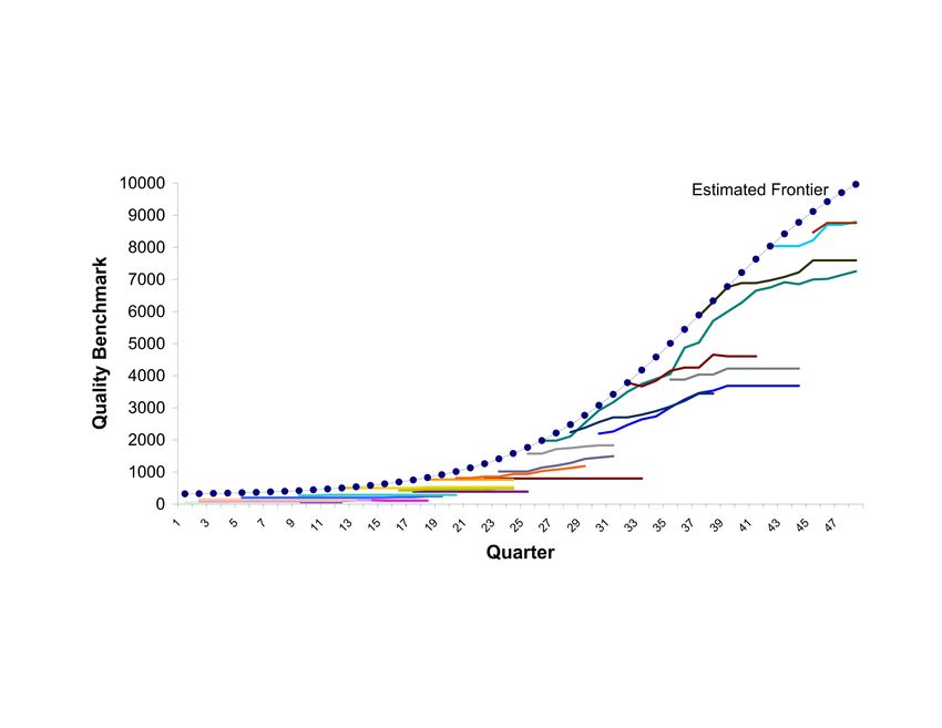
Figure 1 presents the observed evolution of quality of the products in
the dataset and the estimated quality frontier. The individuals colored lines
show the obsreved index of quality for a given product over its life and the
doted blue line shows the estimated logistic quality frontier.
5.3 Policy function
I estimate the policy function using a quadratic polynomial approximation.
Prices are predicted using pro
t-relevant state variables as explanatory vari-
albes. The variables used to predict product prices are the relative quality of
the good compared to the quality of the best product available in the mar-
28Figure 1: Evolution of Quality and Quality Frontier
ket (which enters the demand function) the production experience (which
determines production costs) and the total experience of the competitor
(which captures the eect of a
rm' choices over the competitor response
in the MPE). Figure 2 shows the observed and predicted prices using the
estimated quadratic approximation to the policy function. The dierences
between observed and predicted are assumed to be the realized cost shocks.
5.4 Cost Parameters
I estimate two models of the cost function. In the
rst model I assume that
the cost function is common to both
rms. Firms face the same cost func-
tion, but they have dierent costs because they have products with dierent
characteristics (die size and number of transistors) and dierent production
29Figure 2: Policy Function
levels, and therefore are at dierent locations along the learning curve. In
the second model, I incorporate a dummy variable for AMD to control for
other potential cost dierences between the two
rms. The estimated cost
parameters are presented in Table 5. All of the parameters are statistically
signi
cant at a 5% con
dence level, except for the die size, which becomes
insigni
cant in Model 2.
The Table 6 shows estimated average learning rates and average cost for
each time period, for each
rm, and for both cost models. Learning rates
uctuate between 2.54% and 24.86%. On average, Model 1 yields higher
learning rates, with an average of 11.46% for AMD and 14.40% for Intel.
Model 2 yields lower learning rates, with an average of 3.33% for AMD and
8.07% for Intel. Also, in Model 2 AMD's average costs is more than twice
the average cost of Intel, while in Model 1 AMD's average cost is just 23.5%
30Table 5: Estimated Cost Parameters
Model 1
Var. Coe. St. Error t-value p-value
Constant 142.6800 11.8530 12.0375 0.0000
Die Size 0.0758 0.0270 2.8027 0.0082
Transistors 0.2564 0.0609 4.2118 0.0000
Experience 10.7329 0.8126 13.2077 0.0000
Model 2
Var. Coe. St. Error t-value p-value
Constant 49.9756 0.9564 52.25 0.0000
Die Size 0.0602 0.1390 0.43 0.3633
Transistors 0.2607 0.0670 3.89 0.0002
Experience 4.5174 0.4199 10.76 0.0000
Dummy AMD 49.2492 0.3593 137.07 0.0000
higher than Intel's cost. The dierences in cost between
rms in Model 2
are explained mostly (88%) by the constant term and the remaining 12% is
explained by lower learning due to lower production volumes by AMD.
6 Conclusions
In this paper I have estimated a dynamic cost function with learning-by-
doing in the PC CPU industry. The results shows that there exists impor-
tant dierences in
rms' estimated production costs, with AMD's average
costs being more than twice Intel's average costs in a model in which the cost
function is allowed to dier between
rms. These dierences in production
costs are explained by both higher production costs when products are intro-
duced, as well as lower learning due to lower production volumes by AMD.
The average estimated learning rates
uctuate between 2.18% and 22.01%.
These rates are lower when compared to previous studies for other semicon-
31Table 6: Average Learning Rates and Production Costs by Firm
Model 1 Model 2
Learning Rates Prouduction Costs Learning Rates Prouduction Costs
Quarter AMD INTEL AMD INTEL AMD INTEL AMD INTEL
1 5.00% 4.99% 148.89 149.06 2.72% 4.74% 115.14 66.1
2 10.93% 5.37% 68.06 138.44 3.66% 4.98% 85.6 62.84
3 10.12% 11.27% 73.51 66.03 3.57% 8.70% 87.62 35.99
4 9.21% 12.98% 80.77 57.32 3.47% 9.39% 90.31 33.35
5 9.82% 12.83% 75.79 58 3.54% 9.44% 88.5 33.16
6 10.75% 12.60% 69.21 59.05 3.64% 8.51% 86.1 36.77
7 11.70% 12.54% 63.58 59.34 3.73% 8.17% 84.05 38.31
8 12.32% 11.59% 60.4 64.2 3.78% 7.50% 82.9 41.77
9 13.22% 11.99% 56.28 62.05 3.85% 7.75% 81.39 40.4
10 14.04% 11.78% 52.99 63.14 3.90% 8.26% 80.19 37.89
11 14.79% 12.64% 50.29 58.84 3.95% 8.65% 79.21 36.2
12 15.40% 13.69% 48.3 54.36 3.99% 9.06% 78.48 34.55
13 16.01% 14.03% 46.46 53.02 4.02% 9.22% 77.81 33.98
14 16.50% 14.33% 45.08 51.91 4.05% 8.66% 77.33 36.16
15 16.91% 16.95% 44 43.89 4.07% 9.90% 76.99 31.64
16 17.11% 13.78% 43.48 53.97 4.07% 8.50% 76.94 36.82
17 9.73% 12.87% 76.46 57.8 3.29% 7.35% 95.06 42.6
18 5.71% 11.54% 130.27 64.45 2.54% 6.63% 123.28 47.21
19 7.91% 10.84% 94 68.63 2.84% 5.62% 110.21 55.69
20 9.33% 10.27% 79.77 72.42 2.98% 5.37% 105.01 58.29
21 10.36% 9.35% 71.79 79.57 3.07% 6.21% 102.09 50.44
22 10.83% 11.82% 68.69 62.94 3.11% 7.11% 100.84 44.04
23 8.88% 14.40% 83.82 51.65 3.13% 7.81% 100.14 40.09
24 11.22% 17.27% 66.3 43.07 3.37% 8.53% 92.97 36.72
25 13.10% 13.80% 56.8 53.91 3.51% 7.71% 89.32 40.63
26 13.42% 14.65% 55.44 50.78 3.52% 7.94% 88.86 39.46
27 6.76% 14.74% 110.02 50.48 2.77% 7.96% 113.02 39.33
28 9.61% 10.26% 77.38 72.5 3.12% 6.79% 100.27 46.09
29 9.59% 13.62% 77.56 54.6 3.08% 8.68% 101.65 36.06
30 10.24% 17.68% 72.62 42.07 3.13% 9.98% 100.12 31.36
31 10.95% 21.74% 67.94 34.23 3.18% 10.99% 98.4 28.48
32 11.73% 24.86% 63.45 29.93 3.24% 11.61% 96.6 26.98
33 12.04% 22.64% 61.77 32.86 3.25% 10.41% 96.3 30.08
34 12.08% 24.41% 61.59 30.48 3.24% 10.58% 96.6 29.61
35 12.78% 20.97% 58.23 35.47 3.32% 9.87% 94.18 31.73
36 13.39% 21.28% 55.58 34.95 3.37% 10.04% 93 31.2
37 13.85% 15.35% 53.7 48.46 3.37% 8.76% 92.89 35.72
38 14.28% 11.72% 52.09 63.47 3.37% 7.22% 92.92 43.4
39 14.46% 15.08% 51.44 49.34 3.36% 8.24% 93.13 38.01
40 14.63% 14.37% 50.87 51.79 3.36% 7.16% 93.09 43.73
41 15.07% 16.17% 49.36 46 3.39% 7.53% 92.4 41.58
42 14.73% 16.97% 50.51 43.84 3.37% 7.30% 92.99 42.89
43 9.30% 18.09% 80.02 41.13 2.93% 7.32% 106.96 42.77
44 7.48% 19.35% 99.49 38.44 2.67% 7.47% 117.39 41.92
45 7.35% 13.84% 101.28 53.74 2.62% 6.70% 119.55 46.73
46 7.85% 11.55% 94.82 64.4 2.66% 6.55% 117.64 47.82
47 8.81% 12.16% 84.43 61.17 2.77% 6.89% 113 45.47
48 8.62% 13.98% 86.33 53.23 2.73% 7.49% 114.8 41.82
Min 5.00% 4.99% 43.48 29.93 2.54% 4.74% 76.94 26.98
Average 11.46% 14.40% 70.23 56.88 3.33% 8.07% 95.69 40.29
Max 17.11% 24.86% 148.89 149.06 4.07% 11.61% 123.28 66.1
32ductor products that have found average learning rates around 20%. This is
an indication that
rms are more successful in transfering the products from
the development to fabrication facilities and have already advanced in their
learning curve when the products are introduced into the market. Neverthe-
less, given the importance of CPU products for the industry this result is
not surprising.
33References
[1] Aizcorbe, A. (2005) Moore's Law and the Semiconductor Industry: A
Vintage Model, Scandinavian Journal of Economics, Vol. 107(4), pp.
603-630.
[2] Aizcorbe, A. (2006) Why Did Semiconductor Price Indexes Fall So Fast
in the 1990s? A Decomposition Economic Inquiry, Volume 44 (3) pp.
485-496.
[3] Bajari Patrick, Leniard Benkard and Jonathan Levin. 2007 Estimating
Dynamic Models of Imperfect Competition, Econometrica, Vol. 75 (5),
pp. 1331-1370.
[4] Baldwin and Krugman (1988), Market Access and International Com-
petition: A Simulation Study of 16K RAM. In Feenstra (ed.) Empirical
Methods for International Trade, MIT Press, Cambridge, MA.
[5] Berry, S., J. Levinsohn and A. Pakes (1995). Automobile Prices in Mar-
ket Equilibrium, Econometrica, 63, 841-890.
[6] Besanko, D., U. Doraszelski and Y. Kryukov (2007) Learning-by-Doing,
Organizational Forgetting and Industry Dynamics, Unpublished work-
ing paper, Kellog School of Management, Northwestern University.
[7] Cabral, R. and M. Leiblein (2001) Adoption of a Process Innovation
with Learning-by-doing: Evidence from the Semiconductor Industry
The Journal of Industrial Economics Vol XLIX (3), pp. 269-280.
34[8] Cabral, L. and M. Riordan (1994), The Learning Curve, Market Domi-
nance and Predatory Pricing, Econometrica, Vol. 62 (5), pp. 1115-1140.
[9] Dasgupta, P., AND J. Stiglitz (1988): "Learning-by-Doing, Market
Structure and Industrial and Trade Policies," Oxford Economic Papers
Vol. 40, pp. 246-268.
[10] Dick, J. (1991) Learning by Doing and Dumping in the Semiconductor
Industry, Journal of Law and Economics, Vol. 34 (1), pp. 133-159.
[11] Fourer, R., D. Gay and B. Kernighan (2002) AMPL: A Modeling Lan-
guage for Mathematical Programming, Duxbury Press, 2nd Edition.
[12] Fudenberg, D., AND J. Tirole (1983):" Learning-by-Doing d Market
Performance," Bell Journal of Economics, 14, 522-530.
[13] Ghemawat, P. and Spence, M. (1985), Learning curve spillovers and
market performance, Quarterly Journal of Economics 100, pp. 839-852.
[14] Gilbert, R. and G. Harris (1981), Investment Decisions with Economies
of Scale and Learning, American Economic Review, Papers and Proceed-
ings, Vol. 71, 172-177.
[15] Gordon, B. (2008). A Dynamic Model of Consumer Replacement Cycles
in the PC Processor Industry Unpublished working paper, Columbia
Business School, January 2008.
[16] Gruber, H. (1992) Persistence of Leadership in Product Innovation,
Journal of Industrial Economics, 40, pp. 359-375.
35[17] Gruber, H. (1996) Trade Policy and Learning by doing: The case of
semiconductors Research Policy Vol. 25, pp. 723-739.
[18] Gruber, H. (1998) Learning by Doing and Spillovers: Further Evidence
for the Semiconductor Industry. Review of Industrial Organization Vol.
13, pp. 697-711.
[19] Habermeier, K. (1992): The Learning Curve and Competition, Inter-
national Journal of Industrial Organization Vol. 10, pp. 369-392.
[20] Hatch, N. 1996. Enhancing the Rate of Learning by Doing Through Hu-
man Resource Management. In THE COMPETITIVE SEMICONDUC-
TOR MANUFACTURING HUMAN RESOURCES PROJECT : Second
Interim Report CSM-32. Clair Brown, Editor. Institute of Industrial Re-
lations, University of California at Berkeley.
[21] Hatch, N. and Reichelstein. 1994. Learning eects in semiconductor
fabrication. Competitive Semiconductor Manufacturing Program Report
CSM-33, University of California at Berkeley.
[22] Hatch, N. and D. Mowery. 1998. Process Innovation and learning-by-
doing in Semiconductor Manufacturing. Management Science, Vol 44,
N. 11.
[23] Irwin, D. and P. Klenow. 1994. Learning-by-Doing Spillovers in the
Semiconductor Industry. The Journal of Political Economy Vol. 102 (6),
pp. 1200-1227.
36[24] Lee, W. (1975), Oligopoly and Entry Journal of Economic Theory,
Vol. 11, pp. 35-54.
[25] Mookherjee, D. and D. Ray (1991), Collusive Market Structure under
Learning-by-Doing and Increasing Returns," emphReview of Economic
Studies Vol. 58, pp. 993-1009.
[26] Macher, J. and D. Mowery (2003) Managing Learning-by-Doing: An
Empirical Study in Semiconductor Manufacturing The Journal of Prod-
uct Innovation Management, Vol 20, pp. 391-410.
[27] Nevo, A. (2000), A Practitioner's Guide to Estimation of Random-
Coe
cients Logit Models of Demand, Journal of Economics and Man-
agement Strategy, Vol. 9, No.4, 513-548.
[28] Ross, D. (1986), "Learning to Dominate," Journal of Industrial Eco-
nomics Vol. 34, pp. 337-353.
[29] Salgado, H. (2008), Brand Loyalty, Advertising and Demand for Com-
puter Processors: The Intel Inside R Eect. Unpublished Working Pa-
per, Department of Agricultural and Resource Economics, University of
California at Berkeley.
[30] Siebert, R. (2008), Learning-by-doing and Multiproduction Eects
through Product Dierentiation: Evidence from the Semiconductor In-
dustry. Unpublished working paper.
37[31] Song, M. (2007) Measuring Consumer Welfare in the CPU Market: An
Application of the Pure Characteristics Demand Model RAND Journal
of Economics, Vol. 38, pp. 429-446.
[32] Spence, M. (1981), The learning curve and competition, Bell Journal
of Economics Vol. 12(1), pp. 49-70.
[33] Wright, T. (1936) Factors Aecting the Cost of Airplanes, Journal of
Aeronautical Science Vol 3(4), pp. 122-128.
38You can also read