Testing marine data assimilation in the northeastern Baltic using satellite SST products from the Copernicus Marine Environment Monitoring Service ...
←
→
Page content transcription
If your browser does not render page correctly, please read the page content below
Proceedings of the Estonian Academy of Sciences, 2018, 67, 3,

                                  Proceedings of the Estonian Academy of Sciences,
                                                2018, 67, 3, 217–230
                                            https://doi.org/10.3176/proc.2018.3.03
                                          Available online at www.eap.ee/proceedings

Testing marine data assimilation in the northeastern Baltic using satellite
  SST products from the Copernicus Marine Environment Monitoring
                                 Service
                                            Mihhail Zujev* and Jüri Elken
Department of Marine Systems, Tallinn University of Technology, Akadeemia tee 15A, 12618 Tallinn, Estonia

Received 14 August 2017, accepted 2 January 2018, available online 5 June 2018

© 2018 Authors. This is an Open Access article distributed under the terms and conditions of the Creative Commons Attribution-
NonCommercial 4.0 International License (http://creativecommons.org/licenses/by-nc/4.0/).

Abstract. Satellite SST products from the Copernicus Marine Environment Service were tested for data assimilation in the
sub-regional marine forecasts. The sub-regional setup of the HBM model was used in the northeastern Baltic, covering also
the Gulf of Finland and the Gulf of Riga. Two assimilation methods – successive corrections and optimal interpolation – were
implemented on the daily forecasts from April to December 2015. Independent daily FerryBox data from the ship track between
Tallinn and Helsinki were used for validation. Higher SST forecast errors of the reference model were found near the shallower
northwestern coasts. During the calm heating period in spring and early summer, the reference model produced in these regions
too warm waters compared with the satellite and FerryBox observations. Too cold waters, compared to the observations, were
modelled during the cooling period from late summer to winter. Although data assimilation reduced these errors, improving the
treatment of coastal–offshore exchange in the core forecast model would be useful.

Key words: remote sensing, data assimilation, successive corrections, optimal interpolation, short-term forecast, HBM model,
SST assimilation.

1. INTRODUCTION                                                  been made. Shipborne observations, which provide most
*
                                                                 of the water column data, are non-synoptic and usually
Assimilation of observational results into oceanographic         separated by a distance larger than the scale (size)
forecast models has a history of several decades,                of mesoscale motions. About a decade later than in
following with some delay developments of data                   meteorology, the first global oceanic data assimilation
assimilation in meteorology. In parallel to statistical          system (Derber and Rosati, 1989) was proposed based
forecast correction methods based on linear filtering            on sea surface temperature (SST) observations from
and prediction theories (e.g. Kalman and Bucy, 1961),            merchant ships; quite sparse profile data from XBT, CTD,
Cressman (1959) proposed a robust ‘manually tunable’             and Nansen bottles were incorporated as well.
method directly applicable for correcting weather                    Acquisition and assimilation of remote sensing data
forecasts. Meteorology reached the state of working              have been a common procedure for both meteorology
operational assimilation and forecast systems already in         and oceanography. However, the data coverage and
the 1970s (McPherson et al., 1979). In oceanography,             accuracy are different for the atmosphere and the ocean.
only a few offshore regular time series observations have        Reliable spaceborne thermal emissivity observations
                                                                 started in the 1960s on terrestrial (Buettner and Kern,
*
    Corresponding author, mihhail.zujev@ttu.ee                   1965) and ocean (Anding and Kauth, 1970) surfaces.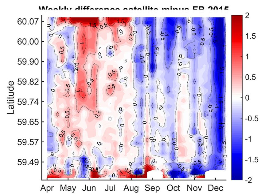
218                                                   Proceedings of the Estonian Academy of Sciences, 2018, 67, 3, 217–230

Further, atmospheric infrared and microwave sounding           ponding perturbations propagate much slower as
allowed estimation of temperature and humidity profiles        baroclinic internal waves or advective plumes; hence
with height, also in the cloudy areas. Operational             larger innovations are acceptable. When observations
assimilation of remote sensing data into the weather           of different state variables are combined into the same
forecast models was introduced in the 1970s, based on          forecast, multivariate optimal interpolation provides
the adding of interpolated difference between observed         reliable results (Cummings, 2005).
and forecast values to the original forecast in order to           In the Baltic Sea, probably the first data assimilation
obtain a corrected model state for the next forecast           system was made by Sokolov et al. (1997) for ‘smart’
interval. The tests showed (e.g. Ghil et al., 1979) that       interpolation of temperature, salinity, and chemical profile
the impact of data assimilation is highly sensitive to the     data from monitoring stations, using a hydrodynamic
quantity of data available; the choice of the assimilation     model. Some tests have been devoted to assimilation
method to determine the interpolation weights is also of       of sea level data (Canizares et al., 2001; Sørensen and
importance.                                                    Madsen, 2004; Ivanov et al., 2012), based on the various
    Ocean sea surface temperature (SST) can be                 options of the Kalman filter.
determined by most satellite sensors only in the cloud-            Assimilation of scalar variables such as temperature
free areas. Again, the amount of ocean data on the             and salinity into the Baltic Sea models has a quite rich
surface is irregular both in time and space as these are       history. The present study has some specific features.
temperature–depth profile data; this causes significant        Firstly, assimilation is designed into the operational
problems in ocean data assimilation, compared with the         forecast system and is prepared for the routine use;
more regular atmospheric observational data. Skin-layer        therefore, the methods must be robust and computatio-
corrected accurate (Donlon et al., 2002) and operationally     nally effective. Secondly, the study is based on the
available SST data that have high resolution both in           downstream forecasts from the Baltic-wide core service
space (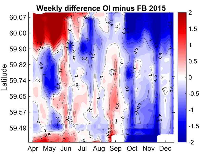
M. Zujev and J. Elken: Testing marine data assimilation in the northeastern Baltic 219
assimilation. We discuss possible ways to use less miles is further refined into a 1-mile grid covering the
costly assimilation methods, yielding the results of nearly whole Baltic Sea. In the Danish Straits, two-way nesting
the same quality as with more sophisticated methods. with a finer grid model with the resolution of 0.5 nautical
Finally, conclusions are presented. miles is used.
The Estonian implementation of the HBM (Lagemaa,
2012) covers the Baltic Sea sub-area east from 21.55°E
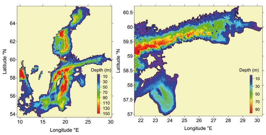
2. MODEL, DATA, AND METHODS (Fig. 1), including the Gulf of Finland and the Gulf of
2.1. Sub-regional marine forecast model HBM Riga, with the resolution of 0.5 nautical miles. The
horizontal grid of the HBM-EST model consists of 425
For assimilation tests we used the HBM-EST model by 529 grid points. The grid cell length by longitude
(Lagemaa, 2012), which is an Estonian implementation is 1′, by latitude it is 30″. In the vertical grid, 39 depth
of the HBM model (the abbreviation comes from layers are used, with a 3-m grid step near the surface
HIROMB-BOOS Model). The model was originally and larger grid steps in the deeper layers. Forcing at
constructed by the Bundesamt für Seeschifffahrt und the western open boundary is taken from the Baltic-
Hydrographie, Hamburg, Germany, named as BSHCmod. wide HBM model, which operates routinely within the
Further developments have been made within Baltic- CMEMS with the resolution of 1 nautical mile. Forcing
wide cooperation in operational forecasting; different on the sea surface is obtained from the Estonian version
options were merged to a new thoroughly tested HBM of the HIRLAM model that is run by the national weather
code within the EU MyOcean project. Details of the service for operational forecasts on a 11-km grid. For
HBM model and its implementation are given by Berg analysis of observation and forecast errors in relation to
and Poulsen (2012). wind conditions, time series of wind speed components
The HBM is a free-surface baroclinic 3D ocean were extracted in the central part of the Gulf of Finland.
model written in geographical latitude/longitude spherical We chose the year 2015 for the forecasting and
coordinates that uses a horizontal staggered Arakawa assimilation experiment. The forecasts were updated
C-grid and a fixed vertical grid with variable spacing daily by introducing a new weather forecast at midnight.
and time-varying top layer thickness. There is also
an option for dynamical vertical coordinates where 2.2. Satellite SST data
the grid spacing changes in time. Vertical turbulence
is treated by the – turbulence model and horizontal Sea surface temperature data, observed from satellites,
turbulence is treated within the well-known Smagorinsky were used as input observational data within data
formulation. The sea ice module is an integrated part assimilation. Gridded observation maps were obtained
of the HBM model, including both dynamics and from the CMEMS multi-sensor product, which is built
thermodynamics. The model can take into account the from bias-corrected L3 mono-sensor products at the
results from independent wave models. horizontal resolution of 0.02 by 0.02 degrees. For each
The forcing of the model is done by externally day a single SST value was used, which was reduced
prescribed surface fields, point sources, and open to midnight based on available observations at different
boundary conditions. Surface fields are adopted from times (near-real-time).
the numerical weather prediction model: 10-m wind This product (Bonekamp et al., 2016) contains results
components, mean sea level atmospheric pressure, from the merging of various satellite SST level 2 data,
surface air temperature, surface air humidity, and cloud which have passed a significant number of quality controls
cover. The HBM model calculates surface energy fluxes and which have been calibrated through an inter-sensor
(mechanical, radiative, thermodynamic) using bulk bias correction procedure to provide an estimate of the
parameterization formulae. Point source data are night time SST based on original SST observations
freshwater fluxes from rivers. If actual discharge without any smoothing or interpolation. Details of
forecasts are missing, the climatology for each calendar the product are described on CMEMS web resource
day will be used. http://cmems-resources.cls.fr/documents/QUID/CMEMS-
On the ocean side, the HBM model is forced by the OSI-QUID-010-009-a.pdf.
tidal sea surface elevation, sea level forecasts from the Sensors used include METOP_B, SEVIRI,
barotropic storm surge model of the Northern Atlantic, VIIRS_NPP, MODIS, and others. Observations were
and monthly climatological hydrography. The Baltic Sea collected from different producers: NASA, NOAA,
implementation of the HBM uses a nested approach: the IFREMER, EUMETSAT OSI-SAF, and ESA.
largest area of the 3D forecast covers the North and Depending on the cloud cover there were from 200
Baltic seas with a grid step of 12 nautical miles, the up to 21 000 observations per day. Some obviously
intermediate resolution with a grid step of 3 nautical erroneous SST values (which differed more than 10 K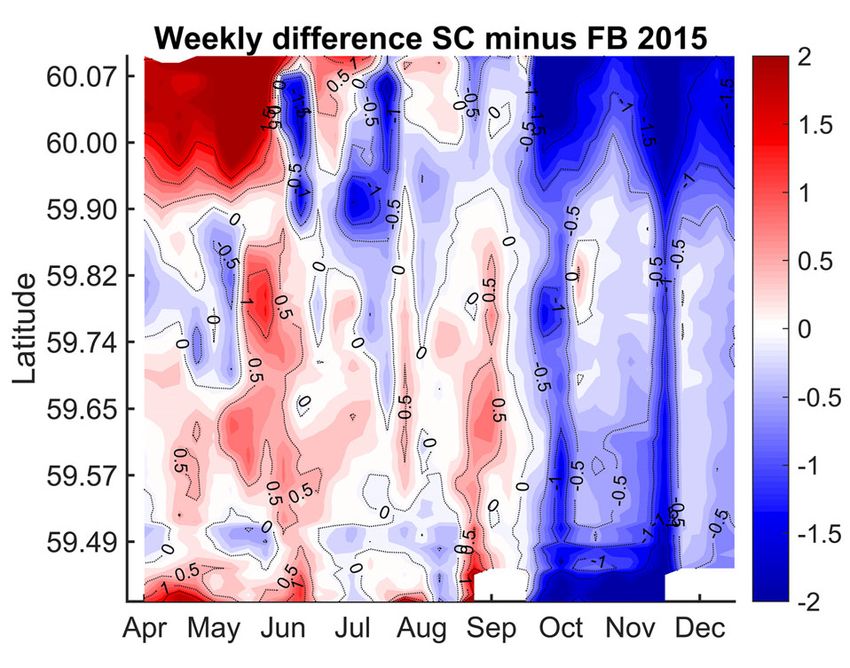
220 Proceedings of the Estonian Academy of Sciences, 2018, 67, 3, 217–230
from model ones) were filtered out. All of them were are taken usually at different n locations than x b .
used for the assimilation with the Cressman method. For Assimilation is a procedure to create the analysis vector
optimal interpolation a data thinning algorithm was x a on the same set of coordinates as x b with a
implemented, leaving one value for the area of 2.5 by 5 condition that by a given set of criteria, x a is closer
nautical miles. to y than x b . When the model state values ŷ in the
An example of data extracts is shown in Fig. 2a, points of observations are obtained by an interpolation
representing the observations on the line between procedure, then the analysis is calculated from the
Tallinn and Helsinki during the whole test period. innovation vector y yˆ by the formula
The temperatures presented here are averaged over one
week. x a x b K ( y yˆ ) , (1)
where K is the gain matrix containing m n weights
2.3. FerryBox data
for interpolation over 1 n observation points. At
individual model grid point i formula (1) can be written
Automatic observations made from ships crossing the
using the weight vector w i K i . In the following
sea areas were used as independent data for validation
formulae we consider one state variable only and omit
and quality assessment. FerryBox is a measurement
the index i , describing the specific model grid point.
system installed on board commercial ferries that collects
As a result we obtain
temperature, salinity, chlorophyll a fluorescence, and
n
turbidity data. This technology is used to study basin-
scale temperature and salinity patterns together with
xa xb w y ŷ xb w y yˆ .
j 1
j j j (2)
mesoscale processes and upwellings (Kikas and Lips,
2016). The water is sampled at about 4 m below the 2.4.1. Successive corrections
surface at different rates and every 20 s the measure-
ment is recorded, thus covering roughly 160–200 m The successive correction method or the Cressman
in the horizontal direction. There are quality check (1959) method assumes univariate relations between
procedures to eliminate unexpected and physically un- the state variables and that weights of the individual
realistic values; cross-checking with the same data from observations w j in (2) decrease with the distance d j
the return trip is performed as well (Kikas and Lips, between the observation point j and the model grid
2016). Detailed description of technical features of the point i . Let us define the influence radius R around
FerryBox system is given by Lips et al. (2008). the model point i , where k observations out of total n
Observations are available on the route Tallinn– observations are located. Good assimilation results are
Helsinki on the forth and back tracks twice a day with obtained with the weights given by the formula
a time step of 20 s. Temperatures on the same latitude
were averaged across multiple tracks. For each day one R 2 d 2j
max 0, 2 2
mean SST value was calculated regardless of the time of R dj
the day and the number of observations in the particular wj , (3)
n R 2 d 2j 2
grid cell. Weekly averages of the temperatures observed max 0, 2 2
by the FerryBox system are shown in Fig. 2b. j 1 R dj
The data were taken as they are within the Copernicus
where the weights are positive within the influence
system, in which the procedures include an advanced
radius and zero elsewhere. Reduction of the assimilation
quality check. As our aim was to check the working
weights in real noisy conditions is done by introducing
of automatic systems, no additional quality control or
relative noise variance 2 , estimated from the variances
processing was performed.
of observation errors o2 and background errors b2 ,
2 o2 b2 . In the noiseless case ( 2 = 0) the sum of
2.4. Data assimilation weights is equal to unity.
Data assimilation for SST was made using a medium-
Let us consider the model state represented by a vector scale value 37 km (20 nautical miles, 40 grid points)
x u, v, T , S , , ,... , where the values in brackets for the influence radius. This length is about ten times
are the model state variables (velocity components, larger than the Rossby deformation radius. Therefore,
temperature, salinity, water density, sea level, etc.), the impact of individual mesoscale eddies is suppressed,
generally given at discrete grid points. When the model but basin-scale SST features are kept. The weight
predicts the state vector x b on m grid points, it has function has the greatest impact within the nearest 5 km,
some errors regarding the true state. Observations y then it goes almost linearly to zero for 37 km. Before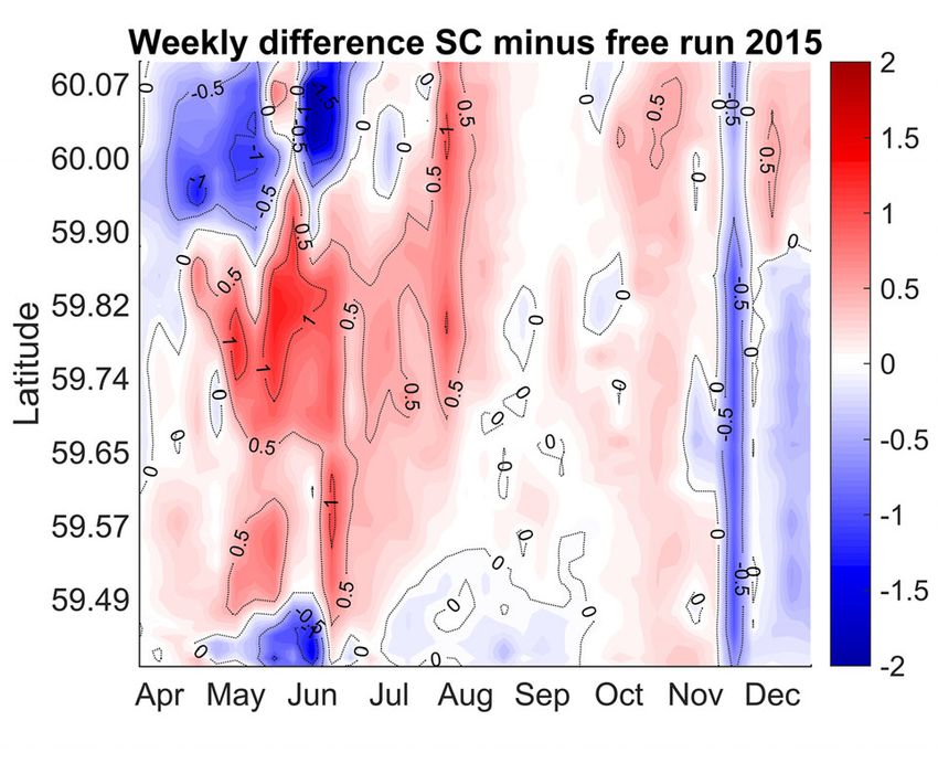
M. Zujev and J. Elken: Testing marine data assimilation in the northeastern Baltic                                           221

           (a)                                               (b)

           (c)

                                                                            Fig. 1. Map of the HBM-EST model domain
                                                                            with depth contours (b) and its location on
                                                                            the map of the Baltic (a). Panel (c) shows the
                                                                            observation points along the FerryBox track
                                                                            used for validation.

     (a)                                                              (b)
                 Weekly satellite observations 2015                                  Weekly FerryBox data 2015

Fig. 2. Time–latitude map of the weekly mean sea surface temperature observed from satellites (a) and FerryBox (b) between
Tallinn (south) and Helsinki (north).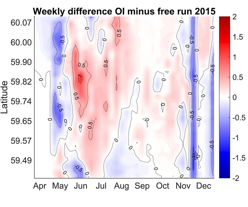
222 Proceedings of the Estonian Academy of Sciences, 2018, 67, 3, 217–230
assimilation, the observations were averaged over each the background field (Lorenc, 1986; Ide et al., 1997).
grid cell in order to avoid oversampling problems. However, most of the practical implementations, like in
During the testing of the scheme, the values of o2 and our case, are limited to equations (4) with solution (5),
b2 were not known in advance. For the chosen data set where the spatial correlation is prescribed as a function
we obtained acceptable results with R = 37 km and with ‘tuned’ parameters.
2 o2 b2 = 2. We used these values throughout the Correlations B and b were approximated by the
entire model run. Gaussian function from the distance r between the
For computational efficiency, assimilation was correlated points. Anisotropic correlation features were
performed in the two-dimensional domain for the surface taken into account by the directional distribution of
layer only; deeper model levels were left unaffected. the correlation scale from the angle in the form of
Since the observations were assimilated every day, the the ellipse dependence L a sin 0 b cos 0
introduced innovations were moderate (compared to the relative to the reference angle 0 . So the correlation
vertical mixing) and not visible in the graphs of vertical
was adopted in the form B r, exp r 2 L2 ,
profiles. where L L was pre-calculated in each model
grid point according to the coastline and topography.
2.4.2. Optimal interpolation Following the results by Høyer and She (2007), longer
correlation scales were adopted along the coasts and the
Optimal interpolation as developed by Gandin (1963)
isobaths than in the perpendicular direction. The typical
uses least-square minimization of analysis errors to
horizontal impact scale along the coast or isobath was
calculate the weight coefficients w j in expression (2).
chosen as 15 km. Standard deviations for the entire run
We follow the original point-wise presentation (see
were taken o2 = 0.5 and m2 = 1.0.
also Høyer and She, 2007) and denote f j y j yˆ j ,
Before performing the assimilation according to
f0 ~
xa xb . Here ~
x a is the ‘true’ unknown state in
equations (2) and (5), the observations were filtered with
the model point i . The observations include random
a thinning algorithm to avoid oversampling and a huge
errors j ; the error variance is 2j . The squared
computation amount, leaving up to n = 700 points. The
interpolation error, averaged over an ensemble,
distance between the generated super-observations was
2
n kept at 10 km or more. For computational efficiency,
E f0
w j f j j min is minimized with
wet points (located in the sea) were divided into 30
j 1 blocks to cover the entire basin. That leaves up to 81
respect to w j . This is achieved by setting n constraints observations per block. Observations from each block
for the derivatives E w j 0 , using the conditions were cross-compared with all other observations in the
f j 0 , f 0 0 , j 0 , j f j 0 , j f 0 0 . As a same block plus the neighbouring observations falling
result, we obtain for the ith model point the following into the adjacent area within a radius of 100 km, and the
system of n linear equations regarding w j : correlation coefficients were calculated.
n
f
j 1
k f j w j 2k w j f k f 0 , k 1 ... n , (4)
2.5. Methods for data quality and model skill
assessments
which can be easily solved. By dividing equations (4)
by the variance 2f f k2 , we obtain correlation instead There are a number of different SST data sets that can
of spatial covariance. The weight coefficients of optimal be compared. Here remote sensing SST products (SAT)
interpolation are determined by the correlation matrix from CMEMS are used for data assimilation. FerryBox
between the individual observation points B f k f j 2f observations (FB), carried out by the Department of
and the correlation vector between the observation point Marine Systems but accessed from the Copernicus
and the ith model point b f k f 0 2f , and by the service, provide independent data for the assessment of
relative variance of observation error 2 2k 2f . the skill of data assimilation. Before estimating the skill
Equation (4) can be rewritten as w B 2 I b , where of model versions (without data assimilation or with
I is a unit matrix. The vector of weights is calculated in different assimilation options) in reference to one or
the form another observational data set, the observations from
w b B 2I 1
. (5) different platforms are compared.
Following the approach by Taylor (2001), for each
More general matrix-vector formulations of optimal comparison of the two variables f n and gn a common
interpolation can handle also the case where observation data set is defined where missing values of one or both
errors may be correlated between each other and with data sets are ignored. If the standard deviations of the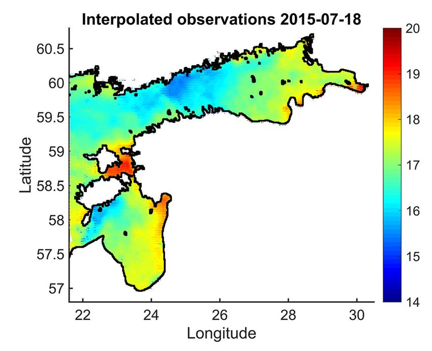
M. Zujev and J. Elken: Testing marine data assimilation in the northeastern Baltic 223
data sets are f , g and the coefficient of their mutual Weekly difference satellite minus FB 2015
correlation is R f , g , then the centred (with bias removed)
root-mean-squared difference (RMSD) of the data sets
E will read
E 2 2f g2 2 f g R f , g . (6)
The size of the original data sets is very different.
Therefore we reduced in many cases the compared data
sets to the FerryBox transect between Tallinn and
Helsinki. Such data form a time–latitude matrix with
a daily step in time and a 2.222 km step by latitude.
For the data gap treatment we used the weekly average
of all the available data. The missing values were just
omitted from the averaging. Since satellite data were
recalculated to the midnight values, for this comparison Fig. 3. Weekly mean sea surface temperature difference
between the satellite and FerryBox observations on a transect
the forecast was treated as the weekly average of nightly
between Tallinn (south) and Helsinki (north) as a function of
(23 h advance) values. Other data set definitions are time and latitude.
explained in the results section when necessary.
The model data sets are named as FR (‘free’ model
run without data assimilation), SC (model run with upper layer (observed at 4 m depth) during spring and
assimilation of Copernicus SST with successive correction summer until August but insignificantly (less than 0.5 K)
method), and OI (model run with assimilation of smaller in autumn and early winter. Larger SAT minus
Copernicus SST with the optimal interpolation method). FB differences emerged occasionally in areas close
The model data sets have 71986 values for each time step. to the coasts: a range 0.7–1.0 K was observed in Tallinn
Bay and a larger range, 1.0–2.5 K, was found near
Helsinki. In December the thin surface layer cooled
3. RESULTS down by 0.5–1.5 K more than the deeper surface layer
3.1. Comparison of SST from satellite and along the whole transect, including also the coastal waters.
FerryBox In most of the cases the difference between the two
data sets (SAT minus FB) was of the same sign over the
There are principal differences between the temperature whole transect. This is consistent with the results by
observed from satellites and from in situ sensors located Uiboupin and Laanemets (2015), who studied similar
a few metres below the surface. These observations give data from 2000–2009. They found that during wind
closer results in well-mixed conditions (Siegel et al., speeds less than 5 m/s different satellite sensors give
2006; Uiboupin and Laanemets, 2015), which occur up to 3 K larger SST than it is observed by FB; the
during stronger winds. difference is largest at smaller wind speeds of 2 m/s and
Here we compare averaged satellite observations less during temporary stratification of the thin surface
from the Copernicus service (SAT) during 2015 along layer. In our case with CMEMS data the difference was
the FerryBox track with the in situ data of the latter larger near the coasts, but both the coastal areas usually
(FB). Temperature values were merged by latitude, appeared in the SAT data either warmer or colder than it
leaving out the impact of ship track variations. Several was found from the FB data. The reasons for large SST
values for the same bin were replaced by their mean. differences between satellite and in situ observations
The SAT data were provided as of midnight while the were discussed by Siegel et al. (2006). They also noted
FB observations were made at different times during a seasonal behaviour as it is evident from our data
a particular day. The FB data represent the average presented in Fig. 3.
temperature in the upper mixed layer, whose depth is
variable. The data sets are independent of each other 3.2. Spatial patterns of SST
and have their maxima in August.
The difference between the two SST data sets is Sea surface temperature patterns manifest a variety of
shown in Fig. 3. In central parts of the Gulf of Finland physical processes like different heating or cooling in
(latitudes 59.5–60 N) there is a clear seasonal behaviour. coastal versus offshore areas, coastal upwelling, thermal
The thin layer temperature registered by the satellite fronts between the water masses, and signatures of
was 0.3–0.7 K larger than the bulk temperature of the mesoscale eddies and filaments.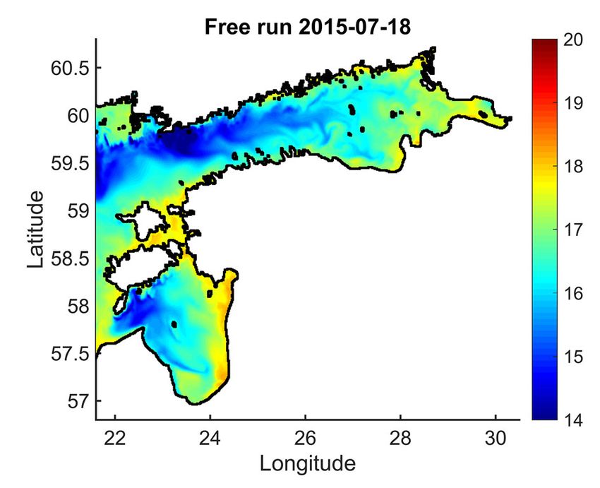
224                                                     Proceedings of the Estonian Academy of Sciences, 2018, 67, 3, 217–230

      (a)                                                                (b)
                     Free run 2015-07-18                                        Interpolated observations 2015-07-18

 Fig. 4. Example of a HBM forecast (a) and satellite observations interpolated on the same grid (b). Both data from 2015-07-18.

    We present an example of SST distributions for a              temperatures than FB during the warming period (see
summer date when there was good coverage of the sea               also Fig. 3). The SAT data were spiky compared with
area with satellite data. Comparison of the results of the        the FB data: warmer spikes occurred during the warming
model forecast (Fig. 4a) and remote sensing (Fig. 4b)             period and colder spikes during the cooling. The FR
reveals a different extent of warmer and colder areas of          forecast provided in the offshore waters slightly smaller
coastal waters. Model results show wide bands of colder           SST than observed. Data assimilation using SC and OI
water off the northern coasts, both in the Gulf of                ‘dragged’ the model results towards SAT observations,
Finland and the Gulf of Riga. Satellite data registered           still the SST spikes did not appear in the assimilated
only a small fraction of these colder water masses. In            model results.
the warmer shallow areas, located between the Estonian                 As the cross-gulf SST pattern (Fig. 5b) shows, the
larger islands and near the eastern coast of the Gulf of          southern part of the gulf warmed up faster than the
Riga, satellite observations yielded higher SST (by               central and northern parts, based on the results from SC-
about 1 K) than the model. This can be partly attributed          assimilated model data (see also weekly SAT and FB
also to the wind-dependent positive bias of satellite data        data in Fig. 2). This resulted in warmer by up to 5 K
(Uiboupin and Laanemets, 2015). We note that the                  waters on a specific day. Cooling took place more
model reproduces in the above example more distinct               uniformly across the research area, temperature differ-
mesoscale patterns than are evident from the satellite            ences were up to 1.5 K. Similar regional differences
data.                                                             were evident in other data sets.

3.3. Time series of SST                                           3.4. Skill assessment for non-assimilated and
                                                                       assimilated model results
In the adopted data assimilation approach, SST satellite
observations (example given in Fig. 4b) are used to               Independent FB data obtained in a cross-section of the
correct the model forecast (example given in Fig. 4a).            Gulf of Finland form the most comprehensive off-shore
FerryBox data are independent and intended for                    in situ data set within the forecast area. In the following
validation. The data as defined in Section 2 are from             we compare the assimilated model results obtained
observations (SAT and FB) and from models (FR, SC,                using the two methods with the FB data. For the non-
and OI). The data are compared on the FerryBox transect           assimilated model data (FR, reference run) we present
(see Fig. 1c), where all the data are available. The model        comparisons for model validation. Since the two
results are with a regular time interval (1 h), but daily         observations, SAT and FB, have different SST values
observations have gaps.                                           (see Section 3.1), comparison is also made in reference
    In the open part of the Gulf of Finland daily SAT             to remote sensing data that were used in the assimilation
data from CMEMS (Fig. 5a) revealed generally higher               process.
M. Zujev and J. Elken: Testing marine data assimilation in the northeastern Baltic 225
(a) (b)
Mean temperature in the open part in 2015 Mean temperature in the open part in 2015
(c)
SC in different regions of the Gulf of Finland in 2015
Fig. 5. Daily SST time series on the FerryBox transect in
the Gulf of Finland: (a) FB during the observation time
and nightly values for FR and SAT; (b) nightly values
for FR, SC, and OI, both (a) and (b) in the central part of
the transect; (c) nightly SC values in the northern, central,
and southern parts of the transect. For abbreviations,
see the title of Table 1.
Further we consider temporal evolution of cross-gulf observed during the periods of calmer winds in the
SST patterns in the Gulf of Finland on the basis of second half of May and August. Comparison of the
weekly average transects. Since the SAT data are results by SC and OI methods indicates that OI provided
from midnight, we used nightly model data for finding with a given set of parameters generally smaller differ-
the weekly averages. The difference between the daily ences from FB than SC, except in June and July near the
mean and nightly model values (not shown) due to the northern coast when OI produced larger differences than
diurnal cycle was up to 0.5 K from April to August and SC. We note that the SC method used the interpolation
slightly negative from September to December. weights not dependent on the direction between the
Both the SC and OI methods gave similar patterns of points; in case of OI longer correlation scales were used
differences relative to FB data (Fig. 6). These patterns along the coasts than in the cross-shore direction.
are similar to that of FR minus FB (not shown), but Within the data assimilation, greater changes in
the variations of difference have been reduced by the reference to FR (Fig. 7) were made by the OI than by
data assimilation. Greater differences were found in the the SC method. We selected the OI parameters on
northern part of the Gulf of Finland, where a positive the basis of some trials. However, investigation of the
difference was evident from April to August (although best combination of different parameters for OI is
the SC method gave some shorter negative differences outside the scope of this paper, reduction of sigma ratio
as well) and a negative difference from September to 2 o2 m2 by the factor of two did not yield plausible
December. In the central part of the gulf data assimilation results.
corrected the errors of FR effectively and the forecast Statistical comparison of weekly mean values of the
absolute difference from the FB data was in most cases FR forecast and the assimilated SC and OI forecasts
less than 0.5 K. Exceptions were found during stronger with FB data (Table 1) revealed that assimilation provided
winds at the beginning of October and November, when better correspondence to the independent observations.
the assimilated SST forecast remained by about 1 K Based on formula (6), improvements are visible in bias,
smaller than FB observations. Positive anomalies were RMSD, and correlation R. The main skill estimator –
226                                                      Proceedings of the Estonian Academy of Sciences, 2018, 67, 3, 217–230

      (a)                                                              (b)
             Weekly difference SC minus FB 2015                               Weekly difference OI minus FB 2015

Fig. 6. Time–latitude map of the weekly mean sea nightly surface temperature difference of assimilated with SC (a) and OI (b) in
reference to FerryBox data between Tallinn and Helsinki. For abbreviations, see the title of Table 1.

      (a)                                                               (b)
            Weekly difference SC minus free run 2015                          Weekly difference OI minus free run 2015

Fig. 7. Time–latitude map of the weekly mean nightly sea surface temperature difference of assimilated with SC (a) and OI (b) in
reference to non-assimilated model data between Tallinn and Helsinki. For abbreviations, see the title of Table 1.

      Table 1. Statistics of free model run without data assimilation (FR), model run with assimilation with the successive
      correction method (SC), model run with assimilation of Copernicus SST with the optimal interpolation method (OI),
      and remote sensing SST data (SAT) with reference to FerryBox data (FB)

                                            FR                SC                OI               SAT              FB
      Bias                               –0.45               –0.34             –0.42            –0.31            0
      RMSD                                0.97                0.84              0.96             0.66            0
      Correlation R                       0.931               0.937             0.934            0.936           1.00
      Mean                               10.99               11.11             11.03            11.13           11.45
      Standard deviation σ                4.35                4.45              4.48             4.57            4.19
M. Zujev and J. Elken: Testing marine data assimilation in the northeastern Baltic 227
RMSD – was less than 1 K in all the cases, which can FB data observed at 4-m depth (Fig. 3). This points to
be considered acceptable. In the given selection of the importance of accounting for the shallow stratifi-
assimilation parameters, SC provided slightly better cation that may develop during the calm days.
results than OI, that is SC had a smaller bias and Another important forecast aspect in coastal areas
RMSD and a larger correlation. Since the statistics is reproduction of upwelling events (Uiboupin and
was calculated in relation to the constant mean value Laanemets, 2009; Laanemets et al., 2011). Although
over the whole data set (period from April to December), upwelling patterns are modelled quite well, models tend
deviations contained the seasonal cycle. Therefore to produce too low temperatures near the northern coast
standard deviations of SST were in the range of 4.2– of the Gulf of Finland compared to the SAT data.
4.6 °C. This is also the reason why the calculated On the larger estuarine systems this mismatch may be
correlations were quite high – more than 0.93. related to the interaction of surface circulation (Elken
In reference to the SAT data, FR had RMSE =0.96. et al., 2011; Soosaar et al., 2014) and lateral salinity
Data assimilation reduced this value to 0.82 (SC) and gradients that create thin layers of less saline water on
0.93 (OI). the surface during calm weather and suppress mixing;
such layers may not be resolved well by the models.
Introduction of SAT data assimilation by the SC and
4. DISCUSSION OI methods slightly improved the forecast. However,
since SAT and FB data sets of SST have differences, the
Massive validation of Baltic marine forecast products assimilated model results kept to some degree the main
was conducted earlier by the Baltic Monitoring and error features relative to FB such as too warm waters
Forecasting Centre. Results from different Baltic- in the northern part of the Gulf of Finland during the
wide model setups were compared with offshore and heating period in May and June and too cold waters
coastal in situ observations and with satellite L3 on the whole Gulf of Finland cross-section during the
supercollated products. From the project report (http: cooling period from October to December. Usually OI
//marine.copernicus.eu/documents/QUID/CMEMS-BAL- provides more accurate results than SC, but in our case
QUID-003-006.pdf) it can be found that in the year 2008 OI did not improve the forecast as much as SC. This
a common feature of the present HBM model versions may be due to the inadequate description of the
was faster heating during spring and summer and faster correlation function and noise parameters. The focus of
cooling during autumn. For example, comparison of the a further study could be improvement of the description
monthly mean SST maps from remote sensing (SAT) to of these parameters.
the forecast SST maps reveals a positive bias of the We tested routine tools – data products and standard,
model forecast of up to 2 K from April to July and validated model – in the data assimilation into sub-
a negative bias amounting to –1 K from September regional ocean forecast models. The results were
to December. During another period, in 2013, the bias satisfactory, and there is a need and possibility for
was negative throughout the whole year, with largest further developments that can be divided into two
forecast–observation differences found in winter. Spatial categories: improvements in data and in models. SAT
differences in the bias were evident as well. In the Gulf products of SST are often too smooth and lack mesoscale
of Finland the forecast SST tends to be smaller than that details under cloudy areas. In such areas there is deviation
observed by SAT data. In our study with the sub- of heat exchange with the atmosphere compared to
regional model of higher resolution, a seasonally and cloud-free conditions and sometimes also heavy pre-
spatially varying bias appears also in our FR data cipitation, which both cause anomalies in SST. If we
(reference run without data assimilation). assimilate SST towards SAT data, it may happen that
Compared to the errors in the open sea, higher the assimilation result will be more different from the
modelled SST monthly and quarterly scale errors were independent FB data than the model results without
found in our study in the coastal areas. A possible assimilation. There could be a need for an algorithm
reason is that the model produces too fast heating or to incorporate FB observations into the satellite-based
cooling in shallow coastal areas, where stratification is SST product. The spatial effect of such correction
usually absent. This indicates probable underestimation is presently not known. The SST in coastal stations
of modelled coastal–offshore exchange. Recent studies depends very much on very-high-resolution local topo-
emphasize the importance of sub-mesoscale exchange graphy, and these data can be used mainly in the local
processes (Lips et al., 2016; Väli et al., 2017), which forecast models.
need to be adequately captured by the models. During Both the used data assimilation algorithms have
the spring heating period, the SAT data taken from the several important parameters that influence the forecasting
surface showed higher SST in the coastal areas than the of the key variables and yield results of different quality.228 Proceedings of the Estonian Academy of Sciences, 2018, 67, 3, 217–230
For this study these values were picked as the best choice the Estonian Ministry of Education and Research. The
to our knowledge compared to other options. However, publication costs of this article were partially covered
this does not mean the results cannot be improved. by the Estonian Academy of Sciences.
There is a challenge to use more observations for
data assimilation, but there should be some reliable
independent data remaining for validation. If FerryBox REFERENCES
data could be used in combination with CMEMS SAT
products, we would be left with sparse point observations Anding, D. and Kauth, R. 1970. Estimation of sea surface
temperature from space. Remote Sens. Environ., 1(4),
from coastal stations for checking the quality of 217–220.
assimilation. Axell, L. 2013. BSRA-15: A Baltic Sea Reanalysis 1990–2004.
SMHI.
Axell, L. and Liu, Y. 2016. Application of 3-D ensemble
5. CONCLUSIONS variational data assimilation to a Baltic Sea reanalysis
1989–2013. Tellus A, 68, 24220.
Berg, P. and Poulsen, J. W. 2012. Implementation Details for
It was found that satellite SST products from the HBM. DMI Technical Report No. 12-11. Copenhagen.
Copernicus Marine Environment Monitoring Service Bonekamp, H., Montagner, F., Santacesaria, V., Nogueira
can be well used for data assimilation in the sub-regional Loddo, C., Wannop, S., Tomazic, I., et al. 2016. Core
marine forecasts. Although the reference model without operational Sentinel-3 marine data product services as
data assimilation – sub-regional setup of the HBM part of the Copernicus Space Component. Ocean Sci.,
12(3), 787–795.
model – provided SST forecasts with root-mean-square
Brasseur, P., Bahurel, P., Bertino, L., Birol, F., Brankart, J. M.,
difference to the observational data sets (satellite products Ferry, N., et al. 2005. Data assimilation for marine
and independent FerryBox data) less than 1 K, further monitoring and prediction: the MERCATOR operational
improvements of the forecast were achieved by robust assimilation systems and the MERSEA developments.
implementation of two assimilation methods: successive Q. J. Roy. Meteor. Soc., 131(613), 3561–3582.
corrections and optimal interpolation. Within the selected Buettner, K. J. and Kern, C. D. 1965. The determination of
infrared emissivities of terrestrial surfaces. J. Geophys.
parameters of assimilation algorithms, a computationally
Res., 70(6), 1329–1337.
effective successive corrections algorithm gave slightly Canizares, R., Madsen, H., Jensen, H. R., and Vested, H. J.
better results in reference to independent FerryBox data 2001. Developments in operational shelf sea modelling
than optimal interpolation. in Danish waters. Estuar. Coast. Shelf S., 53(4), 595–
Higher SST forecast errors of the reference model 605.
were found near the shallower northwestern coasts. Cressman, G. P. 1959. An operational objective analysis
system. Mon. Weather Rev., 87(10), 367–374.
During the calm heating period in spring and early
Cummings, J. A. 2005. Operational multivariate ocean data
summer, the reference model produced in these regions assimilation. Q. J. Roy. Meteor. Soc., 131(613), 3583–
too warm waters compared with the satellite and 3604.
FerryBox observations. Too cold waters, compared to Derber, J. and Rosati, A. 1989. A global oceanic data
the observations, were modelled during the cooling period assimilation system. J. Phys. Oceanogr., 19(9), 1333–
from late summer to winter. Although data assimilation 1347.
Donlon, C. J., Minnett, P. J., Gentemann, C., Nightingale, T. J.,
reduced these errors, improving the treatment of coastal– Barton, I. J., Ward, B., and Murray, M. J. 2002. Toward
offshore exchange in the core forecast model should improved validation of satellite sea surface skin tem-
be useful. perature measurements for climate research. J. Climate,
15(4), 353–369.
Elken, J., Nõmm, M., and Lagemaa, P. 2011. Circulation
ACKNOWLEDGEMENTS patterns in the Gulf of Finland derived from the EOF
analysis of model results. Boreal Environ. Res., 16,
84–102.
Development of the HBM model was done by a larger Fu, W. 2016. On the role of temperature and salinity data
BAL MFC team within the EU projects MyOcean, assimilation to constrain a coupled physical–biogeo-
MyOcean2, and MyOcean-FO. Details of the model chemical model in the Baltic Sea. J. Phys. Oceanogr.,
implementation were introduced by Priidik Lagemaa. Lars 46(3), 713–729.
Axell from Swedish Meteorological and Hydrological Fu, W., Høyer, J. L., and She, J. 2011a. Assessment of the
three dimensional temperature and salinity observational
Institute gave guidance on the data assimilation algorithms networks in the Baltic Sea and North Sea. Ocean Sci.,
and kindly provided the FORTRAN codes. The study 7(1), 75.
was supported by the PhD programme for Mihhail Fu, W., She, J., and Zhuang, S. 2011b. Application of an
Zujev and institutional research funding IUT 19-6 of Ensemble Optimal Interpolation in a North/Baltic SeaM. Zujev and J. Elken: Testing marine data assimilation in the northeastern Baltic 229
model: assimilating temperature and salinity profiles. Liu, Y., Meier, H. M., and Eilola, K. 2014. Improving the
Ocean Model., 40(3), 227–245. multiannual, high-resolution modelling of biogeochemical
Fu, W., She, J., and Dobrynin, M. 2012. A 20-year reanalysis cycles in the Baltic Sea by using data assimilation.
experiment in the Baltic Sea using three-dimensional Tellus A, 66, 24908.
variational (3DVAR) method. Ocean Sci., 8(5), 827– Lorenc, A. C. 1986. Analysis methods for numerical weather
844. prediction. Q. J. Roy. Meteor. Soc., 112(474), 1177–
Funkquist, L. 2006. An operational data assimilation system 1194.
for the Baltic Sea. In European Operational Oceanography: Losa, S. N., Danilov, S., Schröter, J., Nerger, L., Maβmann, S.,
Present and Future (Dahlin, H., Flemming, N. C., and Janssen, F. 2012. Assimilating NOAA SST data into
Marchand, P., and Petersson, S. E., eds). EuroGOOS the BSH operational circulation model for the North and
Office, Norrköping, Sweden, and European Commission, Baltic Seas: inference about the data. J. Marine Syst.,
Brussels, Belgium, pp. 656–660. 105, 152–162.
Gandin, L. S. 1963. Objective Analysis of Meteorological Losa, S. N., Danilov, S., Schröter, J., Janjić, T., Nerger, L.,
Fields. Gidrometizdat, Leningrad. (English translation and Janssen, F. 2014. Assimilating NOAA SST data into
No. 1373 by Israel Program for Scientific Translations BSH operational circulation model for the North and
(1965), Jerusalem.) Baltic Seas: Part 2. Sensitivity of the forecast’s skill to
Ghil, M., Halem, M., and Atlas, R. 1979. Time-continuous the prior model error statistics. J. Marine Syst., 129,
assimilation of remote-sounding data and its effect on 259–270.
weather forecasting. Mont. Weather Rev., 107(2), 140– Martin, M., Dash, P., Ignatov, A., Banzon, V., Beggs, H.,
171. Brasnett, B., et al. 2012. Group for High Resolution Sea
Høyer, J. L. and She, J. 2007. Optimal interpolation of sea Surface temperature (GHRSST) analysis fields inter-
surface temperature for the North Sea and Baltic Sea. comparisons. Part 1: A GHRSST multi-product ensemble
J. Marine Syst., 65(1), 176–189. (GMPE). Deep Sea Res. Part II Top. Stud. Oceanogr.,
Ide, K., Courtier, P., Ghil, M., and Lorenc, A. C. 1997. 77, 21–30.
Unified notation for data assimilation: operational, McPherson, R. D., Bergman, K. H., Kistler, R. E., Rasch, G. E.,
sequential and variational. J. Meteorol. Soc. JpN. Ser. II, and Gordon, D. S. 1979. The NMC operational global
75(1B), 181–189. data assimilation system. Mon. Weather Rev., 107(11),
Ivanov, S. V., Kosukhin, S. S., Kaluzhnaya, A. V., and 1445–1461.
Boukhanovsky, A. V. 2012. Simulation-based collaborative Nardelli, B. B., Tronconi, C., Pisano, A., and Santoleri, R.
decision support for surge floods prevention in St. 2013. High and Ultra-High resolution processing of
Petersburg. J. Comput. Sci., 3(6), 450–455. satellite Sea Surface Temperature data over Southern
Kalman, R. E. and Bucy, R. S. 1961. New results in linear European Seas in the framework of MyOcean project.
filtering and prediction theory. J. Basic Eng., 83(3), 95– Remote Sens. Environ., 129, 1–16.
108. Nowicki, A., Dzierzbicka-Głowacka, L., Janecki, M., and
Kikas, V. and Lips, U. 2016. Upwelling characteristics in the Kałas, M. 2015. Assimilation of the satellite SST data in
Gulf of Finland (Baltic Sea) as revealed by Ferrybox the 3D CEMBS model. Oceanologia, 57(1), 17–24.
measurements in 2007–2013. Ocean Sci., 12(3), 843–859. She, J., Høyer, J. L., and Larsen, J. 2007. Assessment of sea
Laanemets, J., Väli, G., Zhurbas, V., Elken, J., Lips, I., and surface temperature observational networks in the Baltic
Lips, U. 2011. Simulation of mesoscale structures and Sea and North Sea. J. Marine Syst., 65(1), 314–335.
nutrient transport during summer upwelling events in Siegel, H., Gerth, M., and Tschersich, G. 2006. Sea surface
the Gulf of Finland in 2006. Boreal Environ. Res., 16, temperature development of the Baltic Sea in the period
15–26. 1990–2004. Oceanologia, 48(S), 119–131.
Lagemaa, P. 2012. Operational Forecasting in Estonian Sokolov, A., Andrejev, O., Wulff, F., and Rodriguez
Marine Waters. TUT Press. Medina, M. 1997. The Data Assimilation System for
Lips, U., Lips, I., Kikas, V., and Kuvaldina, N. 2008. Ferrybox Data Analysis in the Baltic Sea. Systems Ecology
measurements: a tool to study meso-scale processes in Contributions 3. Stockholm University.
the Gulf of Finland (Baltic Sea). In 2008 IEEE/OES Soosaar, E., Maljutenko, I., Raudsepp, U., and Elken, J. 2014.
US/EU-Baltic International Symposium, 27–29 May An investigation of anticyclonic circulation in the
2008, Tallinn, Estonia, pp. 334–339. southern Gulf of Riga during the spring period. Cont.
Lips, U., Kikas, V., Liblik, T., and Lips, I. 2016. Multi-sensor Shelf Res., 78, 75–84.
in situ observations to resolve the sub-mesoscale features Sørensen, J. V. T. and Madsen, H. 2004. Efficient Kalman
in the stratified Gulf of Finland, Baltic Sea. Ocean Sci., filter techniques for the assimilation of tide gauge data in
12(3), 715–732. three‐dimensional modeling of the North Sea and Baltic
Liu, Y., Zhu, J., She, J., Zhuang, S., Fu, W., and Gao, J. 2009. Sea system. J. Geophys. Res. Oceans, 109, CO3017.
Assimilating temperature and salinity profile observations Tang, Y., Kleeman, R., and Moore, A. M. 2004. SST
using an anisotropic recursive filter in a coastal ocean assimilation experiments in a tropical Pacific Ocean
model. Ocean Model., 30(2), 75–87. model. J. Phys. Oceanogr., 34(3), 623–642.
Liu, Y., Meier, H. E., and Axell, L. 2013. Reanalyzing Taylor, K. E. 2001. Summarizing multiple aspects of model
temperature and salinity on decadal time scales using performance in a single diagram. J. Geophys. Res.
the Ensemble Optimal Interpolation data assimilation Atmospheres, 106(D7), 7183–7192.
method and a 3D ocean circulation model of the Baltic Uiboupin, R. and Laanemets, J. 2009. Upwelling charac-
Sea. J. Geophys. Res. Oceans, 118(10), 5536–5554. teristics derived from satellite sea surface temperature230 Proceedings of the Estonian Academy of Sciences, 2018, 67, 3, 217–230
data in the Gulf of Finland, Baltic Sea. Boreal Environ. the Gulf of Finland, Baltic Sea (numerical experiments).
Res., 14(2), 297–304. J. Marine Syst., 171, 31–42.
Uiboupin, R. and Laanemets, J. 2015. Upwelling parameters Zhuang, S. Y., Fu, W. W., and She, J. 2011. A pre-operational
from bias-corrected composite satellite SST maps in the three Dimensional variational data assimilation system in
Gulf of Finland (Baltic Sea). IEEE Geosci. Remote Sens. the North/Baltic Sea. Ocean Sci., 7(6), 771–781.
Lett., 12(3), 592–596.
Väli, G., Zhurbas, V., Lips, U., and Laanemets, J. 2017.
Submesoscale structures related to upwelling events in
Mereandmete assimileerimise testimine Läänemere kirdeosas, kasutades Copernicuse
mereseire programmi satelliitproduktide veepinna temperatuuri andmeid
Mihhail Zujev ja Jüri Elken
Katsetati Copernicuse mereseire programmi satelliitproduktide veepinna temperatuuri (SST) andmete assimileerimist
piirkondlikku mereprognooside mudelisse HBM, mis oli seadistatud Läänemere kirdeosa jaoks, kaasa arvatud Soome
ja Liivi laht. Igapäevastele prognoosidele ajavahemikus aprillist detsembrini 2015 rakendati kaht assimileerimise
algoritmi: järjestikuseid parandusi ja optimaalinterpolatsiooni. Valideerimine oli tehtud Tallinna-Helsingi liinil
sõitvate laevade pardalt kogutud FerryBoxi andmetega. Suuremad SST prognoosivead (kasutades assimileerimiseta
referentsmudelit) esinesid väiksemate sügavustega looderanniku lähedal. Tuulevaiksete soojenemisperioodide
jooksul, kevadel ja varasuvel, tekitas mudel soojema veemassi, kui näitasid satelliidi ning FerryBoxi andmed.
Vaatlustega võrreldes külmemad piirkonnad olid modelleeritud hilissuvest talveni. Kuigi assimileerimise tulemusena
õnnestus vigu vähendada, on otstarbekas parendada referentsmudeli osavust prognoosida veevahetust rannaala ja
avamere vahel.You can also read