Fuzzy Bi-Objective Closed-Loop Supply Chain Network Design Problem with Multiple Recovery Options - MDPI
←
→
Page content transcription
If your browser does not render page correctly, please read the page content below
sustainability

Article
Fuzzy Bi-Objective Closed-Loop Supply Chain
Network Design Problem with Multiple
Recovery Options
Jian Zhou , Wenying Xia, Ke Wang * , Hui Li and Qianyu Zhang
 School of Management, Shanghai University, Shanghai 200444, China
 * Correspondence: ke@shu.edu.cn; Tel.: +86-6613-7696-804

 Received: 3 July 2020; Accepted: 10 August 2020; Published: 20 August 2020

 Abstract: A network design of a closed-loop supply chain (CLSC) with multiple recovery modes
 under fuzzy environments is studied in this article, in which all the cost coefficients (e.g., for facility
 establishment, transportation, manufacturing and recovery), customer demands, delivery time,
 recovery rates and some other factors that cannot be precisely estimated while designing are modeled
 as triangular fuzzy numbers. To handle these uncertain factors and achieve a compromise between
 the two conflicting objectives of maximizing company profit and improving customer satisfaction, a
 fuzzy bi-objective programming model and a corresponding two-stage fuzzy interactive solution
 method are presented. Applying the fuzzy expected value operator and fuzzy ranking method, the
 fuzzy model is transformed into a deterministic counterpart. Subsequently, Pareto optimal solutions
 are determined by employing the fuzzy interactive solution method to deal with the conflicting
 objectives. Numerical experiments address the efficiency of the proposed model and its solution
 approach. Furthermore, by comparing these results with the CLSC network design in deterministic
 environments, the benefits of modeling the CLSC network design problem with fuzzy information
 are highlighted.

 Keywords: closed-loop supply chain network; network optimization; fuzzy bi-objective programming;
 fuzzy interactive method

1. Introduction
      In recent years, the closed-loop supply chain (CLSC) has attracted attention for its economic
value, environmental impacts and governmental attention in the area of supply chain management.
As a comprehensive chain, it involves not only the traditional forward services provided by the
suppliers, manufacturers and distributors, but also the reverse logistics related to collecting, recycling,
remanufacturing, repairing and disposing of end-of-life products. This new branch of supply chain
management has gained traction both in theory and practice, and the key research directions can be
listed as follows. First, there has been extensive research into the concept and solution methods laying
the foundation of the CLSC network and focusing on the network hierarchy, facilities classification,
processing methods, optimization methods and so forth (e.g., [1,2]). Second, research has explored the
design of a multi-objective CLSC network taking into account its economic, efficient and sustainable
effects, most of which has aimed to build an economical, environmentally friendly and efficient supply
chain (e.g., [3,4]). Third, the design of the CLSC network under uncertain environments considering
the high complexity, supply-demand imbalance, and other indeterministic factors in the structure has
been explored to simulate real environments (e.g., [5,6]).
      The design of a remarkable supply chain should incorporate reverse logistics with forward
logistics, plan the nodes and routes so that the resources can flow through and make decisions

Sustainability 2020, 12, 6770; doi:10.3390/su12176770                    www.mdpi.com/journal/sustainability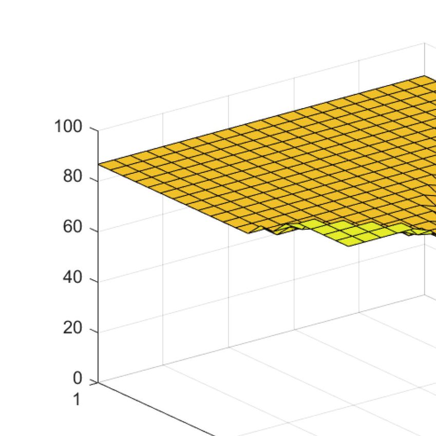
Sustainability 2020, 12, 6770                                                                       2 of 26

regarding locations and the capacity of facilities, quantity of products, distribution patterns, etc.,
to optimize the resource allocation in the entire network, on the basis of comprehensively considering
corporate social responsibility, sustainability or customer service level beyond the economic objectives,
as stated by many researchers. For instance, Pishvaee and Torabi [6] optimized the customer service
level by minimizing the delayed delivery time and formulating a bi-objective model. Khajavi [7]
investigated the integration of forward and reverse logistics networks with the minimum cost and
maximum response ability. Tuzkaya et al. [2] measured the customer service level by the defect rate of
products and maximized the weight of product flows from the initial recycling points to the centralized
recycling centers while minimizing the total cost. Ozkir and Basligil [5] studied the design of a
recycling network including three recycling levels, with the aim of maximizing transaction satisfaction,
customer satisfaction and total profit. Based on their research, Soleimani et al. [8] put forward two
indicators—carbon emission and time off work—to enhance the sustainability of the CLSC network.
Pourjavad et al. [9] minimized the total cost and lowered the environmental impact simultaneously.
Jiang et al. [3] advanced a CLSC network considering enterprise profit and service level simultaneously.
      On the other hand, with the purpose of tackling the uncertainty in the CLSC network (see Table 1),
stochastic programming and fuzzy programming have been extensively applied. In the former method,
the distributions of the parameters are usually obtained by the statistical analyses of historical data
(e.g., [10–12]). However, while lacking sufficient historical data, the distribution functions of some
uncertain parameters cannot be precisely estimated. Under this circumstance, people often evaluate
these parameters based on experience, thus, fuzzy set theory has emerged. Since it was initiated by
Zadeh [13] in 1965, it has been universally used in many fields, and the design of the uncertain CLSC
followed closely afterwards. For instance, based on the single-objective interaction method established
by Jimenez et al. [14] following fuzzy theory, Pishvaee and Torabi [6] advanced a multi-objective
fuzzy interactive method and applied it to the design of a multi-cycle CLSC network under fuzzy
environments. Then, a multi-product and multi-facility CLSC with capacity limitation was explored in
the work of Jindal and Sangwan [15] by building a fuzzy mixed integer linear programming (MILP)
model. ÖZceylan and Paksoy [16] formulated a multi-objective non-linear fuzzy programming model
and proposed an improved multi-objective fuzzy interaction method for CLSC planning. Recently,
a fuzzy multi-objective MILP model was extended to simulate the CLSC network by Pourjavad and
Mayorga [17], which was solved by their two-stage solution framework.
      The existing literature has also discussed the design of the CLSC with multiple recycling modes to
simulate the most realistic scene. In effect, large numbers of products are characterized by a modular
structured design as well as a long lifecycle [18]. Therefore, various recovery modes are required to deal
with returned goods with different service lives and quality levels. In the present work, we explore
the CLSC network design with the twin objectives of maximizing company profit and customer
satisfaction level under fuzzy environments. Refurbishment, repair, remanufacturing, recycling,
secondary market and disposal are the mainstream methods of recovery. Since refurbishment and
repair share the same resource flows, we treat them as one mode. The studies considering multiple
recovery options in the CLSC network design are listed in Table 1. Furthermore, the goals of CLSC
are multitudinous, from minimum cost, maximum profit, maximum customer satisfaction level to
corporate social responsibility or their combination, highlighting the different purposes of enterprises.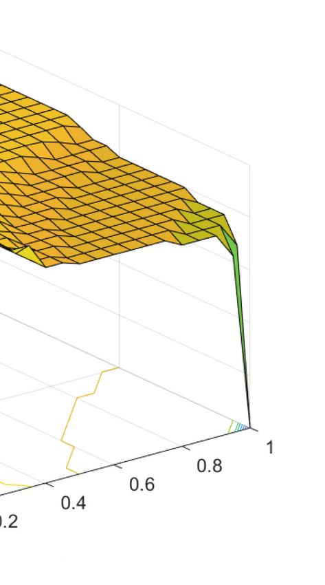
Sustainability 2020, 12, 6770                                                                                      3 of 26

            Table 1. CLSC network design problems with multiple recovery options under uncertainty

                                             Recovery Options                         Goals              Uncertainty
  Paper
                                    REP     REM      RCY     SM     DSP     MC     MP     MS     CSR     STO       FZY
                                             √                       √      √                                       √
  Tuzkaya et al. [2]                 √                                              √      √                        √
  Ozkir and Basligil [5]             √                √                      √             √                        √
  Pishvaee and Torabi [6]            √        √       √              √              √             √                 √
  Soleimani et al. [8]               √                √              √       √                    √                 √
  Pourjavad and Mayorga [9]                           √              √       √             √                        √
  Khajavi et al. [7]                                                         √                            √
  Tang et al. [10]                   √        √                              √                            √
  Uster and Hwang [11]                                √       √      √              √                     √
  Ahmadi and Amin [12]               √                √              √              √                              √
  Jindal and Sangwan [15]
                                     √                               √       √                                     √
  ÖZceylan and Paksoy [16]                    √       √              √       √                    √                √
  Pourjavad and Mayorga [17]                  √       √       √      √              √                     √
  Jerbia et al. [19]                 √                √              √       √                    √                √
  Darbari et al. [20]                √                √              √       √                                     √
  Javid et al. [21]                           √                      √       √                    √       √
  Zhen et al. [22]                   √        √       √       √      √              √      √                       √
  Our work
          Abbreviations: REP, REM, RCY, SM, DSP, MC, MP, MS, CSR, STO and FZY stand for repairing,
          remunufacturing, recycling, secondary market, disposal, minimum cost, maximum profit, maximum customer
          satisfaction level, corporate social responsibility, stochastic and fuzzy, respectively.

      The tabulated summary presented in Table 1 shows different study prospectives for CLSC network
design under the condition of uncertainty. Drawing upon Pishvaee and Torabi [6], we measure the
customer satisfaction level by the delayed delivery time. Our paper expands upon the listed articles by
presenting a CLSC network which integrates multiple recovery options, including remanufacturing,
recycling, repair, selling to secondary markets and disposal, making this the most comprehensive study
compared with other papers as shown in Table 1. Moreover, we incorporate the uncertainty of cost,
recovery ratio, delivery time, product price and quality in the model. To the best of our knowledge,
very few research works have considered all of these complex uncertain factors together in one model.
      In summarize, this paper differentiates itself from the existing related research and contributes
to the study of the CLSC network design from the following aspects: (1) considering the most
comprehensive recovery options simultaneously, as compared to the other works in Table 1;
(2) establishing a fuzzy bi-objective MILP model which maximizes both company profit and customer
satisfaction level for the CLSC network design under fuzzy environments; (3) presenting a two-stage
fuzzy interactive solution framework to solve the formulated fuzzy optimization model by integrating
the fuzzy expected value operator, fuzzy ranking method and fuzzy interactive solution method;
(4) comparing the performance of the fuzzy CLSC model with the deterministic one in [3] by several
numerical experiments to demonstrate the importance and necessity of designing the CLSC network
under fuzzy environments.
      The remainder of this paper is organized as follows. Section 2 presents the problem description
and mathematical formulation of the CLSC network design. Section 3 discusses how to process the
fuzzy parameters in the formulated fuzzy bi-objective MILP model. Following that, a two-stage fuzzy
interactive solution framework for solving the MILP model is constructed in Section 4. In Section 5,
some numerical experiments and comparisons are conducted to verify the performance of the proposed
model and solution framework. Finally, some pivotal conclusions are addressed in Section 6.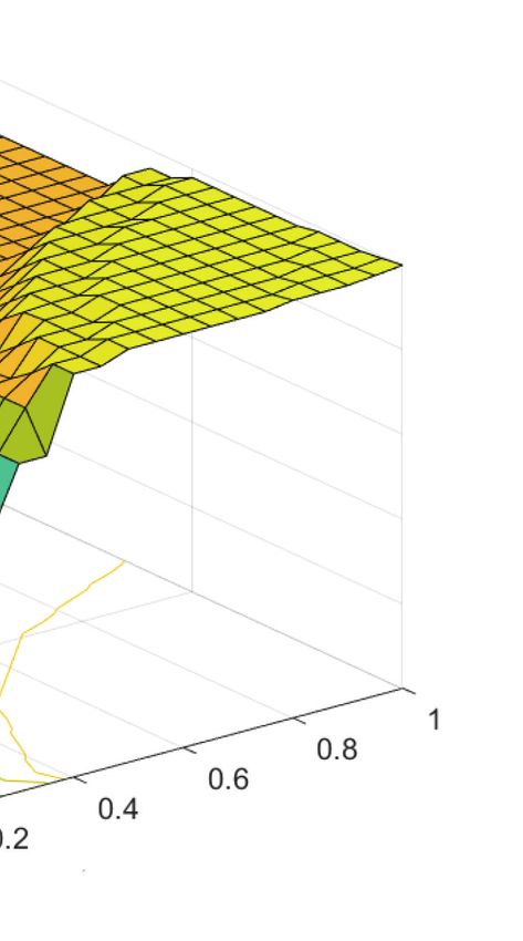
Sustainability 2020, 12, 6770                                                                                                   4 of 26

2. CLSC Network Design Under Fuzziness

2.1. Problem Description
       In Jiang et al. [3], the CLSC with multiple recovery options considering enterprise profit and
customer satisfaction under deterministic environments have already studied in a detailed manner,
and in this paper the problem is extended to a fuzzy one by inquiring into the impact of uncertainty
on the network design of the CLSC. Specifically, the discussed CLSC network consists of two
customer markets and various facilities serving these customers, such as plants, disposed material
processing centers and raw material recycling points, wherein the information of the customers
(i.e., demands, expected delivery time and degree of satisfaction), the cost coefficients (e.g., for start-up
cost, manufacturing cost or processing cost and unit transportation cost) and capacity of these facilities
and various recovery rates of recycled products are all fuzzy numbers. The structure of the CLSC and
its corresponding resource flow are depicted in Figure 1.
       As we can see, in the forward logistics, the plants process raw materials into new products and
transfer them to the primary customers through the distribution centers. In the reverse logistics, then,
the disassembly centers collect waste products from the primary customers, test or classify them and
determine their recovery modes within the following four options. The products with less damage are
directly repaired and then delivered to the secondary customers through the redistribution centers,
which are responsible for the delivery of the reprocessed products. The partially usable products are
disassembled at the disassembly centers and sent to the plants for remanufacturing and delivered to
the secondary customers through the redistribution centers afterwards. For the waste products that
cannot be repaired or used for remanufacturing, some useful raw materials are disassembled and
recycled at the raw material recycling points, and the worthless materials are sent to the processing
centers for disposal.

             Plants (I)                         Distribution centers (J)           Primary customers (K)

                                             For remanufacturing
                                  Remanufactured   ř                                    Returned
                             ř
                                                                           Disassembly centers (L)
             Second customers (N)         Redistribution centers (M)                                       Material recycling points

                                                                Repaired                       Recycled
                                                                   Ř                                Ś

                                                                                ś Disposed
                                                                           Processing centers (P)

                          Forward flow          Reverse flow

                                     Figure 1. The forward and reverse flows of the CLSC.

     The above-mentioned network provides a variety of recycling options, and thus can maximize
the recycling value of waste products. Meanwhile, the design separates the demand markets into
two parts, making the network more practical for the operation of many enterprises. Furthermore,
as a general network configuration with manufacturing-repairing-remanufacturing-recycling mode,
Sustainability 2020, 12, 6770                                                                                                  5 of 26

the proposed CLSC network can be diffusely used in the household electrical appliance manufacturing,
automobile industry, and other manufacturing industries.
      The purpose of the CLSC network design is to make decisions on the quantity and locations of the
facilities/the resource flow in the network, and the desirable configuration we aim to design is the one
that can bring economic benefits and increase operating efficiency, so as to help the enterprises improve
supply chain management, reduce energy consumption, waste emission and reinforce enterprise image.
In a network consisting of numerous entities, a series of activities involved will bring revenues to the
enterprises, but simultaneously increase operating costs. Consequently, the enterprises had should
more attention to the actual economic benefits brought by implementing the CLSC management.
Meanwhile, improving the efficiency of the network is conductive to reduce the delivery time and gain
customer satisfaction level, and ultimately enhance the economic value of the enterprises. Therefore,
this paper studies the design of a bi-objective CLSC network considering company profit and customer
satisfaction measured by the delayed delivery time.

2.2. Mathematical Formulation
          This section simplifies and abstracts the problem of the CLSC network design into a quantitative
fuzzy bi-objective optimization model. All of the parameters, decision variables, objective functions
and constraints involved are briefly introduced as follows (all notations used in the paper are collected
in Appendix A).
          Referring to the CLSC network structure displayed in Figure 1, the sets of the potential locations
of the plants, distribution centers, redistribution centers, disassembly centers and disposal centers,
and the fixed locations of the primary and secondary customers are denoted by I, J, M, L, P, K, and N,
respectively. Accordingly, the elements in these sets are respectively indexed by i, j, m, l, p, k, and n.
          Constructing and operating this network suffers three types of costs, i.e., the fixed facility
establishing cost, the variable processing or handling cost at these facilities and the transportation
cost between these facilities (and customers). The fixed start-up costs for plant i, distribution center j,
disassembly center l, redistribution center m and disposal center p are, respectively, represented by fei ,
fej , fel , fem and fep , with the maximum manufacturing or processing capacities of pei , pej , pel , pem , and pep ,
respectively. Correspondingly, the unit variable manufacturing or processing costs at these facilities
include the unit manufacturing cost mc         f i , unit remanufacturing cost vc           e i , unit handling costs hc     e j , hc
                                                                                                                                   e l,
hc
 e m , unit repairing cost rc     e l and unit disposing cost dc  e p . Furthermore, the unit transportation costs
between the facilities and customers are expressed as tc           e ij , tc
                                                                          e jk , tc
                                                                                 e li , tc
                                                                                        e lm , tc
                                                                                               e l p , tc
                                                                                                       e im and tc
                                                                                                                 e mn . Especially,
the unit collecting and transporting costs from primary customer k to disassembly center l are denoted
by cc  e kl . The maximum fraction of collecting waste products is ω,             e and the fractions of disposing and
repairing are θ1 and θ2 .
                    e        e
          Selling products and recycled raw materials are the main revenue sources of the CLSC. e                        s1 , e
                                                                                                                              s2 and
s3 denote the unit revenues of new products, remanufactured products and recycled raw materials,
e
respectively. The demands of primary customer k (purchases new products) and secondary customer
n (purchases remanufactured ones) are denoted by dek and den . In addition, a primary customer’s
satisfaction level is dependent on whether the products are delivered on time, which can be judged
by comparing the delivery time from distribution center j to customer k, dt                           e jk , with the customer’s
expected delivery time, eetk .
          To find out the optimal locations of the facilities in the network and the flow distribution among
them are the main tasks of the CLSC network design. Therefore, two kinds of decision variables
are included in the model. One is the continuous and positive variables used to represent the flows
between the facilities (and customers) in the network, and the other is the 0-1 variables used to indicate
whether a candidate site is selected for establishing the facility. These two kinds of decision variables
are expressed as Xij , X jk , Xkl , Xli , Xlm , Xl p , Xim , Xmn , Xl and Yi , Yj , Yl , Ym , Yp , respectively.
Sustainability 2020, 12, 6770 6 of 26
Considering the objectives of maximizing company profit (Z e1 ) and improving customer
satisfaction level by decreasing the delayed delivery time (Z
e2 ), the model of the fuzzy bi-objective
CLSC network design is expressed explicitly as follows,
max f − FC
e1 = TI
Z f − TC
f − MC
g − HC
g − CC
f − RMC
] − RC
f − DC
g
min Z e jk − eetk )+ X jk
e2 = ∑k∈K ∑ j∈ J (dt (1)
s.t. (A10)–(A26)
where TI, f FC,
f TC,f MC,g HC,g CC, f RMC,
] RC f and DC g are the total revenue, fixed establishment
cost, transportation cost, manufacturing cost, handling cost, collection cost of new products,
remanufacturing cost, repair cost and disposal cost of waste products, respectively. Detailed formulas
for the calculation of these terms as well as the constraint functions (A10)–(A26) are presented in
Appendix B.
Note that the problem of the fuzzy CLSC network design expounded in our paper is an extension
of the work presented in [3]. The settings of the two problems are identical except for the assumption
that the above parameters, whose notations have tilde symbols on their heads, are uncertain and
modeled as triangular fuzzy numbers here. Therefore, we only briefly introduce the fuzzy version of
the mathematical model and put the detailed formulas of the model in the appendix to keep this paper
self-contained. For more detailed descriptions and discussions on the CLSC network design problem
under deterministic environments, readers are recommended to [3].
It should be also noted that although the above model (1) is similar to the work of [3] in form, they
are quite different from each other in essence, since the model under fuzzy environments is of higher
complexity. Specifically, owing to the existence of the fuzzy parameters, the model cannot be directly
solved by the classic optimization techniques for deterministic programming models. Consequently,
in what follows, we discuss how to handle these fuzzy parameters and present a two-stage solution
framework to solve this fuzzy bi-objective programming model.
3. Processing Fuzzy Parameters in the CLSC Model
In model (1), both the objective functions and constraint functions contain fuzzy parameters.
Thus, the objectives cannot be directly optimized, and whether the constraints are satisfied cannot
be judged as well. Considering that, a general fuzzy programming model is formulated below as
model (2) for discussing how to manipulate these fuzzy parameters,
eT x
min Z e=C
s.t.
ei x ≥ Bei ,
A i = 1, 2, · · · , l (2)
ei x = Bei ,
A i = l + 1, · · · , m
x ≥ 0,
where x = ( x1 , x2 , · · · , x p ) is a p-dimensional vector representing the decision variables, A
ei and
T
C denote the fuzzy coefficient matrices of the constraints and the objective function, respectively,
e
and Bei is the vector representing the fuzzy bound of the constraints. Afterwards, by means of the
fuzzy expected value operator and fuzzy ranking method, the model can be transformed into its
deterministic counterpart, in which both the fuzzy objective functions and constraint functions in the
original model (1) are explicitly expressed.
Sustainability 2020, 12, 6770 7 of 26
3.1. Fuzzy Objective Functions
For converting the fuzzy objective functions into their crisp counterparts, it is natural to
approximate them by their expected values as illuminated by Jimenez et al. [23] and Liu [24]. To this
end, the definitions of the triangular fuzzy number (TFN) and the expected value of a TFN as well as
its linearity property should be elaborated in advance.
Definition 1. A TFN ξe = (ξ p , ξ m , ξ o ) is a fuzzy set on the real line, whose membership function can be
expressed as
x − ξp
p m
f ξ (x) = m p , if ξ ≤ x < ξ
−
ξ ξ
1, if x = ξ m
µξe( x ) =
ξo − x
gξ ( x ) = o , if ξ m < x ≤ ξ o
− m
ξ ξ
0, otherwise,
where f ξ ( x ) and gξ ( x ) are the left and right shape functions, and ξ p , ξ m , and ξ o are the lower bound, median
value, and upper bound, respectively, of the TFN, as shown in Figure 2.
Definition 2 (Jimenez et al. [23]). The expected interval (EI) and expected value (EV) of a TFN ξe =
(ξ p , ξ m , ξ o ) are, respectively,
1 Z 1
Z
1
f e−1 ( x )dx, g− 1
= [ξ p + ξ m , ξ m + ξ o ] ,
ξe ξe
EI [ξe] = [ E1 , E2 ] = ( x ) dx
0 ξ 0 ξe 2
ξe ξe
E1 + E2 ξ p + 2ξ m + ξ o
EV [ξe] = = .
2 4
1
0 x
Figure 2. Membership function of ξe = (ξ p , ξ m , ξ o ).
Theorem 1 (Jimenez et al. [23]). Let ξe and ζe be two TFNs. For any real numbers a and b, we have
EV [ aξe + bζe] = aEV [ξe] + bEV [ζe].
According to the above theorem, we convert the expected value of the fuzzy objective function Z
e1
in model (1) into the following form,
EV [ Z f ] − EV [ FC
e1 ] = EV [ TI f ] − EV [ TC
f ] − EV [ MC
g ] − EV [ HC
g ] − EV [CC
f ] − EV [ RMC
] ] − EV [ RC
f ] − EV [ DC
g ], (3)Sustainability 2020, 12, 6770 8 of 26
where EV [ TI
f ] can be further calculated as
p p p
! ! !
s1 + 2s1m + s1o s2 + 2s2m + s2o s3 + 2s3m + s3o
EV [ TI
f] = ∑∑ 4
X jk + ∑ ∑ 4
Xmn + ∑ 4
Xl , (4)
j∈ J k∈K m∈ M n∈ N l∈L
p p p
where s1 /s2 /s3 , s1m /s2m /s3m , s1o /s2o /s3o represent the lower bound, mean value and upper bound of
the unit revenue of new products/remanufactured products/recycled raw materials, respectively.
Likewise, EV [ FC
f ], EV [ TC f ], EV [ MC g ], EV [ HC
g ], EV [CC
f ], EV [ RMC
] ], EV [ RC
f ] and EV [ DC
g ] can be
calculated according to the definition of EV.
However, the second objective function Z
e2 in model (1) cannot be similarly calculated as presented
above by applying the linearity of the EV operator (Theorem 1) owing to the existence of the operator
(·)+ . In some previous studies, the operator was simply approximated, such that
e − eet)+ ] = ( EV [dt
EV [(dt e ] − EV [eet])+ , (5)
where dt
e and eet are TFNs (see, e.g., [6]). Clearly, this treatment would lead to serious deviation from the
real exact value in some cases. Therefore, in this paper, based on the concepts of EI and EV proposed
by Jimenez et al. [23], we exactly calculate the value of EV [(dt e − eet)+ ] as follows,
g )+
( Tdt g )+
( Tdt
+ E2 1 Z 1
g )+ ] = E1
Z
1
EV [( Tdt = f −g1
( x )dx + g−g 1
( x )dx , (6)
2 2 0 ( Tdt)+ 0 ( Tdt)+
g = dt
where Tdt g )+ may not be.
e − eet is still a TFN, whereas ( Tdt
Take dt = (3.2, 6.2, 8.6) and eet = (2.3, 4.3, 5.7) for example. Undoubtedly, Tdt
e g = dt e − eet =
(−2.5, 1.9, 6.3) is a TFN. However, ( Tdt +
g ) is not, since it is a nonnegative fuzzy number, as displayed
in Figure 3a. In light of Equation (6), we have EV [( Tdt g )+ ] = 3969 ≈ 2.3, which is different from
1760
+
( EV [dt] − EV [eet]) = 6.05 − 4.15 = 1.9.
e
1 1
-2.5 0 1.9 6.3 x -4.8 -0.6 0 4.0 x
(a) (b)
g )+ .
Figure 3. Membership function of ( Tdt
e = (2.6, 5.0, 7.0) and eet = (3.0, 5.6, 7.4). Then Tdt
Again, let dt g = dt e − eet = (−4.8, −0.6, 4.0),
+
and the membership function of ( Tdt) is as shown in Figure 3b. It can be decuced by Equation (6)
g
e − eet)+ ] = 20 ≈ 0.9, whereas ( EV [dt
that EV [(dt e ] − EV [eet])+ = (4.9 − 5.4)+ is 0. These two examples
23
illustrate the superiority of the proposed method over the approximation methods such as in [6].
3.2. Fuzzy Constraint Functions
Analogously, with the purpose of determining whether a constraint with fuzzy parameters is
valid, the method proposed by Jimenez et al. [23] for comparing two fuzzy numbers is adopted in this
paper as follows.Sustainability 2020, 12, 6770 9 of 26
Definition 3 (Jimenez et al. [23]). For TFNs ξe and ηe, the degree of ξe > ηe is defined as
ξe ηe
0, if E2 − E1 < 0
ξe ηe
E2 − E1
ξe ηe ξe ηe
µ M (ξ,
e ηe) = , if 0 ∈ [ E1 − E2 , E2 − E1 ]
ξe ξe ηe ηe
E2 − E1 + E2 − E1
ξe ηe
1, if E1 − E2 > 0,
ξe ξe ηe ηe e ηe) ≥ α, we mark it as ξe ≥α ηe.
where [ E1 , E2 ] and [ E1 , E2 ] are EI of ξe and ηe, respectively. Especially, if µ M (ξ,
ei x ≥α B
After applying the above definition into model (2), the constraints A ei , i = 1, 2, · · · , l, are
equivalent to the following group of equations,
ex
A B
E2 i − E1 i
e
ex ex
≥ α, i = 1, 2, · · · , l,
A A B B
E2 i − E1 i + E2 i − E1 i
e e
namely,
[(1 − α) E2Ai + αE1Ai ] x ≥ αE2Bi + (1 − α) E1Bi , i = 1, 2, · · · , l,
e e e e
(7)
ei x ≥ B
where α is the confidence level used to adjust the degree of the constraints A ei being valid.
Similarly, the degree of equality of two fuzzy numbers was defined by Parra et al. [25] below.
Definition 4 (Parra et al. [25]). For any two TFNs ξe and ηe, we have ξe ≈α ηe, if ξe ≤ α ηe and ηe ≤ α ξ,
e i.e.,
2 2
α e ηe) ≤ 1 − α .
≤ µ M (ξ,
2 2
There are three kinds of constraints in the fuzzy programming model (2), including the fuzzy
inequality, fuzzy equation and crisp constraints. According to Definition 3, the fuzzy inequality
constraints can be transformed into the corresponding deterministic inequality ones formulated as
Equation (7). Furthermore, the fuzzy equality constraints can be converted into
ex
A B
E2 i − E1 i
e
α α
≤ e ≤ 1− , i = l + 1, · · · , m,
2 Ai x ei x
A B
ei
E2 − E1 + E2 − E1
B
ei 2
and further expressed as
h α Aei α Aei i α Be α Bei
1− E2 + E1 x ≥ E2 i + 1 − E1 , i = l + 1, · · · , m, (8)
2 2 2 2
α fA
α f A
α Bei α Bei
E2 i + 1 − E1 i x ≤ 1 − E2 + E1 , i = l + 1, · · · , m (9)
2 2 2 2
according to Definition 4.
3.3. Transformation
Referring to the methods presented before, the general form of a fuzzy programming model (2)
can be transformed into the following deterministic counterpart,
eT ] x
min EV [C
s.t. (7)–(9) (10)
x ≥ 0.
Sustainability 2020, 12, 6770 10 of 26
By converting model (2) into model (10), the fuzzy inequality constraints are transformed into
a group of crisp inequalities, and the fuzzy equality constraints are converted into two groups of
crisp inequality constraints, respectively, with the confidence level of α, whereas the crisp ones
are maintained.
Similarly, the fuzzy constraints in the fuzzy CLSC model (1), i.e., (A10), (A11), (A13),
(A15)–(A17), (A20)–(A24), are, respectively, transformed into the crisp ones as follows,
α θ p + θm α θo + θm
1−
2 2
− 1−
2 2 ∑ Xkl ≤ ∑ Xli + Xl , ∀l ∈ L, (11)
k∈K i∈ I
α θ p + θm α θo + θm
1− 1−
2 2
−
2 2 ∑ Xkl ≥ ∑ Xli + Xl∈L , ∀l ∈ L, (12)
k∈K i∈ I
p
!
dn + dm don + dm
∑ Xmn ≤ α
2
n
+ (1 − α )
2
n
, ∀n ∈ N, (13)
m∈ M
p
ω + ωm
o
ω + ωm
∑ klX ≤ α
2
+ ( 1 − α )
2 ∑ Xjk , ∀k ∈ K, (14)
l∈L j∈ J
p
" #
α θo + θm α θ1 + θ1m
2
1
2
1
+ 1−
2 2 ∑ Xkl ≤ ∑ Xl p , ∀l ∈ L, (15)
k∈K m∈ M
p
" #
α θ1o + θ1m α θ1 + θ1m
1−
2 2
+
2 2 ∑ Xkl ≥ ∑ Xl p , ∀l ∈ L, (16)
k∈K m∈ M
p
" #
α θo + θm α θ2 + θ2m
2
2
2
2
+ 1−
2 2 ∑ Xkl ≤ ∑ Xlm , ∀l ∈ L, (17)
k∈K m∈ M
p
" #
α θ2o + θ2m α θ2 + θ2m
1−
2 2
+
2 2 ∑ Xkl ≥ ∑ Xlm , ∀l ∈ L, (18)
k∈K m∈ M
p
α do + dm α dk + dm
∑ Xjk ≥ 2
k
2
k
+ 1−
2 2
k
, ∀k ∈ K, (19)
j∈ J
α dok + dm α d p + dm
∑ jk X ≤ 1 −
2 2
k
+
2
k
2
k
, ∀k ∈ K, (20)
j∈ J
p
" ! #
pi + pim pio + pim
∑ Xij + ∑ Xim ≤ α
2
+ (1 − α )
2
Yi , ∀i ∈ I, (21)
j∈ J m∈ M
p
p j + pm poj + pm
" ! !#
j j
∑ Xjk ≤ α
2
+ (1 − α )
2
Yj , ∀ j ∈ J, (22)
k∈K
p
" ! #
pl + pm pol + pm
∑ Xkl ≤ α
2
l
+ (1 − α )
2
l
Yl , ∀l ∈ L, (23)
k∈K
p
" ! #
pm + pm pom + pm
∑ Xmn ≤ α
2
m
+ (1 − α )
2
m
Ym , ∀m ∈ M, (24)
n∈ NSustainability 2020, 12, 6770 11 of 26
p
p p + pm pop + pm
" ! #
p p
∑ Xl p ≤ α
2
+ (1 − α )
2
Yp , ∀ p ∈ P. (25)
l∈L
Consequently, a deterministic counterpart of the fuzzy CLSC model (1) is deduced as follows,
max Z1 = EV [ Z f ] − EV [ FC
e1 ] = EV [ TI f ] − EV [ TCf ] − EV [ MCg ] − EV [ HC
g]
− EV [CC
f ] − EV [ RMC
] ] − EV [ RC f ] − EV [ DC
g]
min Z2 = EV [ Z e jk − eetk )+ ] X jk
e2 ] = ∑k∈K ∑ j∈ J EV [(dt
s.t.
∑i∈ I Xij = ∑k∈K X jk , ∀ j ∈ J
∑k∈K Xkl = ∑i∈ I Xli + ∑m∈ M Xlm + ∑ p∈ P Xl p + Xl , ∀l ∈ L (26)
∑l ∈ L Xli = ∑m∈ M Xim ,
∀i ∈ I
∑i∈ I Xim + ∑l ∈ L Xlm = ∑n∈ N Xmn , ∀m ∈ M
(11)–(25)
Yi , Yj , Yl , Ym , Yp ∈ {0, 1}, ∀i, j, l, m, p
Xij , X jk , Xkl , Xli , Xlm , Xl p , Xim , Xmn , Xl ≥ 0, ∀i, j, k, l, m, n, p.
where the EVs of (A2)–(A9) are calculated as Equation (4), and EV [(dt e jk − eetk )+ ] is calculated by
Equation (6).
So far, the fuzzy bi-objective model (1) for the problem of designing a fuzzy CLSC network has
been converted into a crisp bi-objective mixed 0-1 integer linear programming (CB-MILP) model (26).
In order to achieve a compromise between the two objectives within the model, a solution framework
on the basis of the fuzzy interactive approach is proposed in the following section.
4. Solution Framework for the Fuzzy CLSC Model
4.1. Interactive Approach to Multi-Objective Programming
Multi-objective programming is a model that optimizes multiple objectives simultaneously while
the constraints are all satisfied, whose general form is
(
min f ( x) = ( f 1 ( x), f 2 ( x), · · · , f m ( x))
(27)
s.t. x ∈ S,
where x = ( x1 , x2 , · · · , x p ) is a p-dimensional decision vector, f 1 ( x), · · · , f m ( x) are m objective
functions, and the feasible set is denoted by S.
In order to solve this kind of multi-objective problems, Zimmermann [26] proposed a fuzzy
interaction method, in which the implementation degree of each exact objective is provided according
to the preferences. The method can help to transform a multi-objective programming into a
single-objective Min-Max model, thereby balancing multiple goals. While being applied, some
expansions have been made by Werners [27], Torabi and Hassini [28] (called the TH method) and Selim
and Ozkarahan [29] (called the SO method). idea of the Min-Max model is to construct the membership
function of the target value so as to quantify the fuzzy target of decision-makers. Subsequently, based
on the membership function of each objective, a synthesis evaluation function of the single objective
is constructed to optimize the interaction among different objectives, and then the optimal solution
is obtained. Therefore, the key of applying this method lies in the construction of the membership
function and synthesis evaluation function.Sustainability 2020, 12, 6770 12 of 26
To do so, we first determine the membership function of objective i (1 ≤ i ≤ m), say µi ( x ). As a
preliminary step, the positive ideal solution (PIS) and negative ideal solution (NIS) of each objective
are calculated. In model (27), there are m objectives of minimization, and thus the minimum value
of each objective function is the corresponding PIS, recorded as f iPIS = min f i ( x), x ∈ S. After that,
fix the objective function and plug the other x values into it, then the maximum objective function
value can be deduced as f iN IS . For instance, letting m = 3, we have the PIS of each objective and the
corresponding decision vector x, i.e., ( f 1PIS , x1 ), ( f 2PIS , x2 ), ( f 3PIS , x3 ), respectively. Then, the NIS of each
objective is,
f 1N IS = f 1 ( x2 ) ∨ f 1 ( x3 ), f 2N IS = f 2 ( x1 ) ∨ f 2 ( x3 ), f 3N IS = f 3 ( x1 ) ∨ f 3 ( x2 ). (28)
Based on the concepts of PIS and NIS, the membership function µi ( x ) is constructed by combining
the subjective preferences of decision-makers, among which the most commonly used linear form is
shown below,
if x > f iN IS
0,
f N IS − x
i
µi ( x ) =
N IS − f PIS
, if f iPIS ≤ x ≤ f iN IS (29)
f i i
if x < f iPIS .
1,
Second, combining with the membership function in Equation (29), we employ the synthesis
evaluation function λ(x) to convert the bi-objective model (26) into a single one by means of the TH
method [28], which adds the compensation factor γ on the basis of Min-Max method as follows,
max λ(x) = γλ0 + (1 − γ) ∑ g w g µ g ( Zg (x))
s.t.
(30)
λ0 ≤ µ g ( Zg (x)), g = 1, 2
x ∈ F,
where x is the decision vector consisting of continuous and 0–1 variables, Zg (x) = EV [ Z eg (x)], g = 1, 2,
and F represent the objective functions and feasible set of model (26), respectively, and w g represents
the predetermined importance weights of different objectives.
It should be pointed out that the decision variable λ0 = ming {µ g ( Zg (x))} expresses the minimum
implementation level of the objective function, and γ ∈ [0, 1] is the compensation factor of the
minimum implementation level. Through the TH evaluation function, we find that a trade-off between
the weighted and the minimum operators can be achieved, hence the decision-makers can adjust the
parameters w g and γ to obtain equilibrium and non-equilibrium solutions between the two objectives
according to their preferences.
4.2. Two-Stage Fuzzy Interaction Solution Procedure
As elaborated in Sections 3 and 4.1, the solution framework for solving the problem of the fuzzy
CLSC network design can be integrated into a two-stage fuzzy interaction solution procedure. In the
first stage, transform the original fuzzy bi-objective CLSC model (1) into a crisp bi-objective MILP
model (26) with the feasibility level, α, based on the fuzzy expected value theory and fuzzy ranking
method introduced by Jimenezi et al. [23], as performed in Section 3. Following that, by means of the
fuzzy interaction method proposed by Zimmermann [26] and improved by Torabi and Hassini [28],
the crisp bi-objective MILP model is turned into a deterministic single-objective model (30) in the
second stage, as presented in Section 4.1. Since the fuzzy interaction method calculates the realization
level of each objective function directly, decision-makers can obtain equilibrium solutions between
multiple objectives and non-equilibrium solutions with their subjective preferences, and provide
a variety of valuable decision-making schemes by adjusting the related parameters including theSustainability 2020, 12, 6770 13 of 26
feasibility level α, the compensation factor γ and the weight coefficient w g . In a word, the specific steps
of the two-stage fuzzy interaction solution method can be depicted in Figure 4 and summarized in
the following:
PIS and NIS for
Fuzzy objective Crisp form of objectives (28)
Definition 2
functions objectives
A(1) — A(9) Theorem 1 (3) (4) (6)
TH method Realization level of
objectives (29)
Fuzzy
Definition 3 Crip inequalities
Constraints Synthesis evaluation
Definition 4 (11) — (25)
(A10) — (A26) function (30)
Fuzzy bi-objective Crisp bi-objective Deterministic single-
CLSC model (1) MILP (26) objective MILP (30)
Stage 1 Stage 2
Figure 4. Process of two-stage fuzzy interaction solution.
Step 1: Transform the objective functions with fuzzy parameters, Z e1 and Z e2 in the original CLSC
model (1), into the crisp form, Z1 and Z2 in model (26), by means of the fuzzy expected value
theory elaborated in Definition 2 and Theorem 1.
Step 2: Determine the minimum feasibility level α of model (1), and convert the fuzzy constraints
(A10)–(A26) into their explicit inequality counterparts (11)–(25) according to Definition 4, so as
to construct the crisp bi-objective MILP model (26).
Step 3: Calculate the PIS Z1α-PIS and Z2α-PIS for each objective at the feasibility level α and the
corresponding decision schemes x1 α-PIS and x2 α-PIS , and then figure out Z1α-N IS = Z1 (x2 α-PIS ),
Z2α-N IS = Z2 (x1 α-PIS ).
Step 4: Based on the PIS and NIS, compute the realization levels of the objectives in model (26), µ g ( x ),
which are definitely constructed as follows,
if x < Z1α− N IS
0,
x − Z1α-N IS
µ1 ( x ) = , if Z1α-N IS ≤ x ≤ Z1α-PIS
Z1α-PIS − Z1α-N IS
1, if x > Z1α-PIS ,
0, if x > Z2α-N IS
Z2α-N IS − x
µ2 ( x ) = , if Z2α-PIS ≤ x ≤ Z2α-N IS
Z2α-N IS − Z2α-PIS
1, if x < Z2α-PIS .
Step 5: Establish the synthesis evaluation function λ(x) via the multi-objective interactive TH method
to convert the CB-MILP model (26) into a deterministic single-objective MILP model (30),
and then determine the compensation factor γ and the weight coefficients w g of the evaluation
function to solve it.
Step 6: Adjust the parameters α, γ (if necessary, the weight coefficients w g can be changed), and repeat
Steps 2–6 until the solution is satisfactory from the perspective of the decision-maker.Sustainability 2020, 12, 6770 14 of 26
5. Numerical Analysis
To confirm the validity of the transformed CB-MILP model and the proposed solution framework,
some numerical experiments are conducted in this section. Afterwards, some comparisons with the
deterministic problem solved by Jiang et al. [3] is presented. All the experiments in this paper were
run in the computer environment of Intel(R) Core(TM) i5-8265@1.60ghz, and the solutions are derived
from CPLEX 12.8.0 called by Matlab 2018 R(b).
5.1. Experimental data
The experiments consider a CLSC network with 43 sites, including 4 factory alternative points,
8 distribution center alternative points, 12 primary customer points, 6 disassembly center alternative
points, 4 alternatives for redistribution centers, 6 secondary customer points and 3 alternatives for
processing centers. More details of the sites are accessible in [3]. The fuzzy parameters in the problem
are all assumed as TFNs, the lower bound, median value and upper bound of which are generated
following the uniform distribution. The specified process is as follows. First, randomly generate a
median value of ξ m for each parameter. Second, in order to avoid loss of generality, generate two
random numbers (τ1 ,τ2 ) following the uniform distribution between 0.2 and 0.5, respectively, as the
left and right spreads. Third, calculate the lower and upper bounds of TFN ξ, e ξ p and ξ o , as
ξ p = (1 − τ1 )ξ m , ξ o = (1 + τ2 )ξ m .
To facilitate the comparisons between our work with the deterministic problem, the medians of
the fuzzy numbers are set as the corresponding deterministic values in [3]. Furthermore, the left and
right spreads, (τ1 , τ2 ), are randomly generated as shown in Table 2.
Table 2. Left and right spreads of fuzzy parameters.
Parameter (τ1 , τ2 ) Parameter (τ1 , τ2 ) Parameter (τ1 , τ2 )
fei (0.31, 0.41) tc
e li (0.43, 0.41) cc
e kl (0.39, 0.49)
fej (0.31, 0.48) tc
e lm (0.37, 0.25) dek (0.28, 0.34)
fel (0.22, 0.41) tc
e lp (0.29, 0.24) den (0.43, 0.37)
fem (0.41, 0.39) tc
e im (0.44, 0.29) ω
e (0.29, 0.43)
fep (0.33, 0.30) tc
e mn (0.29, 0.25) θe1 (0.23, 0.42)
pei (0.28, 0.40) mc
fi (0.21, 0.22) θe2 (0.37, 0.29)
pej (0.43, 0.28) vc
ei (0.43, 0.21) dt
e jk (0.49, 0.40)
pel (0.25, 0.32) rc
el (0.29, 0.26) eetk (0.46, 0.33)
pem (0.24, 0.43) dc
ep (0.33, 0.21) s1
e (0.20, 0.40)
pep (0.48, 0.27) hc
ej (0.23, 0.20) s2
e (0.31, 0.33)
tc
e ij (0.26, 0.48) hc
el (0.38, 0.33) s3
e (0.29, 0.34)
tc
e jk (0.37, 0.39) hcm
e (0.34, 0.37)
5.2. Two-Stage Fuzzy Interaction Analysis
For solving the above problem, we plug the parameters into the fuzzy bi-objective programming
model (1), carry out the crisp equivalence transformation, and obtain the CB-MILP model (26) for the
experiments. Afterwards, by setting different feasibility levels α, the PIS of the profit and the NIS of the
delayed delivery time representing the optimal solution results when only one of the two objectives
is considered are figured out, as shown in Figure 5. It can be observed that, with the increase of α,
the optimal value of the profit marked by the dotted black line decreases, and the optimal value of the
delayed delivery time represented by the solid blue line increases. Since the objective functions as well
as the constraints of model (1) are all linear combinations of the triangular fuzzy parameters, the two
lines are changing in a linear fashion.Sustainability 2020, 12, 6770 15 of 26
Then, substitute the optimal decision scheme of one goal into the other according to Equation (28),
we obtain the worst values of the two goals, i.e., the NIS of the profit and the PIS of the delayed
delivery time, as presented in Figure 5. Obviously, with the increase of α, the worst cases show a
strict monotone tendency and the differences between the PIS and NIS of the objective functions both
shrink. As mentioned in Section 4.1, the PIS and NIS prescribe a limit to the range of one objective
while another objective is optimized, thus Figure 5 indicates that the range of the two objectives
narrows with the increase of α. This trend is consistent with common sense, since the feasibility level,
α, is a parameter representing the degree of constraint relaxation, i.e., a higher feasibility level is
equivalent to a greater degree of constraints satisfaction and a smaller feasible region of the solution.
The experimental results can provide decision-makers with the range of the two objective functions at
different feasibility levels and help to avoid the risks caused by uncertain factors.
106 104
5 2.5
4.5
Delayed delivery time
2
4
Profit
PIS of profit
NIS of profit
NIS of time
3.5 PIS of time
1.5
3
2.5 1
0 0.2 0.4 0.6 0.8 1
Feasibility level (α)
Figure 5. PIS and NIS of the fuzzy CLSC model at different feasibility levels.
Based on the above PIS and NIS of the two objectives at different feasibility levels with the weight
coefficients of w1 = w2 = 0.5, namely, maximizing the profit is as important as minimizing the delayed
delivery time, and the compensation factor of γ = 0.5, the realization levels of the two objectives, µ1
and µ2 , by using the TH fuzzy interaction method are obtained as shown in Table 3. In general, with the
increase of α, the realization levels of the two objectives are relatively high and experience strictly
monotone increasing trends. Typically, when α = 0, the most relaxed constraints result in the largest
feasible region, and the solution which can immunize against the largest parameter perturbation is
achieved, with the minimum realization levels of the two objectives, 80.29%. By contrast, when it
comes to α = 1, the tightest constraints lead to the most reliable results with the realization levels of
95.32% and 98.33%. Furthermore, the average realization levels are, respectively, 87.47% and 87.74%,
indicating that the TH method is competent to obtain stable and precise solutions.
Table 3. Realization levels of the two objectives with different feasibility levels (γ = 0.5).
α 0 0.1 0.2 0.3 0.4 0.5 0.6 0.7 0.8 0.9 1 Average
µ1 (%) 80.29 81.64 82.98 84.30 85.06 86.81 88.46 89.93 92.20 95.18 95.32 87.47
µ2 (%) 80.29 81.64 82.98 84.30 85.06 86.81 88.46 89.93 92.20 95.18 98.33 87.74
On the other hand, we can see from Table 3 that there is little difference between the realization
levels, the reason is that the compensation factor is set to be 0.5, and accordingly the objective function
of model (30), λ = 0.75 min{µ1 , µ2 } + 0.25 max{µ1 , µ2 }, endows a greater weight to the goal with lower
realization level, which means the model pays more attention to the short board and is aimed to obtain
a compromise and equilibrium solution between the two objectives. For more information, we set theSustainability 2020, 12, 6770 16 of 26
compensation factor as γ = 0, i.e., λ = 0.5µ1 + 0.5µ2 , and record the realization levels as well as the
gap between them, µ1 − µ2 , at different feasibility levels in Table 4. The results explicitly show that the
gap tends to decrease with the increase of α and the realization levels of maximizing enterprise profit
is constantly higher than that of minimizing customers’ delayed delivery time except for the case of
α = 1, demonstrating that the most balanced solution can be obtained when α is between 0.9 and 1.
Table 4. Realization levels of the two objectives with different feasibility levels (γ = 0).
α 0 0.1 0.2 0.3 0.4 0.5 0.6 0.7 0.8 0.9 1 Average
µ1 (%) 98.26 98.22 98.16 98.06 97.94 97.76 97.57 97.30 96.95 96.49 94.40 97.28
µ2 (%) 67.59 71.30 72.48 75.01 77.36 79.93 82.75 85.90 89.67 94.54 99.98 81.50
Gap (%) 30.67 26.92 25.68 23.05 20.58 17.83 14.82 11.40 7.28 1.95 −5.58 15.78
Therefore, to further explore the sensitivity of the TH method to γ, we fix the feasibility level at 0.9
after comparing the solutions of different α and figure out the realization levels of the two objectives as
well as the gap between them, µ1 − µ2 , as illustrated in Table 5. It shows that the TH method tends
to seek equilibrium solutions, for the gap narrows down with the increase of γ. Especially, when
γ ≥ 0.4, µ1 is equal to µ2 and is constantly unchanged. That is, as γ gradually approaches 1, the results
pays more attention to optimize the objective with lower realization level, so that a more equilibrium
state can be reached. Additionally, we find that µ1 and µ2 evince similar trend of monotonic increase,
which is consistent with the conclusion of [28], verifying the remarkable monotonicity of multiple
realization levels with the increase of γ while introducing the TH method. Besides, it should be pointed
out that, at a fixed feasibility level, when the compensation factor γ is small, the TH method can obtain
non-equilibrium solutions between multiple objectives, as the realization levels are relatively high.
Table 5. Realization levels and gap with different γ.
γ 0 0.1 0.2 0.3 0.4 0.5 0.6 0.7 0.8 0.9 1
µ1 (%) 96.49 96.49 96.48 96.48 95.18 95.18 95.18 95.18 95.18 95.18 95.18
µ2 (%) 94.54 94.54 94.54 94.54 95.18 95.18 95.18 95.18 95.18 95.18 95.18
Gap (%) 1.95 1.95 1.94 1.94 0.00 0.00 0.00 0.00 0.00 0.00 0.00
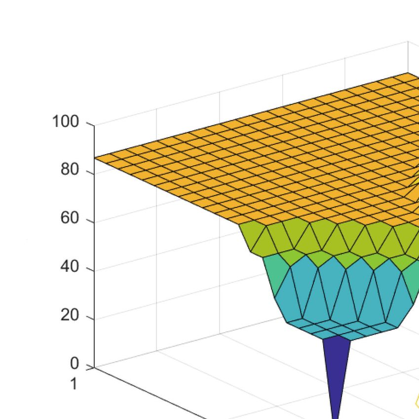
Ultimately, in order to investigate the joint effect of the weight coefficients and the compensation
factor (w1 , w2 and γ) on the realization levels of the two objectives, we fix α at 0.5 and accordingly
depict the results in Figure 6. It can be seen from Figure 6a that the weight coefficients of the two
objectives have no effect on the realization level of maximizing the enterprise’s profit when γ > 0.6
(with µ1 remaining steady at 90%), yet have significant influence when it comes to γ ≤ 0.6. Specifically,
when w1 ≥ 0.4 (w2 ≤ 0.6), µ1 maintains a high level of more than 90%; and when w1 < 0.4 (w2 > 0.6)
and γ ≤ 0.6, it decreases rapidly and reaches the bottom of 0 with w1 = 0 and γ = 0. In Figure 6b,
the similar conclusion can be drawn as Figure 6a since the tendency of µ2 in Figure 6b is close to that
of µ1 in Figure 6a if the x-axis, w1 , is replaced by w2 . Hence, to get more equilibrium solutions, it is
supposed to set a relatively concentrated value of w1 and w2 and a relatively high value of γ.Sustainability 2020, 12, 6770 17 of 26
5HDOL]DWLRQOHYHORIPLQLPL]LQJ
5HDOL]DWLRQOHYHORI GHOD\HGGHOLYHU\WLPH Ǎ2
PD[LPL]LQJSURILW Ǎ
&R &R
PS PS
HQVDW ǚ HQV ǚ
LW DWLR URILW
LRQ SURI LQJS
IDF L]LQJ QI
DFW [LPL]
WRU D[LP RU D
DŽ RIP RIP
: HLJKW DŽ
: HLJKW
D E
Figure 6. The realization levels of the two objectives with different weight coefficients and compensation
factors.
To sum up, the above analyses show that while designing the CLSC network in fuzzy
environments, the decision-makers can obtain satisfactory solutions by modifying the parameters,
i.e., the feasibility level, the compensation factor, and the weight coefficients, according to their
preferences, and the fuzzy settings provide more flexible and diversified options for decision-making.
In the next section, we will elaborate this advantage in detail by some comparisons with the
deterministic problem presented by [3].
5.3. Comparisons with the Deterministic Problem
By fixing the parameters at γ = w1 = w2 = 0.5 and solving the proposed fuzzy model and the
deterministic one in [3], the comparative results on the optimal solutions at different feasibility levels
are depicted in Table 6 and Figure 7.
Table 6. Optimal solutions of the fuzzy and the deterministic model at different feasibility levels.
α 0 0.1 0.2 0.3 0.4 0.5 0.6 0.7 0.8 0.9 1
Profit 4,518,735 4,477,079 4,444,595 4,410,003 4,363,774 4,316,022 4,274,709 4,226,976 4,182,241 4,136,117 4,071,544
Fuzzy
Time 14,336.6 14,291.9 14,285.6 14,270.3 14,301.8 14,233.5 14,194.8 14,189.8 14,144.0 14,103.0 14,092.1
Determ Profit 3,878,633 3,878,633 3,878,633 3,878,633 3,878,633 3,878,633 3,878,633 3,878,633 3,878,633 3,878,633 3,878,633
inistic Time 4701.0 4701.0 4701.0 4701.0 4701.0 4701.0 4701.0 4701.0 4701.0 4701.0 4701.0
'HOD\HGGHOLYHU\WLPH
3URILW
3URILW (deterministic)
3URILW(fuzzy)
7LPH (dHWHUPLQistic)
7LPH (fX]]y)
)HDVLELOLW\OHYHO ǂ
Figure 7. Comparisons of the objective values under fuzzy and deterministic environments with the
TH method at different feasibility levels.Sustainability 2020, 12, 6770 18 of 26
As we can see from the four curves representing the optimal solutions of the objective functions
obtained by using the TH method under deterministic and fuzzy environments, both the profit
and the delayed delivery time in the deterministic problem are less than that in the fuzzy one.
Furthermore, it also can be observed that the values of the two objectives under fuzzy environments
decrease with the feasibility level α increases, whereas the results under deterministic environment are
constantly unchanged.
Explicitly, the delayed delivery time in fuzzy cases is much longer. At the root, under deterministic
environments, Jiang et al. [3] calculated the delayed delivery time by adding up the non-negative
differences between the actual and the expected delivery time, which is equivalent to the treatment
of Equation (5) corresponding to the fuzzy cases. However, in our fuzzy settings, the difference
between the fuzzy expected delivery time and the fuzzy actual delayed delivery time are calculated by
Equation (6), since we have proved in Section 3 with concrete data that the difference between fuzzy
numbers cannot be directly calculated by their EVs and Equation (5) may result in a huge deviation.
Thus, a big gap between the delayed delivery time under different environments arises, as shown in
Figure 7.
On the other hand, minimizing the delayed delivery time and total profit are two conflicting
objectives, that is, a shorter delayed delivery time brings a higher service level and higher cost/lower
profit simultaneously. Therefore, in Figure 7, the profit under fuzzy environments is also larger than
the deterministic case. Specifically, the maximum disparity of the two lines, representing the profits
under different environments (4,518,735 and 3,878,633, respectively) at α = 0, occupies about 17%
(640,102/3,878,633) of the profit in the deterministic case. Then, with the increase of α, the disparity
decreases. When coming to α = 1, it narrows down to the minimum (of 192,911).
Furthermore, it is universally acknowledged that the optimal solution of the deterministic case is
a degenerate version of the fuzzy case. Henceforth, with the increase of α, both the profit and delayed
delivery time are supposed to decrease to the deterministic values. However, due to the treatment
of calculating the EV of the delayed delivery time aforementioned, the downtrend of the disparity
between the profits under fuzzy and deterministic environments is remarkably more dramatic than that
of the delayed delivery time. The results indicate that under fuzzy environments, while the realization
levels of the objectives are relatively high, as the constraints become more stringent, improving
customer service level is costly for the enterprise, which is quite different from the deterministic cases.
Besides, under fuzzy environments, it is more flexible for managers to make decisions by adjusting the
feasibility level.
From the above analyses, it is not difficult to conclude that putting the problem of the
CLSC network design under fuzzy environments is more reasonable from the perspective of
improving enterprise’s profit and flexible management. Since fuzzy numbers are sets on the real
line (see Definition 1), it is natural for some researchers to argue that we may set the values of the
variables as crisp intervals so that the problem of the CLSC network design can be studied under
deterministic environments. Considering that, the following experiment is designed to manifest the
essential distinction between the deterministic and fuzzy models.
First, by keeping the other parameters in [3] unchanged and increasing or decreasing 0 to 50% of
the total cost, the two lines representing the range of the profits are obtained, as plotted in Figure 8a.
Since the deterministic total cost can be regarded as a fuzzy number with the spread of 0, we can realize
the equivalent increase and decrease of the total cost by adjusting the spread of the fuzzy number under
fuzzy environments, that is, expanding the right spread is equivalent to increasing the total cost under
deterministic environments, and expanding the left spread is equivalent to decreasing the deterministic
total cost. Henceforth, fix γ at 0.9, adjust the spreads of the cost coefficients to realize the equivalent
variations of the total cost, and set α as 0, 0.5, and 0.9, respectively, the three curves standing for the
optimal profits under fuzzy environments can be figured out and depicted in Figure 8a. It should be
noted that in our solution framework, the fuzzy parameters in the original model (2) are all deffuzified
by their EVs. Thus, the profit obtained are a crisp value rather than a fuzzy number and its variationYou can also read