IREUS Working Paper Series 2020 Decision tree and Boosting Techniques in Artificial Intelligence Based Automated Valuation Models (AI-AVM)

IREUS Working Paper Series 2020

 Decision tree and Boosting Techniques in
 Artificial Intelligence Based Automated
 Valuation Models (AI-AVM)

 Tien Foo Sing
 Jesse Jingye Yang
 Shi Ming Yu

 May 19, 2020

Decision tree and Boosting Techniques in Artificial Intelligence Based
 Automated Valuation Models (AI-AVM)

 Sing Tien Foo2#%, Jesse Yang Jingye3%, Yu Shi Ming1#

 Abstract

This paper develops an artificial intelligence based automated valuation model (AI-AVM) using
the decision tree and the boosting techniques to predict residential property prices in
Singapore. We use more than 300,000 property transaction data from Singapore’s private
residential property market for the period from 1995 to 2017 for the training of the AI-AVM
models. The two tree-based AI-AVM models show superior performance over the traditional
multiple regression analysis (MRA) model when predicting the property prices. We also extend
the application of the AI-AVM to more homogenous public housing prices in Singapore, and
the predictive performance remain robust. The boosting AI-AVM models that allow for inter-
dependence structure in the decision trees is the best model that explains more than 88% of
the variance in both private and public housing prices and keep the prediction errors to less
than 6% for HDB and 9% for private market. When subject the AI-AVM to the out-of-sample
forecasting using the 2017-2019 testing property sale samples, the prediction errors remain
within a narrow range of between 5% and 9%.

Keywords: Automated Valuation Model, Decision Tree, Boosting, Housing Markets

We would like to thank National University of Singapore for the research funding supports for the project,
and to thank Ying Fan, Xuefeng Zhou, Liu Ee Chia, Namita Dinesh, Poornima Singh, Chun Keat Khor,
and others for their research supports and assistance.

1 Email: rstysm@nus.edu.sg
2 Email: rststf@nus.edu.sg
3 Email: jesse@nus.edu.sg
# Department of Real Estate, National University of Singapore
% Institute of Real Estate and Urban Studies, National University of Singapore

 1

1. Introduction

Housing serves the basic need of human beings by providing them a shelter over the head,
but a place for them to raise their children. Other than the consumption motives, housing is
one single largest asset class of many people giving a safety net during the rainy days
especially in their retirement years. They accumulate wealth through appreciation in values of
their houses.

Buying properties is a complex decision-making process. Buyers are required to determine
reasonable and fair market values for properties before making their purchasing decision.
Property value is usually defined a function of a set of hedonic attributes, such as area, floor
level, age, land tenure, and amenities in a neighborhood, such as the distance to the nearest
MRT stations, schools, shopping malls, parks and Centre Business District (CBD).
Professional valuers/ appraisals will examine historical prices of comparable houses
transacted within the same property and/or in neighboring properties when deriving, in their
views, the reasonable market prices for a subject property after considering all other possible
factors. Professional valuers/appraisals rely on their experiences and local market knowledge
when making such judgement calls in the appraisal process.

Is valuation a science or an art? No two valuers/appraisals will ever derive at the same value
for a subject property. The deviations in the valuation may be explained either by information
asymmetries between the two appraisals or their differences in views with respects to a given
set of information on a subject property. While it is easier to resolve the problem associated
with information asymmetries with the emergence of big data and technology in data analytics;
it is nonetheless harder to reconcile differences in opinion, which are usually referred to the
“art” aspect of the appraisal. The flipside of the “art” in valuation is known as the human errors,
which occur if valuers are not able to accurately form opinion in value term, based on a given
set of information.

Are the “art” and the “science” inseparable and inter-dependent in the valuation process? If
“yes”, could we then reduce human errors by strengthening the science aspect of the valuation?
Many real estate experts and researches have attempted to integrate more “science” into
valuation using various methods ranging from case-based method, to conventional multiple
regression analysis (MRA), and a more sophisticated expert system (Pagourtzi,
Assimakopoulos and Hatzichristos, 2003; Nawawi, Jenkings, Gronow, 1997; O’Roarty,
Patterson, McGreal, Adair, 1997). With the recent rapid developments in computational
sciences, more translational applications of machine learning algorithms, such as support

 2

vector machine, and artificial neural network, (Li, Meng, Cai, 2009; Peterson, Flanagan, 2009;
Chiarazzo, Caggiani, Marinelli, 2014) into social sciences have been explored by researchers
including real estate valuation.

The application of the advance technology including the artificial intelligence (AI) in valuation
has attracted keen attention from researchers; the adoption of the AI technology is, however,
still lagging and not prevalent as expected. This casts some concerns of the skeptics on the
“substitutability” of the art of valuation with the machine input, and the issues will be
investigated as part of the study.

With the objectives of continuously advancing the “science” in property valuation and also to
bridge the translational gaps in applying advance computation tools into property valuation,
this study develops the tree-based artificial intelligence automated valuation models (AI-AVM)
for residential properties using the established approaches, such as decision tree, random
forest, and/or boosting methodologies. There are two unique features of our proposed AI-AVM:
First, we use the more complex boosting methods that allows inter-dependency in the decision
tree in the ANN model. This allows us to mimic the serial-correlation behaviors that are
commonly found in the valuation; and we also use the lagged one year building-level average
values to further enhance the time-dependent relationships in values between the comparable
and the subject property; Second, we use a large sample of more than 300,000 transactions
to enhance the training of the ANN models.

We train the proposed AI-AVM models using the historical real estate sale data in Singapore
from 1995 to 2017 and conduct the out-of-the-sample forecasting tests using the 2018
transactions from the same market. Our results show that the proposed tree-based methods,
based on both the decision tree and the boosting methodologies, outperform the predictions
of the traditional multiple regression analysis, in term of the standard predictive errors. We
also show that the AI-AVM performance is the best when applied to a more homogenous public
(HDB) housing dataset, and the boosting method in the AI-AVM produces the best prediction
among the three methods. Our results imply that the proposed AI-AVM model that integrates
the computational and mathematical capabilities with big data significantly improves the
reliability and accuracy in the estimation of property values relative to the traditional
regression-based AVMs as shown in some other studies (See the literature review in the next
Section 2).

This paper sets the motivations of the study in the introduction section. Section 2 review the
relevant literature; Section 3 gives a brief overview of the artificial neural network (ANN) and

 3

artificial intelligence (AI) system; Section 4 introduce various models including decision tree
and boosting used to build our proposed AI-AVM; Section 5 illustrate the application of the
proposed model in predicting housing prices using real private property transaction data;
Section 6 concludes with discussions on potential applications and limitations of the models.

2. Literature Review

Artificial Neural Network (ANN) is an advance machine learning technique widely applied in
pattern recognition in computation science and engineering fields. The development of ANN
dated as far back to 1958, when Frank Rosenblatt (1958) introduced, for the first time, the
perceptron, which is an algorithm for supervised learning of binary classifiers. The perceptron
that can be trained to learn and recognize patterns seems promising, but the idea quickly
fizzled off at the time in the fledgling AI community due partly to the lack of computing (Minsky
and Papert, 1969). The field of neural network research stagnated for many years, before the
ANN saw the resurgence in the 1980s following the advancements in the parallel distributed
processing system (Hopfield, 1982; McClelland and Rumelhart,1986, 1988).

Motivated by the local authorities seeking for solutions to improve efficiency and reduce
subjectivity, the “Computerised Assisted Assessments” (CAA) was developed and applied for
land valuations in 1970s (Gwartney, 1970). The CAA concept was then extended to the
broader field of property valuations, where various versions of mostly statistical-based models
of “Computer Assisted Mass Appraisal (CAMA)” and “Automated Valuation Model (AVM)” were
developed (Glumac and Des Rosiers, 2018) (Glumac & Des Rosiers, 2018).

In the 1990s and early 2000s, there were keen interests among real estate research
community to explore the application of ANN to AVM (Borst, 1992; Evans, James and Collins,
1992; Do and Grudnitski, 1992; Tay and Ho, 1992; Huang, Dorsey and Boose, 1994; Tsukuda
and Baba, 1994; Allen and Zumalt, 1994; Byrne, 1995; Worzala, Lenk and Silva, 1995;
McCluskey, 1996; McCluskey, Deddis, Mannis, McBurney and Borst, 1997; Guan and Levitan,
1997; Lenk, Worzala and Silva, 1997; Rossini, 1997; McGreal, Adair, McBurney and Patterson,
1998; Nguyen and Cripps, 2001; and the list is not exhaustive). The two common features in
the earlier applications of ANN to AVM are that first, they use small sample of residential
dataset in the training of the system; and second, the back-propagation model was commonly
used in the study. For example, Tay and Ho (1992) develop an ANN model for Singapore’s
private residential property market using 833 transactions in the training dataset, and 222
transaction in the testing dataset; and Worzala, Lenk and Silva (1995) model the ANN using
only 288 residential sales from Colorado, US, which were divided equally into training and

 4

testing datasets. Evan et al (1994) use 34 property transactions in the UK, and McGreal, Adair,
McBurney and Patterson (1998) use 1026 property transactions in Belfast, in their respective
tests of predictive performance the ANN models.

The results of the earlier studies are diverse and mixed. While most of the studies have found
that the ANN models outperform the MRA model in predicting residential property values; few
studies including Allen and Zumalt (1994), Worzala, Lenk and Silva (1995), and Lenk, Worzala
and Silva (1997), however, show the opposite results from the previous studies.

Despite at an early stage of translational applications of the ANN algorithms, we have
observed a proliferation in research to apply the ANN to real estate research globally. The
flexibility of the ANN models that are not bounded by normality assumptions, and their ability
to model complex nonlinearities through multiple layers of perceptions significantly improved
the reliability, accuracy in the predictions of property prices vis-à-vis the traditional mass
appraisal models (Nguyen and Cripps, 2001; Peterson and Flanagan, 2009). A long list of
adoption of the ANN model by researchers and academia in different countries says for itself
the importance of the ANN in enhancing the “science” in property valuation, and at a broader
level, propelling transformations in the way property valuation and other transactions will be
conducted.

The industrial adoptions and applications of AVM in Singapore have been limited; there was
no other research published on the ANN model after the paper by Tay and Ho in 1992. Only
in recent year, some PropTech companies in Singapore start to explore using AVM again in
property valuation; and one of such applications is the X-valuation model1 developed by a local
Technology company, StreetSine, which is now a subsidiary of Singapore Press Holdings. The
government’s housing agency, the Housing and Development Board (HDB), also develops the
“resale portal” that allows the use of AVM to provide “indications” of resale public housing
values (Ibrahim et al., 2005). This study attempts to introduce the boosting and decision tree
ANN approach in developing the AVM model for private and public housing markets in
Singapore.

Potentials of ANN are abundant; Researchers continue working on finding better ways to
improve the AVM for property valuation (Chaphalkar & Sayali Sandbhor, 2013). In more recent
papers, more complex ANN models, such as Adaptive Neuro-Fuzzy inference System (ANFIS)

1 The X-Value™ model is an automated valuation model that uses the standard MRA approach to general
 indicative valuation for users (Source: https://www.srx.com.sg/xvalue-pricing).

 5

(Guan, Zurada and Lavitan, 2008); radial basis function neural networks (RBFNN) and
memory-based reasoning (MBR) models (Zurada, Levitan and Guan, 2011) have also been
proposed.

As technology advances, more AI-based methodologies will be developed and applied to
improving prediction of the AVM. For example, Gongzlez and Formoso (2006) show that fuzzy
logic could enhance the performance of ANN; and Sing, Ho and Tay (2002) illustrate how fuzzy
logic could be applied to discounted cash flow (DCM) analysis for real estate investments.
integrating other AI technologies into ANN, such fuzzy logic, neuro-fuzzy, genetic algorithm
and expert system are expected to become key future research agenda (Chaphalkar & Sayali
Sandbhor, 2013).

3. What is an Artificial Intelligence (AI) system?

Artificial Neural Network (ANN) is one form of “artificial intelligence model(s) that replicates
the human brain’s learning process,” (Worzala et al., 1995). The ANN structure “is composed
of a set of nodes and a number of interconnected processing elements.” (Sarip, 2005). Figure
1 shows a generic model of ANN with three different layers comprising input, hidden, and
output layers.

 [Insert Figure 1 here]

Likened a human brain, ANN is “a system of a massively distributed parallel processing that
has a natural propensity for storing experiential knowledge” using mathematical algorithms
(Gopal, 1998, Sarip, 2005). There are many real world applications in different fields, which
include engineering, economics, computer science, finance, genetics, linguistics and
psychology (Hawley, Johnson, & Raina, 1990; Do & Grudnitski, 1992; Wong, Wang, Goh, &
Quek, 1992; Kryzanowski, Galler, & Wright, 1993; Trippi & Turban, 1993).

Figure 2 shows a typical structure of an ANN property valuation model (Sarip, 2005). The ANN
process starts with the entry of a large set of data at the “Input Layer”; then the machine is
trained using the input information, and algorithms connecting various nodes are developed
and tested through multiple iterations at the “Hidden Layer(s)”; and lastly, an output that is the
estimated value of a property is calculated and generated the “Output Layer”.

 [Insert Figure 2 here]

 6

The standard multiple regression analysis (MRA) model is a popular statistical tool that has
been used to develop various mass appraisal models. The MRA model has been proven to be
highly robust when applied to homogenous properties, which have linear relationships
between prices and other price determinants (Zurada et al., 2011). However, the MRA model
does not have the ability to learn and recognise complexed patterns (Chaphalkar & Sayali
Sandbhor, 2013); and it lacks the ability to accurately predict property value with non-linear
relationship.

ANN is a powerful tool, if undergone extensive training, can learn to produce non-linear
solutions with generalisation ability (Nguyen & Cripps, 2001; Hamazaoui and Perez (2011). A
large set of high quality data is essential to develop and train the neurons of an ANN-based
valuation model (Nguyen & Cripps, 2001). Prior studies show that the ANN model is a superior
forecasting model in accurately estimating “marginal prices associated with each
characteristic of a property relative to the MRA models (Do & Grudnitski, 1992; Tay & Ho, 1992;
Nguyen & Cripps, 2001; Peterson & Flanagan, 2009; Lai, 2011; Zurada et al., 2011; Tabales
et al., 2013; Nguyen V. T., 2014).

ANN is, however, no panacea to all human errors in property valuation; and it also cannot fully
substitute the “art” aspect of the valuation. The ANN model has its advantages, which include
defensible against the accusations of subjectivity in valuation and cost savings. Valuers could
cut down tedious process in finding comparable, collecting data and verification, they could
instead use their time more effectively to work on analytics that require experience and
judgment calls (Ibrahim et al., 2005; Zurada et al., 2011).

There are some limitations to ANN models. First, ANN models require a large sample of data
to train and improve the model’s accuracy in predicting property values. When applied to an
illiquid market with sparse transaction data, it is difficult to determine if a model is either over-
trained or under-trained; and in either scenario, the model is likely to generate poor outputs
(Worzala et al., 1995; Guan & Levitan, 1997; Rossini, 1997; McGreal et al., 1998; Lam et al.,
2008; Zurada et al., 2011). The second limitation, which is the main criticism of ANN models,
is the “black box” nature of the models. ANN models are developed to mimic the human brain,
where they learn via “repetition of similar stimuli” using historical pairs of input and output data.
However, it is hard to understand how the nodes are connected in ANN models, which is
analogous to a “black box” (Worzala et al., 1995; Zurada et al., 2011).

 7

4. The proposed AI-AVM Structure

We proposed the AI-AVM models based on the tree-based approach, which consists of the
decision trees and the boosting techniques discussed below. The tree-based method uses a
set of splitting rules known as a decision tree to segment the predictor space. The decision
tree is one of the simplest forms of machine learning methods, which is easy to interpret. By
itself, this method is less competitive compared to other supervised learning methods because
of its poor prediction accuracy. More advanced methods, such as bagging, random forest and
boosting, are developed to significantly improve the prediction accuracy by combining a large
number of trees in the model (James, Witten, Hastie, and Tibshirani, 2013).

4.1. Decision trees

There are two types of decision trees, which are divided into a regression tree and a
classification tree by the type of outcomes. A decision tree is technically made up of multiple
strands of splitting rules starting from the top of the tree. For example, a regression tree for a
real estate price is represented by a continuous outcome variable, Y, and two inputs, X1 and
X2. The left-hand panel of Figure 3 shows how the response Y can be divided by different
responses (attributes) into five different regions, [R1, R2, R3, R4, R5]. The Y space can be
partitioned at the mean (or proportion) of each of the response, (xi, yi), into two regions, where
each vertical column represents different splitting rules. The right-hand panel of Figure 1 uses
an inverted tree representation for the decision tree, where the splitting starts from the root of
the tree at the top and moves downward sequentially. For example, the first split is at the
region [X1 = t1] into two branches, one is defined by [X1≤ t1] and another by [X1> t1]; and then
the left-hand branch, [X1≤ t1], is further split at the region, [X2 = t2]. For the right-hand branch,
[X1 > t1], the split occurs at [X1= t3]; and then the branch, [X1>t3] is further split at [X2 = t4]. The
splitting process continues till some stopping rules are applied.

 [Insert Figure 3 here]

For a response, (xi, yi), such that i=1,2, ...p, where p denotes the number of observations
(inputs); the split variables and the split points are automatically decided by the algorithm that
defines a tree topology. The feature space is divided into M regions by several rules
(constants), [R1, R2, ...., RM], which can be defined as follows:

 8

M
 f ( x ) =  cm I ( x  Rm ) (1)
 m =1

The decision tree reflects closely the way a human makes decisions, which are sometimes
represented by qualitative predictors. Its nice graphical representation is easy to interpret. The
prediction accuracy of the decision tree is not as stable as other regression models; a small
change in data could sometimes cause a big change in outcomes. To overcome the limitations,
various methods, such as bagging, random forest and boosting among others, are developed
to aggregate many decision trees. The large decision-trees may, however, increase the
computational time, especially when the dataset used is large in the bagging and random
forest. This study uses the boosting method (see the next section for details), which is a
relatively more efficient method in term of computational time.

4.2. Boosting

One major limitation of the decision tree method is the high variance in outcomes. When we
divide the data into a training dataset and a testing dataset, we may obtain different results
every time when we fit the data a decision tree to the two datasets. There are two approaches
commonly used to reduce variances in the outcomes, which are bragging and boosting.

Using the bootstrap idea, the bragging involves first generating B sets of different bootstrapped
training data repetitively from a single training data set. After building a separate decision tree
from the B training data sets, the next step in the bragging process is to average the sets of
observations to reduce variances, and in turn increase the prediction accuracy.

In bagging, each tree is built on a bootstrapping data set, which is independent of other trees.
Whereas, boosting grows a tree sequentially from the previous trees. Therefore, the trees in
the boosting method is path dependence in nature (Ruppert, 2004). The trees constructed by
the boosting method is strongly dependent on the earlier trees that have been grown. The
output of the boosting model can be formulated as below:

  B 
 f ( x) =   f b ( x) (2)
 b =1

where b is the number of repetitive times from 1 to B, and λ is the shrinkage parameter with a
typical value ranging between 0.01 and 0.001.

 9

4.3. Estimating Procedures

Based on the proposed decision tree model, we first compute the original residual, which is
defined as the difference between the actual housing value, which is the dependent variable
of the model, and the predicted housing value. Based on the boosting method, we allow the
model to learn slowly in a bootstrapping process to repeatedly update and fit the residuals,
instead the outcome, Y.

We start by building a small decision tree with just a few terminal nodes. We expand the tree
by adding new tree on the trees that have already been grown. We improve the performance
of the small trees steps by steps by narrowing the shrinkage parameters.

Three parameters are used to measure the efficacy and the speed of the learning process.
The first parameter is the number of trees B, where a large B indicates positive performance
of the decision trees. However, the optimal B must be carefully selected through a cross-
validation process to avoid overfitting of the model, which is usually shown by a very large B.
The second parameter is the shrinkage parameter, λ, which a small positive number typically
range between 0.01 and 0.001, that controls the rate of the boosting in the learning process.
A good performing model should have a very small λ and a large B. The third parameter is the
number of splits, d, in each tree, which defines the interaction order of the boosting model. A
model with a larger d has a more complex boosted tree structure with the interaction depth.

In the boosting model, a loss function is selected as the optimization target followed by a
stepwise optimizing algorithm. The boosting algorithms for a typical regression tree are
defined below:

 1. Set ̂( ) = 0 and = for all i in the training set.
 2. For b=1, 2, …, B, repeat:
 a. Fit a tree ̂ with d splits (d+1 terminal nodes) to the training data (X, r).
 b. Update ̂ by adding in a shrunken version of the new tree:
 1. ̂( ) ← ̂( ) + ̂ ( ).
 c. Update the residuals,
 1. ← − ̂ ( ).
 3. Output the boosted model,
 i. ̂( ) = ∑ =1 ̂ ( ).

 10

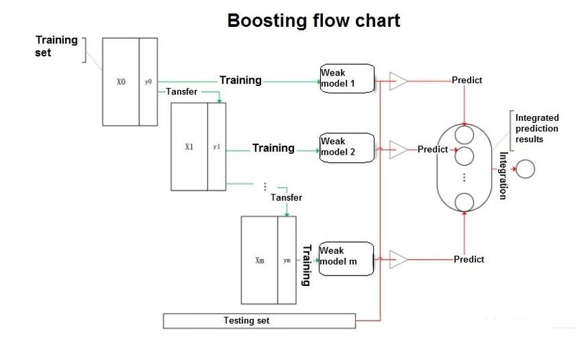
Figure 4 shows the flowchart of the Boosting algorithms, which can be broadly divided into the
following steps:

 1. To train a weak classifier using the training dataset;
 2. To adjust training dataset to allow conversion of the weak classifier using a pre-defined
 strategy;
 3. To repeat the training of other weak classifiers using the same approach (could also
 be done in parallel distributed computational process). All weak classifiers in the
 boosting can be different;
 4. To combine the weak classifiers obtained from the previous training to form a strong
 classifier; and
 5. To improve the accuracy of a given learning algorithm.

 [Insert Figure 4 here]

4.4. Measuring the Predictive Performance

The previous study has shown the superiority of the tree-based methods, which are able to
account for non-linearity in the predictive relationships, compared to the traditional multiple
regression models. However, we propose more objective ways to assess the predictive
performance of the proposed AI-AVM models using the three measures, which include R2,
Root mean square error (RMSE) and Mean absolute percentage error (MAPE), and each of
the measure is defined as follows:

 R2 = (r( Actual _ Pr ice, Pr edict _ Pr ice) )  100% (3)
 2

 N

  ( Actual _ Pr ice − Pr edict _ Pr ice )
 i i
 2

 RMSE = i =1
 (4)
 N

where N is the number of cases.

 N
 Actual _ Pr icei − Pr edict _ Pr icei
 
 i =1 Actual _ Pr icei
 MAPE =  100% (5)
 N

 11

where N is the number of cases.

R2 represents the variance of a dependent variable that is accounted for by the predictors;
and a high value means better performance. In contrast, for RMSE and MAPE, a smaller value
means better prediction accuracy. By randomly splitting the data into a training dataset and a
test dataset, the three indices are randomly derived. We repeat the estimations by 50 times
for each training-test split set to enable the convergence in the prediction accuracy. The
average R2, RMSE and MAPE are calculated to measure the model’s prediction accuracy.

5. Applications of the proposed AI-AVM

We illustrate how the proposed AI-AVM can be applied to the valuations for the private and
the public housing markets in Singapore. We use the three tree-based method to develop the
AI-AVM model. In training the model, the dataset is split into the training dataset and the testing
dataset with a ratio of 9:1. The data analyses are conducted using the algorithms written in
the R program.

The first step of developing the AI-AVM model involves data collection, cleaning and coding of
input variables, such as unit size, floor level, tenure, sale type, project name and sale date.
We also compute the average of the previous year prices at the project level, as the proxy of
historical reference market prices in the locality. From the large full sample dataset, we drop
observations with incomplete and missing data, and truncate 1% of the samples from both tail-
end distributions to eliminate outliers.

The following sections discuss the input variables, descriptive statistics, and then the
predictive results of the proposed AI-AVM.

5.1. Input variables

To test the model, we collect a total of 378,032 sample transaction data from both the private
and the public (resale) housing markets in Singapore covering the period from 1995 to 2019.
Other than the transaction unit price, which is the dependent variable in the model, we also
obtain a list of 9 hedonic property and spatial attributes that are used as the predictors in the
proposed AI-AVM model. Table 1 describes the variables.

 [Insert Table 1 here]

 12

5.2. Descriptive Statistics

Table 2 shows the descriptive statistics of mean, minimum, maximum, and standard deviation
for the dependent variables using the sample transaction data in the private and the public
housing markets, respectively. The table shows separate summary statistics for the private
and the public housing market transaction data.

 [Insert Table 2 here]

As the public (resale) housing market is a regulated market, which is only open to Singaporean
residents, the average transaction unit price of S$3,289 is lower than the average price of
S$9,656 in the private housing market in Singapore. The unit price last year is a slightly lower
both for public (S$3,169) and private housing (S$9,051). Due to the land scarcity in Singapore,
the high-rise high-density living is prevalent in both private and public housing markets, and
the average floor levels are estimated at 8.36 and 7.5, respectively. By unit size, the average
gross floor area of private housing units is bigger at 126.22 square meter (sqm) compared to
the average floor area of 96.93 sqm for public housing flats. The private housing units are
located closer to the CBD comparing the average distance of 7.3 kilometer (km) relative to
11.6 km for the public housing flats. In term of the distance to the nearest MRT stations, the
average distances are not significantly different at 1.09 km and 0.7 km for the private and the
public housing flats, respectively. The public housing shows an average age of 29.49 years,
which is older than private housing of 10.73 years. In addition, half of private housing have the
freehold tenure.

5.3. Univariate analyses

Before running the predictive tests on the proposed AI-AVM model, we run the univariate
analyses on the relationship between the predictors and the outcomes, which are the property
prices. We show the line plots of the relationship between the continuous predictors and the
property prices; and the box plots of the relationship between the categorical predictors and
the property prices. Figures 5 and 6 show separately the two different sets of line and box
plots for the private and the public (HDB) housing markets, respectively.

 [Insert Figures 5 and 6 here]

For the line plots of continuous data, the red line shows the linear fits of the data, whereas the
blue smooth line shows the actual lines for the data. For the box plots of categorical data, the

 13

vertical dots show the distribution of the observations. The plots for the private and public
housing markets show significant non-linearity in the univariate relationships in the predictors
and the outcome variables. The spatial variables, such as the distance to the closest MRT and
to the CBD, are highly non-linear, and the property attributes, such as unit size and floor level,
are also found to have non-linear relationships with property prices in both the private and the
public housing markets.

5.4. Predictive Tests of the AI-AVM

We first run the standard MRA model using the same response and the predictor variables as
described in Table 1, then apply two different version of the AI-AVM, which are the Decision
Tree and the Boosting Methods to the same dataset for both the private and the public housing
markets in Singapore. For the purposes of evaluating the predictive performance of the three
models, a simple “pseudo-horserace” based on the residuals of predictive outcomes are
compared. Table 3 shows the results of the prediction accuracy of the three methods when
applied to determine values of the transacted private and public properties, respectively. The
results are divided to two parts, the left-hand panel (I) shows the results based on the training
dataset, whereas the right-hand panel (II) shows the results based on the testing dataset.

 [Insert Table 3 here]

We first look at the top Panel A of Table 3 on the performance of the models in predicting
private property prices. The results based on the training dataset show that the MRA model
predicts about 83.38% variance of real estate unit price with an average difference of
$1,482.05 between the actual sale price and the predicted price; and the error is about 12.46%
of the sale unit price. However, the decision tree method accounts for about 79.63% variances
in property prices with an average residual error of $1,640.96, which is estimated at 13.84%
of the actual sale price. For the boosting based decision tree model, the amount variance
accounted for by the predictors is the highest at 91.33%, and the average residual error is
$1,070.86, which is smaller than the MRA and the decision tree method. The MAPE of
boosting is estimated at only 8.55%, which is also significantly smaller than the other two
models. Therefore, based on the three indices, the AI-AVM based on the boosting method
perform the best in the predictive tests, and it out-perform the traditional MRA and the standard
decision tree method. The results remain consistent when the testing dataset is used in the
predictive tests.
The lower Panel (B) shows the same predictive test results for the public housing market.
Based on the train dataset, the results show that the MRA model predicts 86.86% of the

 14

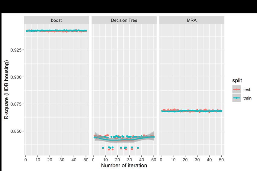
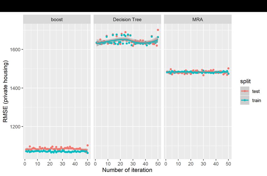
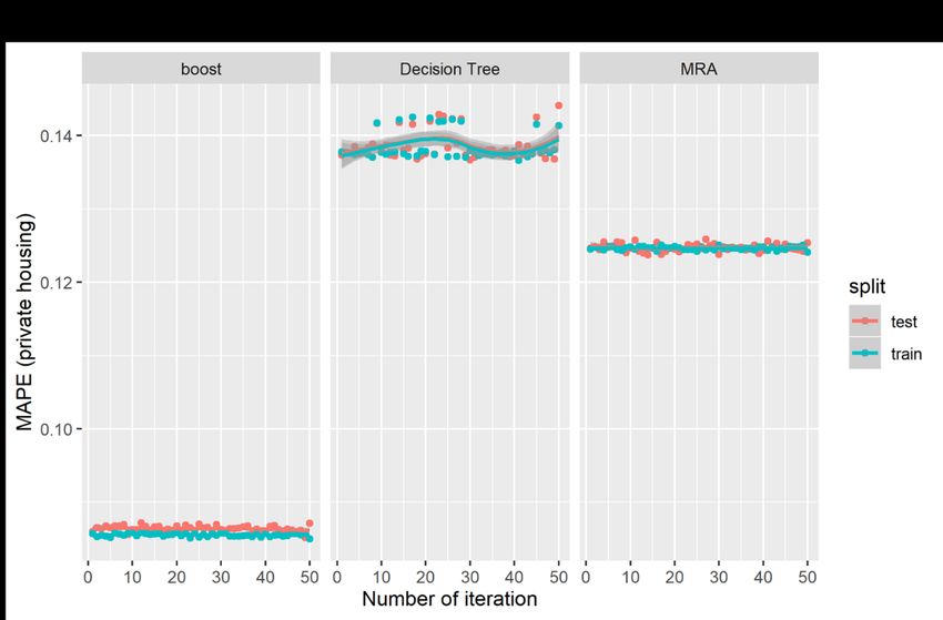
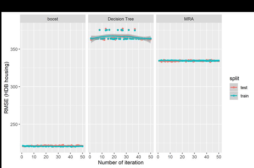
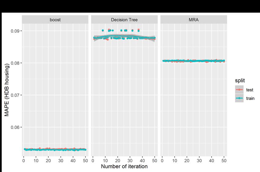
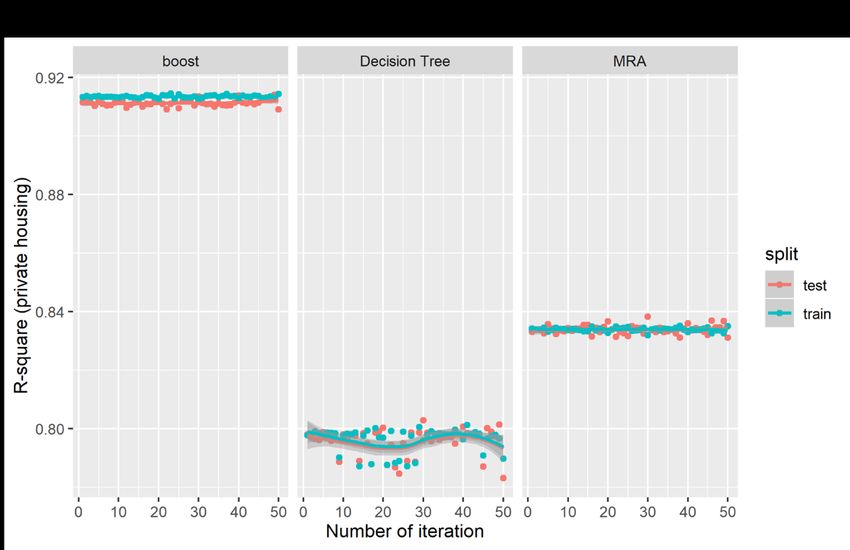
variance in public property prices, with an average difference of about $344.51 between the
predicted price and the actual sale price; and the error accounts for about 8.06% of the actual
property prices. The decision tree method has the weakest predictive performance that
accounts for only about 84.28% of the variances in prices; the average difference of about
$365.86, and the errors are estimated at on average 8.82% of the actual price. For the
boosting model, the predictive accuracy increases significantly accounting for 94.28% the
variance in prices, on average. The average difference between the predicted price and the
actual price also decreases significantly to $220.71, which is estimated at 5.30% of the actual
price. The results again affirm the predictive power of the boosting model, which are much
superior than the traditional MRA model and the decision tree model in predicting public (HDB)
housing prices.

Figures 7 and 8 show the graphical plots of the three performance indicators estimated based
on 50 random iterations in the predictions of private property prices. Figures 7(a), 7(b) and 7(c)
show the distributions for the R2, RMSE and MAPE, respectively, for the private property prices;
and Figure 8(a), 8(b) and 8(c) show the corresponding distributions for the three predictive
indicators for the public housing prices. The results are consistent with those presented in
Table 3 but are presented in the visual form. The results show that the boosting models have
the higher R2, but lower figures in both the RMSE and MAPE. However, the results show
significant fluctuations in distributions in the two AI-based models relative to the MRA model,
which shows more stable results in the iterations.

 [Insert Figures 7 and 8 here]

We run the out-of-sample tests using the housing transactions in 2018, which are not included
in the training dataset covering only data from 1995 to 2017. We compare the out-of-sample
predictions of the AI-AVM (boosting) model and also use the enhanced spatially-adjusted MRA
model for private housing in Figure 9 and public housing in Figure 10. The results the AI-AVM
model could keep the predictive errors (red dots) within a very tight range of less than 25% for
majority of private housing (with an average of 8.41%) and 20% for majority of public housing
(with an average of 5.62%). The enhanced MRA model seems to perform better after adjusting
for spatial variations in the MRA models.2 However, in term of distributions of the predictive
errors, the AI-AVM model appears to be more consistent and stable in the prediction as
indicated by tighter distributions of the predictive error terms.

2 The discussions of the spatially adjusted MRA is not within the scope of the current study, and the details are
 available in the paper by Agarwal, Fan, Sing and McMillen (2019).

 15

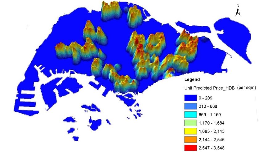
[Insert Figure 9 here]
 [Insert Figure 10 here]

Apparently, price history (Pyp), which is the taverage transaction unit price of the same project
in the previous one year), timing (year), and geographic location (distance to CBD) are the top
three crucial variables in determining housing price for both private and HDB market. Some
variables like area, month, and floor played less important role in predicting the property price.
Other factors like age and distance to MRT is not influential in calculating the apartment price
in our model.

 [Insert Figure 11 here]
 [Insert Figure 12 here]

5.5. Potential Applications

In a study by Agarwal et al (2019), the AI-AVM model has been used to estimate values of
houses for the entire household in Singapore, where in the study they matched housing
address to other personal data. They track inter-generational housing mobility in Singapore,
where they show how about Singaporean families have experience an upward mobility in
housing wealth. They showed that children born to the lower 60% percentile of the families by
housing wealth have moved up in their housing ladders relative to their parent generations.
The upward mobility indicates the successful social engineering and the public housing
programme in Singapore that help more families to own their houses at affordable prices.

We illustrate how we could also apply the AI-AVM to determine flat values of 816,544
households living in public housing flats in Singapore. We collected the data from a proprietary
source of data that contain personal information, housing address and housing attributes of
each of the sample households. The public housing flats cover about 80% of the housing
stocks in Singapore. It would be a daunting task for the Inland Revenue Authority of Singapore
(IRAS) to assess the values for all these housing flats for property tax purposes. We use the
trained data from our resale transaction records to develop an AI-AVM model, and use the
model to automatically value all the 816,544 housing flats based on the key attributes like the
unit size, floor level, building age, and the spatial measures, such as distance to the nearest
MRT station and distance to the CBD.

The summary statistics of the full sample of public housing flats estimated based on the

 16

proposed AI-AVM models are summarized in Table 4. The results show that the average unit
value for public housing flat is estimated at S$3,529.11 per square meter (psm). Based on an
average unit size of 78.24 square meter, the average public housing value is estimated at
S$276,130.4, as in the estimation date in 2019. The average floor height of 7.4 storey indicates
the high-rise and high-density nature of public housing in Singapore; and the average building
age of the sample is 22.96.

 [Insert Table 4 here]

Due to unavailability of the income data at the household level, we are not able to merge the
estimated public housing value data to derive housing wealth of individual households in
Singapore. However, the assessment of housing values could be very useful for property tax
assessment purposes. Based on the estimated values, we created a 3-dimensional heat map
of housing values in Figure 13. The value heat map shows prices are distributed spatially
across the island with different peaks in selected neighbourhoods. Due to the deliberate public
housing policies in Singapore to build new towns across the island, we do not see peak prices
to be concentrated only in one location, and the prices are distributed quite widely and evenly
across different parts of Singapore.

 [Insert Figure 13 here]

By sorting the housing flats based on the postal district (the first 2-digit of the postal code), we
could see examine heterogeneity in unit prices in different neighbourhoods. The districts with
the highest average housing values are found in postal districts 21 (Little India, Farrer Park,
Jalan Besar, Lavender), 10 (Telok Blangah, Harbourfront), 31 (Balestier, Toa Payoh,
Serangoon) and 39 (Geylang, Eunos); where the district 10 is the area where the tallest public
housing flats, Pinnacle @ Duxton are built on a redeveloped site. We also identify the postal
districts with the lowest average public housing values, which are in districts 50 (Loyang,
Changi), 26 (Bukit Timah, Holland Road), 73 (Kranji, Woodgrove, Woodlands), and 68
(Hillview, Dairy Farm, Bukit Panjang, Chao Chu Kang). District 26 is the traditional prime
private residential area, and the limited supply of public housing flats in the area could explain
the relative low average values of public housing in the district.

6. Conclusion

This study develops the machine learning approach, or more specifically the tree-based
method, for the valuation of the private and the public housing units in Singapore. Two tree-

 17

based methods, which are the decision tree and the boosting, are used to develop the
proposed AI-AVM models. For the purpose of determining the prediction accuracy of the
models, we conduct a “horserace” of the two AI-AVM models in relation to the traditional MRA
model using a set of real estate transaction data for the period from 1995 to 2018.

The boosting model of the AI-AVM outperform the decision tree and the MRA model in the
predicting tests for both the private and the public housing markets. When using the testing
dataset, the variance of up to 91% in the private market, and 94% in the public housing market
can be predicted by the boosting model. Public housing units that have more homogenous
property attributes relative to private housing units could explain the differential performance
of the boosting models when applied predict prices in the two markets. Despite the differences,
the errors of the boosting model is kept within relative small MAPE of not more than 9% when
predicting housing values using the boosting method. The predictive test results show that the
AI-boosting model, is more superior than the traditional MRA model when used to develop
AVM model to predict housing values in both the private and the public housing markets.

Although the models are developed based on the housing datasets in Singapore, the proposed
AI-AVM models could be easily adapted and applied for automated valuations in other real
estate markets. Compared to the earlier studies on AI-AVM, the study has two distinctive
features in the AI applications to property valuations: First, the boosting method, which is a
more robust and powerful algorithm relative to the more conventional AI models, such as
backpropagation model, etc, has been used; and the model that allows for inter-dependence
in the tree structure significantly improve the predictive power of the model; and Second, unlike
the earlier attempt to train the AI models using smaller sample data, this study uses more than
300,000 transaction data with a large set of attributes to train the model, and the effects are
more apparent in term of smaller predictive errors and better out-of-sample forecasting
performance.

We could further augment and expand the predictive powers of the proposed AI-AVM by
exploring other algorithm such as random forest, etc in the future study to predict housing
prices. Other future extensions include using the AI-AVM to predict commercial property
values, which are dependent on the future cash flows that are highly serially correlated; and
to improve the computation efficiency of the model by allowing other fuzzy definitions for
selected property attributes in the models.

 18

Reference:
Agarwal, Sumit, Yi Fan, Wenlan Qian, Tien Foo Sing (2019). Like Father Like Son? Social
Engineering and Intergenerational Housing Wealth Mobility. Working paper, Institute of Real
Estate and Urban Studies, National University of Singapore.
Allen, W.C., & Zumalt, J.K. (1994). Neural networks: A word of caution. Unpublished working
paper, Colorado State University.
Bebchuk, L. A., Cohen, A., & Spamann, H. (2010). The wages of failure: Executive
compensation at Bear Stears and Lehman 2000–2008. Yale Journal on Regulation,
27(2), 257–282
Borst, R.A. (1992). Artificial neural networks: The next modelling/calibration technology for
the assessment community. Artificial Neural Networks, 69-94.
Byrne, P. (1995). Fuzzy analysis: A vague way of dealing with uncertainty in real estate
analysis. Journal of Property Valuation & Investment, 13(3), 22-41.
Chiarazzo V., Caggiani, L., & Marinelli, M. (2014). A Neural Network based Model for Real
Estate Price Estimation Considering Environmental Quality of Property Location.
Transportation Research Procedia, 3, 810-817.
Do, A.Q., & Grudnitski, G. (1992). A neural network approach to residential property
appraisal. The Real Estate Appraiser, 58, 38-45.
Evans, A., James, H., & Collins, A. (1992). Artificial neural networks: An application to
residential valuation in the UK. Journal of Property valuation & Investment, 11, 195f-204.
Glumac Brano & Des Rosiers François, 2018. "Real estate and land property automated
valuation systems: A taxonomy and conceptual model," LISER Working Paper Series 2018-
09, LISER.
Gongzlez, M.A.S., & Formoso, C.T. (2006). Mass appraisal with genetic fuzzy rule-based
systems. Property Management, 24(1), 20-30.
Sucharita Gopal. (1998) Artificial Neural Networks for Spatial Data Analysis, NCGIA Core
Curriculum in GIScience, http://www.ncgia.ucsb.edu/giscc/units/u188/u188.html posted
December 22, 1998.
Guan, J. & Levitan, A.S. (1997). Artificial neural network based assessment of residential
real estate property prices: A case study. Accounting Forum, 20(3/4), 311-326.
Guan, J., Zurada, J., & Lavitan, A.S. (2008). An Adaptive Neuro-Fuzzy Inference System
based approach to real estate property assessment. Journal of Real Estate Research, 30(4),
395-422.
Gwartney, 1970. T.A. Gwartney Computerized assessment program. D.M. Holland (Ed.), The
Assessment of Land Value, Univ. of Wisconsin Press, Milwaukee.
Hawley, D., Johnson, J.D., & Raina, D. (1990). Artificial neural systems; A new tool for
financial decision-making. Financial Analyst Journal, 46(6), 63-72.
Hopfield, J.J. (1982). Neural networks and physical systems with emergent collective
computational abilities. Proceedings of the National Academy of Sciences, 79, 2554-2558.
Huang, C.S., Dorsey, R.E., & Boose, M.A. (1994). Life insurer financial distress prediction:
neural network model. Journal of Insurance Regulation, 13(2), 131-167.

 19

Ibrahim, M.F., Cheng, F.J. & Eng, K.H. (2005). Automated valuation model: an application to
the public housing resale market in Singapore. Property Management, 23, 357-373
James, G., Witten, D., Hastie, T., & Tibshirani, R. (2013). An introduction to statistical
learning with applications in R. Springer, New York.
Kryzanowski, L., Galler, M., & Wright, D.W. (1993). Using artificial neural networks to pick
stocks. Financial Analyst Journal, 49(4), 21-27.
Lenk, M.M., Worzala, E.M., & Silva, A. (1997). High-tech valuation: Should artificial neural
networks bypass the human valuers? Journal of Property Valuation & Investment, 15(1), 8-
26.
Li Q., Meng, Q., & Cai, J. (2009). Predicting hourly cooling load in the building: A comparison
of support vector machine and different artificial neural networks. Energy Conversion &
Management, 50(1), 90-96.
McClelland, J.L., & Rumelhart, D.E. (1986). Parallel distributed processing: Explorations in
the microstructure of cognition, Vol (1): Foundation. MIT Press, Cambridge M.A.
McClelland, J.L., & Rumelhart, D.E. (1988). Explorations in parallel distributed processing: A
handbook of models, programs, and exercises. MIT Press, Cambridge M.A.
McCluskey, W.J. (1996). Predictive accuracy of machine learning models for the mass
appraisal of residential property. New Zealand Valuers’ Journal, 41-7.
McCluskey, W., Deddis, W., Mannis, A., McBurney, D., & Borst, R. (1997). Interactive
application of computer assisted mass appraisal and geographic information systems.
Journal of Property Valuation and Investment, 15(5), 448-465.
McGreal, S., Adair, A., McBurney, D., & Patterson, D. (1998). Neural networks: The
prediction of residential values. Journal of Property Valuation & Investment, 16(1), 57-70.
Minsky, M., & Papert, S. (1969). Perceptrons, MIT Press, Cambridge, M.A.
Nawawi, A.H., Jenkins, D., & Gronow, S. (1997). Expert system development for the mass
appraisal of commercial property in Malaysia. Journal of the Society of Surveying Technicians,
18(8), 66-72.
Nguyen, N., & Cripps, A. (2001). Predicting housing value: A comparison of multiple
regression analysis and artificial neural networks. Journal of Real Estate Research, 22(3),
313-336.
O’Roarty, B., Patterson, D., McGreal, W.S., & Adair, A.S. (1997). A case based reasoning
approach to the selection of comparable evidence for retail rent determination. Expert
Systems with Applications, 12(4), 417-428.
Pagourtzi E, Assimakopoulos, V., & Hatzichristos, T. (2003). Real estate appraisal: A review
of valuation methods. Journal of Property Investment & Finance, 21(4), 383-401.
Peterson S., & Flanagan, A.B. (2009). Neural Network Hedonic Pricing Models in Mass Real
Estate Appraisal. Journal of Real Estate Research, 31(2), 147-164.
Rosenblatt, F. (1958). The Perceptron: A probabilistic mnodel for information storage and
organization in the brain. Psychological Review, 65, 386-408.
Rossini, P.A. (1997). Artificial neural networks versus multiple regression in the valuation of
residential property. Australian Land Economics Review, 3, 1-12.

 20

Ruppert D. (2004). The Elements of Statistical Learning: Data Mining, Inference, and
Prediction. Publications of the American Statistical Association, 99(466), 1.
Sarip, A. G. (2005, January 23–27). Integrating artificial neural networks and GIS for single-
property valuation. Proceedings of the 11th Pacific Rim Property Research Conference,
Melbourne (pp. 1–16).

Sing, T.F., Ho, K.H.D., & Tay, P.H. (2002). A Fuzzy Discounted Cash Flow Analysis for Real
Estate Investment, in Wang, K and Wolverton, Marvin L. (Editors), Real Estate Valuation
Theory.

Tay, D.P.H., & Ho, D.K.H. (1992). Artificial intelligence and the mass appraisal of residential
apartments. Journal of Property Valuation and Investment, 10(2), 525-539.
Trippi, R.R., & Turban, E. (1993). Neural Networks in Finance and Investing. Chicago,
Probus Publishing.
Tsukuda, J., & Baba, S.I. (1994). Predicting Japanese corporate bankruptcy in terms of
financial data using neural networks. Computers & Industrial Engineering, 27(1-4), 445-448.
Wong, F.S., Wang, P.Z., Goh, T.H., & Quek, B.K. (1992). Fuzzy neural systems for stock
selection. Financial Analyst Journal, 48(1), 47-52.
Worzala, E., Lenk, M., & Silva, A. (1995). An exploration of neural networks and its
application to real estate valuation. Journal of Real Estate Research, 10(2), 185-201.
Rossini, 1997;
Zurada, J., Levitan, A.S., & Guan, J. (2011). A comparison of regression and artificial
intelligence methods in a mass appraisal; context. Journal of Real Estate Research, 33(3),
349-387.

 21

Table1 Description of variables

For private housing model
Variable Description
Uprice transacted unit price;
Floor Floor level (height) of property;
Area Unit size (square meters);
Month The month in the transaction date, [1, 2, …12];
Year The year of the transaction, [1995 to 2019];
 Land tenure, 1 for freehold and lease >900 years; 0 otherwise; only
Freehold
 for private housing
Dist_city Distance to the CBD (km);
Dist_MRT Distance to the nearest MRT station (in km);
 The average transaction unit price of the same project in the
Pyp
 previous one year

For HDB model
Variable Description
Uprice transacted unit price;
Floor Floor level (height) of property;
Area Unit size (square meters);
Month The month in the transaction date, [1, 2, …12];
Year The year of the transaction, [1995 to 2019];
Dist_city Distance to the CBD (km);
Dist_MRT Distance to the nearest MRT station (in km);
 The average transaction unit price of the same project in the
Pyp
 previous one year

 22

Table 2: Descriptive Statistics

 variable mean min max SD
 HDB uprice 3288.71 1963.41 5462.69 927.33
 Housing floor 7.5 2 38 4.41
 Market area 96.93 31 280 25.25
 age 29.49 5 52 9.33
 year 2007.97 2001 2017 4.57
 month 6.46 1 12 3.4
 dist_MRT 0.7 0.01 2.81 0.46
 dist_city 11.6 1.4 18.4 3.86
 Pyp 3168.5 1963.77 5462.69 866.05
 Private uprice 9655.64 3965.52 27133.33 3720.12
 Housing floor 8.36 1 66 6.78
 Market area 126.22 24 1212 53.26
 age 10.73 1 64 7.29
 freehold 0.49 0 1 0.5
 year 2009.56 1996 2019 5.65
 month 6.22 1 12 3.18
 dist_MRT 1.09 0.03 5.75 0.78
 dist_city 7.3 0.4 24.4 3.9
 Pyp 9051.13 3965.52 19658.11 3601.59

 23

Table 3 Prediction accuracy of three methods

 train test
 R2 RMSE MAPE R2 RMSE MAPE
 Private MRA 83.38% 1482.05 12.46% 83.38% 1482.31 12.47%
 Housing Decision Tree 79.63% 1640.96 13.84% 79.56% 1643.90 13.86%
 Market Boosting 91.33% 1070.86 8.55% 91.12% 1083.96 8.64%
 HDB MRA 86.86% 334.51 8.06% 86.87% 334.34 8.06%
 Housing Decision Tree 84.28% 365.86 8.82% 84.27% 365.98 8.82%
 Market Boosting 94.28% 220.71 5.30% 94.25% 221.22 5.31%

Table 4: Assessing Values for Public Housing Flats

 Variable Symbol Mean Std. Dev. Min Max
 Unit Price (S$/psm) price 3529.114 990.953 1919.020 5872.630
 Floor Level (storey) floor 7.405 3.989 1.000 30.000
 Unit Size (sqm) area 78.244 20.821 40.500 161.000
 Building age age 22.964 8.052 3.000 48.000
 Distance to MRT dist_mrt 6.229 3.358 0.200 31.790
 Distance to CBD dist_city 12.815 4.613 1.660 21.880

 24

Figure 1: ANN Model and 3 Interconnected Layers
 Figure 1: ANN Model with 3 Layers

 Source: Sarip, 2019

 25

Figure 2: ANN Property Valuation Model
 Figure 2: ANN Property Valuation Model

 Source: Sarip, 2019

 26

Figure 3 The decision tree method
 Figure 1 Decision Tree Method

 (Source: Ruppert, 2004)

 27

Figure 4 The in-house designed Boosting Model
Figure 2

 28

Figure 5 Univariate Plots of Response and Predictors for Private Housing Market

 29

Figure 6 Univariate Analyses of Response and Predictors for HDB Housing Market

 30

Figure 7 Predictive Performance Tests for Private Housing Markert

 31

Figure 8 Predictive Performance Tests for HDB Housing Market

 32

33

Figure 9 Out-of-Sample Forecasting Tests for Private Housing

 34

Figure 10 Out-of-Sample Forecasting Tests for HDB

 35

Figure 11 The importance of predictors for private housing price

 Pyp
 year
 dist_city
 area
 month
 floor
 freehold
 age
 dist_MRT

 0 20 40 60 80 100
 Relative Influence

Figure 12 The importance of predictors for HDB housing price

 Pyp

 year

 dist_city

 area

 floor

 month

 age

 dist_MRT

 0 10 20 30 40 50 60 70 80
 Relative Influence

 36

Figure 13: 3-Dimensional Housing Value Heatmap for Public Housing Flats in Singapore
 (Based on S$ per square meter)

 37