Using Human Ratings for Feedback Control: A Supervised Learning Approach with Application to Rehabilitation Robotics
←
→
Page content transcription
If your browser does not render page correctly, please read the page content below
Using Human Ratings for Feedback Control: A Supervised Learning
                                                Approach with Application to Rehabilitation Robotics
                                                                Marcel Menner, Lukas Neuner, Lars Lünenburger, and Melanie N. Zeilinger

                                            Abstract—This paper presents a method for tailoring a para-          method addresses general human-in-the-loop scenarios, where
                                         metric controller based on human ratings. The method leverages          expert knowledge can improve system operation.
                                         supervised learning concepts in order to train a reward model
                                         from data. It is applied to a gait rehabilitation robot with the
                                                                                                                    In this paper, we propose a two-step approach to achieve
                                         goal of teaching the robot how to walk patients physiologically. In     automatic input adaptations: First, we define a feature vector
                                         this context, the reward model judges the physiology of the gait        to characterize the gait cycle and postulate a reward model
arXiv:1906.09847v1 [cs.RO] 24 Jun 2019

                                         cycle (instead of therapists) using sensor measurements provided        to judge the physiology of the gait cycle using the feature
                                         by the robot and the automatic feedback controller chooses the          vector. The reward model is trained with therapists’ ratings
                                         input settings of the robot so as to maximize the reward. The
                                         key advantage of the proposed method is that only a few input
                                                                                                                 using a supervised learning technique, where the feature vector
                                         adaptations are necessary to achieve a physiological gait cycle.        is obtained from sensor measurements provided by the robot.
                                         Experiments with non-disabled subjects show that the proposed           The sensor measurements are the angle, torque, and power of
                                         method permits the incorporation of human expertise into a              both the hip and knee joints of the robot. Second, we use the
                                         control law and to automatically walk patients physiologically.         gradient of the reward model to determine input adaptations
                                                                                                                 that achieve the desired gait cycle. This involves a steady-state
                                           Index Terms—Learning and Adaptive Systems, Human Feed-                model to relate the gradient of the reward model with respect
                                         back-based Control, Rehabilitation Robotics, Human-Centered             to the feature vector (high dimensional) to input settings (low
                                         Robotics.
                                                                                                                 dimensional) that adjust the gait cycle. A key component in
                                                                                                                 the proposed formulation is that the reward model and its
                                                                I. I NTRODUCTION                                 gradient are formulated as functions of the feature vector rather
                                            Humans can perform very complex tasks that are difficult to          than the input settings. The high dimensionality of the feature
                                         achieve with autonomous systems. The dependency on human                vector allows us to use one model for all human subjects with
                                         supervision or expertise still restricts efficient operation of         very different body types, which enables very efficient online
                                         many complex systems. An important domain where human                   application of the proposed method. In order to train both
                                         expertise is usually needed is rehabilitation robotics, where           the reward model and the steady-state model, we collected
                                         we consider the robot-assisted gait trainer Lokomat® [1] in             data with various physiological and non-physiological input
                                         this paper, see Figure 1. Robotic systems like the Lokomat              settings from 16 non-disabled subjects. The subjects were
                                         have recently been introduced in gait rehabilitation following          instructed to be passive while being walked by the robot
                                         neurological injuries with the goal of mitigating the limita-           in order to imitate patients with limited or no ability to
                                         tions of conventional therapy [2]–[6]. However, training with           walk in the early stages of recovery. Experiments with ten
                                         such robots still requires the supervision and interaction of           non-disabled subjects highlighted the ability of the proposed
                                         experienced therapists [1].                                             method to improve the walking pattern within few adaptations
                                            Gait rehabilitation with the Lokomat currently requires              starting from multiple initially non-physiological gait cycles.
                                         physiotherapists to manually adjust the mechanical setup and
                                         input settings, e.g. the speed of the treadmill or the range of
                                         motion, in order to bring patients into a physiological and safe
                                         gait cycle. Therapists have to be trained specifically for the
                                         device and acquire substantial experience in order to achieve
                                         good input settings. Although there are guidelines for their
                                         adjustments [7], it remains a heuristic process, which strongly
                                         depends on the knowledge and experience of the therapist.
                                         Automatic adaptation of input settings can reduce the duration
                                         of therapists’ schooling, improve patient training, make the
                                         technology more broadly applicable, and can be more cost
                                         effective. In this work, we propose a method to automatically
                                         adapt input settings. Although the motivation behind this
                                         work is in the domain of rehabilitation robotics, the proposed
                                           M. Menner, L. Neuner, and M.N. Zeilinger are with the Institute for
                                         Dynamic Systems and Control, ETH Zurich, 8092 Zurich, Switzerland
                                         {mmenner,lneuner,mzeilinger}@ethz.ch                                    Fig. 1. Lokomat® gait rehabilitation robot (Hocoma AG, Volketswil, CH).
                                           L. Lünenburger is with Hocoma AG, 8604 Volketswil, Switzerland
                                         lars.luenenburger@hocoma.com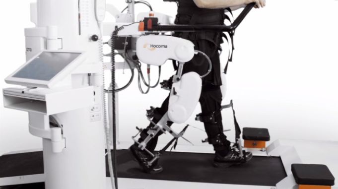
Related Work                                                        with a bodyweight support system, it provides controlled
   Adaptive control strategies have been the subject of a           flexion and extension movements of the hip and knee joints
body of research in robotic gait trainers with the goal of          in the sagittal plane. Leg motions are repeated based on
improving the therapeutic outcome of treadmill training [8]–        predefined but adjustable reference trajectories. Additional
[13]. The work in [8] presents multiple strategies for automatic    passive foot lifters ensure ankle dorsiflexion during swing.
gait cycle adaptation in robot-aided gait rehabilitation based      The bodyweight support system partially relieves patients from
on minimizing the interaction torques between device and            their bodyweight via an attached harness. A user interface
patient. Biomechanical recordings to provide feedback about a       enables gait cycle adjustments by therapists via a number of
patient’s activity level are introduced in [9], [10]. Automated     input settings [1], [10].
synchronization between treadmill and orthosis based on it-            Input Settings: One important task of the therapist operating
erative learning is introduced in [11]. In [12], a path control     the Lokomat is the adjustment of the input settings to obtain
method is introduced to allow voluntary movements along a           a desirable gait trajectory. A total of 13 input settings can be
physiological path defined by a virtual tunnel. An algorithm to     adjusted to affect the walking behavior, which are introduced
adjust the mechanical impedance of an orthosis joint based on       in Table I. In this work, we propose a method that can
the level of support required by a patient is proposed in [13].     automate or assist the therapists in the adjustment of the input
Further research in the domain of rehabilitation robotics is        settings by measuring the gait cycle.
presented, e.g., in [14], [15]. In [14], the human motor system
                                                                                                   TABLE I
is modeled and analyzed as approximating an optimization                              I NPUT S ETTINGS OF THE L OKOMAT
problem trading off effort and kinematic error. In [15], a
patient’s psychological state is estimated to judge their mental     Input Setting & Description               Step-size     Range
engagement.                                                          Hip Range of Motion (Left & Right)        3◦            23◦ , 59◦
                                                                     Defines the amount of flexion and extension
   Related fields are gait cycle classification [16]–[19], rein-
                                                                     Hip Offset (Left & Right)                 1◦            -5◦ , 10◦
forcement learning from human feedback [20]–[27], or inverse         Shifts movements towards extension or flexion
learning methods [28]–[41]. Differing from gait cycle classifi-      Knee Range of Motion (Left & Right)       3◦            32◦ , 77◦
cation methods [16]–[19], this paper does not aim to identify        Defines amount of flexion
                                                                     Knee Offset (Left & Right)                1◦            0◦ , 8◦
a human’s individual gait but to generalize the classification
                                                                     Shifts movement into flexion for hyperextension correction
of a physiological gait using data from multiple humans.             Speed                                     0.1km/h       0.5km/h, 3km/h
Further, we infer the physiology of the gait from data and use       Sets the treadmill speed
the gathered knowledge for feedback control. Reinforcement           Orthosis speed                            0.01          0.15, 0.8
learning uses a trial and error search to find a control policy      Defines the orthosis and affects walking cadence
                                                                     Bodyweight Support                        continuous    0kg, 85kg
[42]. The framework proposed in [20] allows human trainers to        Defines carried weight for unloading
shape a policy using approval or disapproval. In [21], human-        Guidance Force                            5%            0%, 100%
generated rewards within a reinforcement learning framework          Sets amount of assistance
are employed to control a 2-joint velocity control task. In [22],    Pelvic                                    1cm           0cm, 4cm
                                                                     Defines lateral movement
human feedback is not used as a reward signal but utilized as
a direct policy label. In [23], human preferences are learned
though ratings based on a pairwise comparison of trajectories.
In [24], a robot motion planning problem is considered, where       A. State-of-the-Art Therapy Session
users provide a ranking of paths that enable the evaluation            The current practice of gait rehabilitation with the Lokomat
of the importance of different constraints. In [25], a method       includes the preparation and setup of the patient and device,
is presented that actively synthesizes queries to a user to         actual gait training, and finally removing the patient from the
update a distribution over reward parameters. In [26], user         system [7]. Gait training is further divided into three phases:
preferences in a traffic scenario are learned based on human
                                                                    1. Safe walk: The patient is gradually lowered until the
guidance in terms of feature queries. In [27], human ratings
                                                                        dynamic range for bodyweight support is reached. The
are used to learn a probabilistic Markov model. However, the
                                                                        purpose of this first phase is to ensure a safe and non-
online application of these methods typically requires a few
                                                                        harmful gait cycle.
hundred human ratings to learn a policy. This is infeasible
                                                                    2. Physiological walk: After ensuring safe movements, the
when working with a patient, where a comparatively small
                                                                        gait cycle is adjusted so that the patient is walked phys-
number of feedback rounds has to be sufficient. In inverse
                                                                        iologically by the robot.
reinforcement learning [28]–[34] and inverse optimal control
                                                                    3. Goal-oriented walk: The gait cycle is adjusted to achieve
[35]–[41], demonstrations from humans are utilized to learn a
                                                                        therapy goals for individual sessions while ensuring that
reward/objective function instead of ratings.
                                                                        the patient’s gait remains physiological.
                                                                       In this paper, we focus on the physiological walk. In a state-
  II. H ARDWARE D ESCRIPTION & P ROBLEM D EFINITION                 of-the-art therapy session, therapists are advised to follow pub-
   The Lokomat® gait rehabilitation robot (Hocoma AG,               lished heuristic guidelines on how to adjust the input settings
Volketswil, CH) is a bilaterally driven gait orthosis that is       based on observations in order to reach a physiological walk.
attached to the patient’s legs by Velcro straps. In conjunction     Three examples of the heuristic guidelines are as follows: If
the step length does not match walking speed, then the hip Control Law and Conceptual Idea: The method is based on
range of motion or treadmill speed should be adjusted; if the a reward model, reflecting the control objective, and a steady-
initial contact is too late, then hip offset or the hip range state model, associating a feature vector with an input setting.
of motion should be decreased; if the foot is slipping, then The reward model is a function that assigns a scalar value to
the synchronization should be increased or the knee range of the feature vector estimating an expert rating of the ’goodness’
motion decreased. An extended overview of heuristics can be of the feature vector. The reward thereby provides a direction
found in [7]. This heuristic approach requires experience and of improvement for the feature vector, which is mapped to a
training with experts, which incurs high costs and limits the change in input settings via the steady-state model.
availability of the rehabilitation robot due to the small number We define the control law in terms of input adaptations ∆s:
of experienced experts. The proposed method aims to alleviate
this limitation as described in the following. ∆s = f −1 (α∆x + x) − s,
B. Technological Contribution where ∆x is the direction of improvement, f −1 : Rn → Rm
We propose a method for automatically suggesting suitable is the steady-state model (the inverse mapping of f (·) in (1)),
input settings for the Lokomat based on available sensor and α > 0 is the gain of the control law. We compute ∆x as
measurements in order to walk patients physiologically. The the gradient of the reward model r(x) ∈ R, i.e.
proposed framework can be used for recommending input
∆x = ∇x r(x).
settings for therapists, automatic adaptation of input settings,
or as an assistive method for therapists during schooling with Figure 3 shows an example of a reward model and indicates
the Lokomat. Figure 2 illustrates the proposed method as how its gradient is used for feedback control using the steady-
a recommendation system. The method is derived assuming state model. Both models r(x) and f −1 (·) are inferred from
that the mechanical setup of the Lokomat is done properly, data. In order to train the reward model, we utilize ratings
such that the purpose of adapting the input settings is the on an integer scale as samples of the reward model, i.e. ri =
improvement of the gait cycle and not corrections due to an 1, ...S, where ri = 1 is the worst and ri = S is the best rating.
incorrect setup. Additionally, we train a steady-state model f −1 (·) to relate the
direction of improvement suggested by the reward model to
Novel Technology
the corresponding input adaptation (bottom part of Figure 3).
Recommender input Lokomat In order to build both the reward model and the steady-state
settings
0
model, N training samples are collected. Each training sample
-10
observation
measurements
b2 ∇x r(x)
Fig. 2. Overview of the proposed method as a recommendation system. The b1
novel technology (dashed lines) augments the state-of-the-art control loop of a
therapist and the Lokomat. Sensor measurements of angle, torque, and power
of both hip and knee joints provided by the Lokomat are used to compute
recommendations for the input adaptations.
III. C ONTROLLER D ESIGN BASED ON H UMAN R ATINGS
This section describes the proposed human feedback-based
controller. In the setup considered, input settings s ∈ Rm of x2
the controlled system lead to a gait cycle represented by a x1
feature vector x ∈ Rn in steady-state:
x2 s2
x = f (s), (1)
where f is an unknown function. For the application con- x + ∆x s + ∆s
f −1
sidered, the input settings s are given in Table I and the ∆x ∆s
x s
feature vector x is composed of the statistical features of
measurements, which characterize the gait cycle and are x1 s1
further discussed in Section IV. Here, the notion of a steady-
state means that any transients due to an input adaptation have Fig. 3. Top: Example of reward model with gradient vector ∇x r(x) where
x = [x1 x2 ]T and projected level sets onto the x1 − x2 plane. The example
faded. The control objective is to find input settings s? for shows a case of three ratings ri = 1, 2, 3 separated by two classification
which x? = f (s? ) represents a desired system state, i.e. a boundaries indicated as solid black and dashed black ellipses. Bottom: steady-
physiological gait cycle in the considered application. state model to compute ∆s from ∆x where s = [s1 s2 ]T .with index i consists of a feature vector xi , the input settings closely related to a Support Vector Machine, cf. [43], with
si , and the corresponding rating ri ∈ {1, ..., S}: a polynomial kernel function of degree two. The functions
rl (x) correspond to S − 1 classification boundaries in a multi-
{xi , si , ri }N
i=1 . (2)
category classification framework. The parameters W , w,
Note that throughout this paper, the feature vector x is and b of the reward model (3) are computed by solving the
normalized using collected data xi such that the collected following optimization problem:
data are zero-mean with unit-variance in order to account for S−1
XX N
different value ranges and units, cf. [43]. minimize ξil + λ1 · kW k1 + λ2 · kwk1
Outline: The reward model is trained with the feature W ,bl ,b,ξil
l=1 i=1
vector xi and its corresponding rating ri in (2) using a subject to yil rl (xi ) ≥ 1 − ξil
∀ i = 1, ...N
supervised learning technique (Section III-A). The resulting
ξil ≥ 0 ∀ l = 1, ...S − 1 (5)
reward model is then used to compute the gradient ∇x r(x)
as direction of improvement. Finally, a steady-state model rl (xi ) = 0.5xT
i W xi + wT xi + bl
relates this direction of improvement with necessary changes l
b = b − l − 0.5
in input settings s. The steady-state model is computed using
W = WT ≺ 0
a regression technique (Section III-B).
where λ1 , λ2 > 0 control the trade-off between minimizing
A. Reward Model using Supervised Learning the training error
Pn andPmodel complexity captured by the
n
norm kW k1 = j=1 k=1 |Wjk | (elementwise 1-norm) and
The first step of the framework is the learning of a reward kwk1 , which is generally applied to avoid overfitting of a
model reflecting the physiology of the gait based on supervised model and is sometimes also called lasso regularization [43].
learning techniques [43]. The reward model is a continuous
function, i.e. it provides a reward for all x, whereas observa-
tions xi are potentially sparse. B. Feedback Control using Reward Model
In view of the considered application, we postulate a reward The second step of the proposed framework is to exploit
model of the form: the trained reward model for feedback control. The idea is
(i) to use the gradient of the reward model as the direction
r(x) = 0.5xT W x + wT x + b, (3)
of improvement and (ii) to relate this gradient to a desired
where W = W T ≺ 0, w ∈ Rn , and b ∈ R are the change in inputs with a steady-state model.
parameters to be learned from expert ratings given in the form (i) Gradient of reward model: The gradient of the inferred
of integers on a scale from 1 to S. The rationale for selecting reward model is the direction of best improvement. The control
a quadratic model with negative definite W is the observation strategy is to follow this gradient in order to maximize reward.
that gait degrades in all relative directions when changing input The gradient of the proposed quadratic reward model is
settings. Important properties of this reward model are that a ∆x = ∇x r(x) = W x + w.
vanishing gradient indicates that global optimality has been
reached and its computational simplicity. This motivates the (ii) Mapping of gradient to setting space with steady-state
gradient ascent method for optimizing performance. model: In order to advance the system along the gradient
In order to learn W , w, and b in (3), we construct S − direction, we relate the direction of improvement ∆x to a
1 classification problems of the form one-vs.-all [43]. These change in input settings with a steady-state model f −1 (·). We
S − 1 classification problems share the parameters W , w, use a linear model s ≈ M x with M ∈ Rm×n to compute
and b of the reward model and the corresponding classification the change in input settings ∆s as
boundaries are given by
∆s = M (α(W x + w) + x) − s, (6)
rl (x) = 0.5xT W x + wT x + bl
where α can be interpreted as feedback gain or the learning
for all l = 1, ..., S − 1 with bl = b − l − 0.5 separating the S rate in a gradient ascent method. M can be interpreted as a
different ratings such that rl (xi ) > 0 if ri > l + 0.5. Further, first order approximation of f −1 (·) and is estimated as the
for each data sample i and each l, we define least squares solution of all data samples in (2):
(
N
l 1 if ri > l + 0.5 X
yi = minimize ksi − M xi k22 + λ3 · kM k1 (7)
−1 else. M
i=1
Hence, an ideal reward model with perfect data and separation where, again, we use λ3 > 0 to control the trade-off between
satisfies model fit and model complexity.
∀ i = 1, ...N
yil rl (xi ) ≥ 0 (4) Remark 1. As we will show in the analysis in Section V,
∀ l = 1, ...S − 1.
the linear mapping s ≈ M x yields sufficient accuracy for
In order to allow for noisy data and imperfect human feedback, the application considered. For more complex systems, one
(4) is relaxed to find rl (x) that satisfies (4) ’as closely as might consider a different steady-state model, e.g. higher order
possible’ by introducing a margin ξil ≥ 0. This approach is polynomials or a neural network to approximate f −1 (·).Using the quadratic reward model in (3) and the linear that ensures safe operation of the Lokomat. In this way, the
steady-state model in (7), the application of the proposed con- overall behavior is guaranteed to have the necessary safety
trol strategy (6) requires only matrix-vector multiplications, requirements for patient and robot, yet among the safe input
which is computationally inexpensive and can be performed settings, the ones that improve the gait cycle are chosen.
online, cf. Algorithm 1 for an overview of the method.
Additionally, as will be shown empirically, the application A. Gait Cycle
requires only few online input adaptations.
The walking of a human is a repetitive sequence of lower
Algorithm 1 Training and Application of the Method limb motions to achieve forward progression. The gait cycle
Training . rating needed describes such a sequence for one limb and commonly defines
1: Collect data set in (2). the interval between two consecutive events that describe the
2: Compute reward model W , w, and b with (5) and steady- heel strike (initial ground contact) [44]. The gait cycle is
state model M with (7). commonly divided into two main phases, the stance and the
Online Algorithm . no rating needed swing phase. The stance phase refers to the period of ground
3: do contact, while the swing phase describes limb advancement.
4: Obtain feature vector x from measurement. Figure 4 illustrates the subdivision of these two main phases of
5: Apply input adaptation ∆s = M (α(W x+w)+x)−s. the gait cycle into multiple sub-phases, beginning and ending
6: Wait until steady state is reached. with the heel strike. This results in a common description of
7: while stopping criterion not fulfilled . cf. Section IV-D gait using a series of discrete events and corresponding gait
phases [44]. We focus on four particular phases of the gait
cycle, which are emphasized in Figure 4:
Remark 2. In principle, Bayesian optimization or reinforce- • Heel strike: The moment of initial contact of the heel
ment learning could be applied to directly learn physiological with the ground.
settings. The proposed two-step and model-based method, in • Mid-stance: The phase in which the grounded leg sup-
contrast, makes use of the higher dimensionality of the feature ports the full body weight.
vector to characterize the gait cycle. This approach has the • Toe off: The phase in which the toe lifts off the ground.
key advantage that less samples are required online and thus, • Mid-swing: The phase in which the raised leg passes the
less steps to find physiological settings, which is essential for grounded leg.
the application considered.
Stance Swing
Remark 3. It is similarly possible to determine the direction
of improvement using second order derivatives of the reward
model, e.g. using a Newton-Raphson method. We choose the
gradient as the best (local) improvement.
Remark 4. The proposed method iteratively approaches the
optimal settings s? with the gradient ascent method. This is
important for the considered application to cautiously adapt HS FF MS HO TO MSW HS
the input settings of the robot with a human in the loop.
IV. A DAPTATION OF G AIT R EHABILITATION ROBOT TO Fig. 4. Gait phases in order: Heel strike (HS), foot flat (FF), mid-stance (MS),
WALK PATIENTS P HYSIOLOGICALLY heel off (HO), toe off (TO), mid-swing (MSW). Both FF and HO phase are
not rated in this work, but presented for consistency with the literature [44].
In this section, we show how to apply the method presented
in Section III to automatically adjust, or recommend a suitable
adjustment, of the Lokomat’s input settings in order to walk B. Evaluation of Gait Cycle and Data Collection
patients physiologically. A core element is the reward model
that has been built on therapists’ ratings and is used to judge The four phases are used to derive the reward model.
the physiology of the gait. For simplicity, we adjust settings For evaluating the four gait phases, we introduce a scoring
for the left and right leg symmetrically. This does not pose criterion in consultation with experienced therapists:
a problem for the presented study with non-disabled subjects Rating 1: Safe, but not physiological.
but might be revisited for impaired subjects in future work. Rating 2: Safe, not entirely physiological gait cycle.
In this work, we focus on physiological walk and exclude Rating 3: Safe and physiological gait cycle.
the guidance force and the pelvic input settings as they are Data Collection: A total of 16 non-disabled subjects par-
mainly used for goal-oriented walk [7]. This exclusion is valid ticipated in the data collection. The 16 subjects were between
for physiological walk where the guidance force and pelvic 158cm - 193cm (5’2” - 6’4”) in height, 52kg - 93kg (115lbs
settings are kept constant at 100% and 0cm, respectively. - 205lbs) in weight, and aged 25 - 62. Informed consent for
Hence, there are seven input settings that are considered in the use of the data has been received from all human subjects.
the application of the method. The proposed method is imple- Each experiment involved an evaluation of the four gait phases
mented to augment a previously developed safety controller by therapists for several input settings to collect data in a widerange of gait cycles. The non-disabled subjects were instructed TABLE II
to be passive throughout data collection, i.e. they were walked VALUES FOR F EATURE V ECTOR
by the robot. This allowed us to collect data for both physio- # Joint Signal Unit Feature
logical and non-physiological gait cycles. Measurements of the x1 hip joint power Nm/s mean
Lokomat were recorded for all evaluations. At the beginning x2 hip angle rad min
of each experiment, the experienced therapists manually tuned x3 hip angle rad max
the input settings to achieve rating 3 for all four phases. Note x4 hip angle rad range
x5 hip torque Nm mean
that the input settings resulting in a physiological walking x6 hip torque Nm variance
pattern varied between subjects. The selected input settings x7 knee joint power Nm/s mean
are given in the Appendix. x8 knee angle rad min
x9 knee angle rad max
The scoring criterion and the consideration of the four x10 knee angle rad range
phases, as well as the experiment protocol were introduced x11 knee torque Nm mean
in consultation with clinical experts from Hocoma (U. Costa x12 knee torque Nm variance
and P. A. Gonçalves Rodrigues, personal communication, Nov.
05, 2017). As a result, we obtained the chosen input settings,
the corresponding ratings on an integer scale from 1 to 3, discarded. In order to reduce the problem dimension in the
and the recording of measurements of the Lokomat. Next, we online algorithm, we discarded them as well.
discuss the computation of the feature vector from the recorded
measurements. C. Reward Model and Steady-State Model for Lokomat
Feature Vector: We use the gait index signal of the Lokomat Given the data set, we apply the method in Section III to
as an indicator to identify progression through the gait cycle. learn four reward models. We obtain a reward model for each
The gait index is a sawtooth signal and is displayed in the of the four phases represented as W j , wj , and bj from solving
bottom plot in Figure 5. It is used to determine the time- (5), where j ∈ {HS, MS, TO, MSW}.
windows of the four phases, cf. the dashed lines in Figure 5. The steady-state model M ∈ R7×48 in (7) is computed by
The time-windows are used to compute the feature vector, stacking the features of the four phases:
composed of statistical features for power, angle, and torque T
x = xT T
xT xT
HS xMS TO MSW .
for both hip and knee joints, cf. Table II. The result is one
feature vector for each phase: xHS , xMS , xTO , xMSW ∈ R12 . D. Control Law for Gait Rehabilitation Robot
The Lokomat provides measurements of all the signals listed
Once the four reward models and the steady-state model
in Table II synchronized by the gait index signal, which makes
are trained using the data in (2), the control law automatically
the computation of the features simple.
proposes modifications to the input settings given the current
measurements, i.e. it does not require ratings from therapists.
60◦
Joint angles
Hip angle The input adaptation ∆s is computed as
40◦ Knee angle
20◦ α(W HS xHS + wHS ) + xHS
0◦ α(W MS xMS + wMS ) + xMS
− s.
∆s = M
-20◦ α(W TO xTO + wTO ) + xTO
100% TO α(W MSW xMSW + wMSW ) + xMSW
Gait index
While ∆s yields continuous values, the input settings are
50% MS adjusted in discrete steps, cf. the step-sizes in Table I. We aim
HS MSW to change one setting at a time, which is common practice for
s 0
22 24 26 28 therapists [7] and eases the evaluation. The following suggests
Time t in sec a method to select one single adaptation from ∆s.
Input Setting Selection & Stopping Criterion: In order to
Fig. 5. Top: Joint angles. Bottom: Segmentation of time signals into four select one single discrete change in input setting, we normalize
phases using the gait index with HS in 34.5%-47.5%, MS in 47.5%-65.5%,
TO in 84.5%-92.5%, and MSW in 9.5%-21.5% of one period of the gait ∆s to account for different value ranges and different units
index. The falling edge of the gait index does not align with the biomechanical per individual setting and select the input corresponding to the
definition of a gait cycle but enables separation of the gait cycle into phases. largest in absolute value:
∆sk
Remark 5. For each subject, the data collection as described k ? = arg max
k=1,...,7 s̄k− sk
in the Appendix takes around one hour, including rating the
with associated index k ? , where the normalization s̄k −sk is the
gait cycle. As described in Algorithm 1, the application of the
range of the input setting k in Table I. Hence, the algorithm
control law does not include further training and the control
chooses one adaptation with step-size in Table I. The input
law is therefore not personalized to the subject.
adaptation is stopped when the largest normalized absolute
Remark 6. Initially, we defined more features than the value of change is smaller than a pre-defined parameter β,
? ? ?
twelve in Table II, e.g. frequency domain features, which the i.e. ∆sk /(s̄k − sk ) ≤ β. This indicates closeness to the
supervised learning problem in (5) with L1 regularization optimum, i.e. that a physiological gait is reached.V. M ODEL E VALUATION IN S IMULATION 2) Evaluation of Steady-State Model: The steady-state
model is evaluated using the prediction error ēk defined as
We first analyze the algorithm in simulation to investigate
the model quality. In this simulation study, we compare two N
1 X k
reward models: One that uses ratings on an integer scale from ēk = |s − M k? xi |, (9)
N i=1 i
1 to 3 (S = 3 in (5)) and one that uses only binary ratings,
i.e. good and bad (S = 2 in (5)). For the case S = 3, we where k is the index of the input setting and M k? is the kth
use the collected ratings without modification. For the case row of matrix M . As we use normalized values for the input
S = 2, we combine the data points with rating 1 and rating 2 settings with ski ∈ [0, 1], the error ēk can be interpreted as a
as bad samples of gait with ri = 1 and use the data points percentage value in the range of the input settings.
with rating 3 as good samples of gait with ri = 2. Table IV reports mean and standard deviation of the errors
ēk in (9) over the 500 random splits of training and validation
data for all input settings k. It shows an overall average error
A. Evaluation Metrics and Results
of less than 5% and that the errors for all input settings are
In order to evaluate the trained models, we split the experi- consistently lower than 6%.
mentally collected data into training (80%) and validation data
(20%). This split is done randomly and repeated 500 times to TABLE IV
assess the robustness of the models. This technique is known M EAN AND S TANDARD D EVIATION OF S TEADY-S TATE M ODEL
as 5-fold cross validation [45] and ensures that the validation
sk Setting Error ēk
data is not biased by training on the same data.
s1 Hip Range of Motion 0.0578 ± 0.0019
1) Evaluation of Reward Model: We evaluate the accuracy s2 Hip Offset 0.0370 ± 0.0008
of the reward model by computing the classification error as s3 Knee Range of Motion 0.0547 ± 0.0021
the pairwise difference in estimated rewards r(xi ) − r(xj ) s4 Knee Offset 0.0324 ± 0.0009
for two data samples i and j, classified with respect to their s5 Speed 0.0307 ± 0.0009
s6 Orthosis Speed 0.0315 ± 0.0010
ratings ri and rj . This is a suitable metric as two different s7 Body Weight Support 0.0542 ± 0.0017
ratings should be distinguishable. We define ∆r̄nm as Overall 0.0417 ± 0.0186
1 X X
∆r̄nm = (r(xi ) − r(xj )) , (8)
|In ||Im | 3) Evaluation of Overall Algorithm: We evaluate the per-
i∈In j∈Im
formance of the overall algorithm by comparing the collected
where In = {i|ri = n} is an index set of data points with data with the output of the algorithm. Let the changes in input
ratings ri = n. If the trained reward model and data were settings during data collection for all data samples i = 1, ...N
perfect, ∆r̄nm = n − m with zero standard deviation. be ∆sex i = s
ex
− si , where si are the input settings of data
Table III reports the mean and standard deviation of ∆r̄nm point i and sex are the physiological settings, which are set
in (8) over the 500 splits of training and validation data. For by the therapist at the beginning of the experiment. Note that
the reward model computed with S = 3, the overall deltas sex depends on the subject, however, we omit this dependency
in estimated rewards match the deltas in ratings very closely in the notation for ease of exposition. It is also important to
with 2.00 for ∆r̄31 , 0.97 for ∆r̄32 , and 1.03 for ∆r̄21 . For note that sex are not the only possible physiological input
the reward model computed with S = 2, the overall deltas settings. We compare the input adaptation proposed by our
in estimated rewards match the delta in ratings very closely algorithm ∆si against the deviation from the physiological
for ∆r̄32 . The estimated rewards for ∆r̄31 and ∆r̄21 are less settings ∆sex i , where we can have three different outcomes:
accurate with 1.51 and 0.51, respectively. Case 1 (Same Setting & Same Direction): The algorithm
selects the input adaptation in the same direction as during
TABLE III data collection, which is known to be a correct choice as it is
M EAN AND S TANDARD D EVIATION OF C LASSIFICATION E RROR closer to the physiological settings sex .
Three ratings (1, 2, or 3) S=3 Case 2 (Same Setting & Opposite Direction): The algorithm
Gait Phase ∆r̄31 ∆r̄32 ∆r̄21 selects the same setting but in the opposite direction as during
Heel Strike 1.86 ± 0.052 0.92 ± 0.049 0.94 ± 0.055 data collection, which is likely to be an incorrect choice.
Mid-Stance 2.04 ± 0.074 1.01 ± 0.048 1.02 ± 0.085 Case 3 (Different Setting): The algorithm selects a different
Toe Off 2.12 ± 0.046 1.03 ± 0.056 1.08 ± 0.069
Mid-Swing 1.96 ± 0.044 0.88 ± 0.058 1.08 ± 0.062 input adaptation, the implications of which are unknown and
Overall 2.00 ± 0.033 0.97 ± 0.031 1.03 ± 0.042 could be either correct or incorrect, which cannot be evaluated
Binary ratings (good or bad) S = 2
without closed-loop testing.
Gait Phase ∆r̄31 ∆r̄32 ∆r̄21 We compute the percentage of data points falling in each
Heel Strike 1.18 ± 0.054 0.80 ± 0.058 0.38 ± 0.047 case for each setting k and for ∆sex i = 0 (no adaptation), i.e.
Mid-Stance 1.78 ± 0.054 1.23 ± 0.061 0.55 ± 0.057 pkC1 , pkC2 , and pkC3 for Case 1, Case 2, and Case 3, respectively,
Toe Off 1.62 ± 0.048 0.96 ± 0.063 0.66 ± 0.053 where pkC1 +pkC2 +pkC3 = 1. If the algorithm replicated the data
Mid-Swing 1.47 ± 0.050 0.97 ± 0.053 0.50 ± 0.041
Overall 1.51 ± 0.033 1.01 ± 0.037 0.51 ± 0.027 collection perfectly, then pkC1 = 1 for all settings k. Given the
discrete and unique setting selection, the overall algorithm has
15 options to choose from: An increase in one of the sevensettings by one unit, a decrease in one of the seven settings 0.075m/s and the expected error of 5.78% of s1 translates into
by one unit, or no adaptation. Hence, random decision-making an error in hip range of motion of 2.08◦ , which is less than
yields a probability of p = 1/15 ≈ 6.7% for each option. one input setting step-size, cf. Table I. Even though another
Table V reports mean and standard deviation of the per- model may increase accuracy, it may come at the expense
centage values of the three cases. The algorithm chooses of increased complexity in the computation. Our linear model
the input adaptations for hip range of motion, hip offset, only requires matrix-vector multiplication, which can easily be
knee range of motion, and knee offset very often when their implemented on the controller of the Lokomat and is chosen
adaptation leads to sex (86.7% to 100.0%). Also, it often as a suitable compromise of simplicity and accuracy.
chooses no adaptation when the gait is physiological, with The evaluation of both components, the reward model and
input settings sex . Table V also shows that decision-making the steady-state model, in simulation allow us to conclude that
with the proposed algorithm is more ambiguous for the input they provide suitable models for the application considered.
adaptations of speed, orthosis speed, and bodyweight support. For the overall algorithm, Case 1 is known to result in an
Overall, the algorithm proposes a setting that is closer to sex improved physiology of the gait cycle. Case 3, however, does
(Case 1) in 80.7% and 80.6% for the reward models trained not imply that the suggested adaptation will not lead to an
with S = 3 and S = 2, respectively. The algorithm suggests improved gait cycle as there may be multiple different input
a probably incorrect input adaptation in less than 1% (Case adaptations that lead to a physiological gait (not only sex ). In
2). In around 19%, the algorithm suggests a different input these cases, we do not know if the suggested adaptation would
adaptation (Case 3). have led to an improvement in gait without closed-loop testing.
Hence, the probabilities 80.7% and 80.6% of Case 1 for the
TABLE V two reward models can be interpreted as a lower bound for
E VALUATION OF OVERALL A LGORITHM IN S IMULATION the overall improvement. The relatively low standard deviation
Three ratings (1, 2, or 3) S = 3 for all settings indicates that the learning is robust against
sk Setting pkC1 in % pkC2 in % pkC3 in % variation in the training data. The use of binary ratings eases
No Adaptation 77.6 ± 3.6 - 22.4±3.6 the data collection and has been shown to perform similarly
s1 Hip Range of Motion 86.7 ± 1.8 0 13.3±1.8 well. Therefore, we proceed with closed-loop testing of the
s2 Hip Offset 96.4 ± 1.0 0 3.6 ± 1.0 algorithm using a reward model trained with binary ratings.
s3 Knee Range of Motion 91.0 ± 1.7 0 9.1 ± 1.7
s4 Knee Offset 100.0±0.0 0 0
s5 Speed 71.1 ± 2.8 0 29.0±2.8 VI. E XPERIMENTAL R ESULTS - C LOSED -L OOP T ESTING
s6 Orthosis Speed 33.3 ± 3.7 3.5 ± 1.6 63.2±3.8 The proposed algorithm was implemented as a recommen-
s7 Body Weight Support 55.6 ± 3.8 0 44.5±3.8
dation system on the Lokomat for closed-loop evaluation. We
Overall accuracy 80.7 ± 1.0 0.3 ± 0.1 19.0±1.0
implemented the algorithm using the reward model trained
Binary ratings (good or bad) S = 2
with binary ratings (good and bad) of the gait cycle. It is
sk Setting pkC1 in % pkC2 in % pkC3 in %
important to note, that no data from the respective test person
No Adaptation 76.8 ± 3.7 - 23.2±3.7
s1 Hip Range of Motion 88.6 ± 1.7 0 11.4±1.7 was used for training of the reward model or the steady-state
s2 Hip Offset 95.6 ± 1.1 0 4.4 ± 1.1 model. We conducted 63 experimental trials with ten human
s3 Knee Range of Motion 90.0 ± 2.0 0 10.0±2.0 subjects and various sets of initially non-physiological gait
s4 Knee Offset 100.0±0.0 0 0
cycles. The guidance force was set to 100% for all trials. The
s5 Speed 71.3 ± 2.9 0 28.7±2.9
s6 Orthosis Speed 32.1 ± 3.8 2.9 ± 1.4 65.0±3.9 treadmill speed was varied between 1.4km/h and 2.3km/h.
s7 Body Weight Support 53.9 ± 3.9 0 46.2±3.9 Two therapists assessed the input adaptations suggested by
Overall accuracy 80.6 ± 1.1 0.2 ± 0.1 19.2±1.0 the algorithm and rated whether the gait was physiologi-
cal. The therapists implemented the input adaptations until
the algorithm indicated that a physiological gait cycle had
been reached. Additionally, the therapists indicated when they
B. Discussion thought that a physiological gait had been reached and the
The reward model trained with binary ratings is very precise algorithm should be stopped.
for ratings 3 and 2. This is sensible since the algorithm Table VI describes the ten different test scenarios that were
separates the samples with rating 3 from both ratings 2 and 1 used and outlines input adaptations that therapists are expected
by introducing one classification boundary at 2.5. This reward to make (according to the heuristic guidelines). Scenario 1
model also estimates that the data points with rating 1 are through 8 are very common observations of a patient’s gait
worse than rating 2 (∆r̄21 = 0.51). This is desirable but cycle. Scenario 9 and 10 are combinations of different obser-
non-trivial as the data points with ratings 1 and 2 are not vations and are included to challenge the algorithm with more
explicitly separated in the training. The rewards predicted with complex scenarios. Ten non-disabled subjects participated in
the reward model trained with three ratings (two classification the closed-loop tests, where each subject underwent at least
boundaries at 1.5 and 2.5), match very closely for all ratings. five experimental trials. The difference in the number of ex-
The steady-state model shows an average error of 5%. As perimental trials is due to each subject’s availability. However,
we will show in Section VI, this accuracy suffices for the the test scenarios were chosen so that each scenario was tested
application considered. For example, the expected error of comparably often. Similarly to the data collection, the subjects
3.07% of s5 translates into an error in treadmill speed of were instructed to be as passive as possible.TABLE VI Therapist 1 Therapist 2
T EST S CENARIOS OF E XPERIMENT 12 ?
Scenario: Observations Therapists’ heuristic rules (expectation) 11 ! ?
1: Limited foot clearance, Increase knee range of motion
sum of ratings
foot dropping (s3 ↑) 10 ? ! !!
2: Short steps Increase hip range of motion, speed
(s1 ↑, s5 ↑)
9 ! ! 7
3: Foot dragging Decrease speed, increase orthosis speed 8 ! 7 !
(s5 ↓, s6 ↑)
4: Large steps, Decrease hip range of motion, hip offset 7 7 7
late heel strike (s1 ↓, s2 ↓) ↓ ↓ ↑ ↑ ↓ ↓ ↑ ↓ ↓ ↑ ↑ ↓ ↑ ↑ ↓
5: Short steps, Increase hip range of motion, hip offset 6 s5 s1 s3 s3 s1 s2 s3 s6 s6 s3 s3 s5 s3 s3 s6
hip extension (s1 ↑, s2 ↑)
6: Bouncing Decrease speed, body weight support 12 !! !
(s5 ↓, s7 ↓)
7: Foot slipping Decrease knee range of motion, 11 !! 7 7 !
orthosis speed (s3 ↓, s6 ↓)
sum of ratings
8: Knee buckling Increase knee range of motion, 10 ! !
bodyweight support (s3 ↑ ,s7 ↑) 7
9
9: Large steps, Decrease hip range of motion, increase hip
early heel strike offset, increase speed (s1 ↓, s2 ↑, s5 ↑) 8 ?
10: Large steps, late heel Decrease hip range of motion, hip offset,
strike, foot slipping knee range of motion, orthosis speed 7 !!
(s1 ↓, s2 ↓, s3 ↓, s6 ↓) ↓ ↓ ↓ ↓ ↓ ↓ ↓ ↓ ↓ ↓ ↓ ↓ ↓ ↓
6 s5 s5 s5 s2 s2 s6 s2 s6 s5 s5 s5 s2 s2 s6
12 ?
A. Results
11 !
Figure 6 illustrates eight representative trials with the first
sum of ratings
subject. It contains four types of information and is separated 10 7 7 !
by therapist in columns and by test scenario in rows: 9 ! ! 7 !
i) The sum of the ratings for the four phases (y-axis) over 8 ! 7 7 7
the number of applied changes (x-axis);
ii) the applied input adaptations and their direction, e.g. s1 ↑ 7 !
↓ ↓ ↓ ↓ ↓ ↓ ↓ ↑ ↑ ↓ ↑ ↓ ↓ ↓
represents an increase of Setting 1 by one unit; 6 s1 s1 s1 s1 s6 s6 s5 s2 s2 s5 s4 s1 s1 s6
iii) a statement from the therapists about the algorithm’s
suggested input adaptation, i.e. agreement with the sug- 12
gestion as check mark X, disagreement as cross 7, and 11 ? !!
uncertainty about the suggestion as question mark ?; and
sum of ratings
iv) the reaching of a physiological gait judged by the therapist 10 7 ! 7 !
with square markers (for the usage as recommendation 9 ! ! 7
system) and by the algorithm with diamond markers (for
the usage as automatic adaptation system).
8 !!
In all eight illustrated experiments, the algorithm provides 7 ! ? ! 7
a reliable, although not monotonic, improvement in the phys- ↓ ↓ ↓ ↓ ↓ ↓ ↓ ↓ ↓ ↓ ↓ ↓ ↑ ↓ ↑ ↓
6 s1 s1 s1 s5 s1 s3 s1 s6 s1 s1 s3 s1 s4 s5 s4 s6
iology of the gait. The input adaptations suggested by the 0 2 4 6 8 10 0 2 4 6 8 10
algorithm led to a physiological gait for both the usage as # adaptations # adaptations
recommendation system (square marker) and automatic adap-
tation system (diamond marker) in less than 10 adaptations Fig. 6. Experimental evaluation of the closed-loop recommendation system
with an overall rating of greater than or equal to 11, where for Scenarios 1, 2, 9, and 10 in Table VI (from top to bottom). Averaged
for the eight experiments, a physiological gait was reached after 6.0 input
12 is the maximum possible rating. The input adaptations adaptations (until square marker).
during the test of Scenario 1 with both therapists (first row) are
similar to the heuristic guidelines in Table VI, i.e. an increase
in the knee range of motion (s3 ↑). The input adaptations Table VII summarizes all 63 experimental trials with ten
for Scenario 2 (second row) are different from the heuristic subjects. On average, after a proposed input adaptation, the
guidelines. Here, the algorithm converges to a kinematically gait cycle improved in 63% and did not degrade in 93% of
different but physiological gait that is achieved through a adaptations. The latter percentage is important as sometimes,
slower treadmill speed and input settings that are adjusted changing an input setting by only one unit is too small to
accordingly. For Scenario 9 and 10 (third and fourth row), the make a noticeable change in the gait cycle and a couple of
algorithm achieved a physiological gait through adaptations consecutive adaptations are necessary, e.g. for the orthosis
that are similar to the heuristic guidelines. In all illustrated speed (s6 ). Overall, the average number of adaptations per
cases, the algorithm converges to a physiological gait. trial (APT) to reach a physiological gait cycle is 6.0.TABLE VII adaptations. Experiments with human subjects showed that
S UMMARY OF ALL E XPERIMENTAL T RIALS the therapists’ expertise in the form of ratings of four gait
Physiology of gait phases provides sufficient information to discriminate between
Subject (body type) Trials APT improved not degraded physiological and non-physiological gait cycles. Furthermore,
1 (193cm,93kg,male) 8 6.0 65% 92% the provided adaptations led to an improvement of the gait
2 (195cm,100kg,male) 5 3.8 89% 100% cycle towards a physiological one within fewer than ten
3 (163cm,53kg,female) 6 6.8 68% 98% adaptations. The physiological gait cycle was partly reached by
4 (175cm,85kg,female) 5 4.8 58% 92%
5 (172cm,68kg,female) 9 4.9 57% 89%
changes in input settings that domain experts would not have
6 (190cm,85kg,male) 5 7.4 54% 97% chosen themselves, suggesting that the proposed method is
7 (167cm,85kg,male) 6 7.2 60% 93% capable of generalizing from ratings and proposing improved
8 (180cm,75kg,male) 5 7.0 60% 83% settings for unseen scenarios.
9 (167cm,64kg,female) 7 5.7 65% 97% Future work involves the data collection, evaluation, and
10 (161cm,48kg,female) 7 6.9 71% 92%
Overall 63 6.0 63% 93%
validation of the proposed method with impaired patients. This
will include the assessment of asymmetric gait adaptations
for the right and left legs, which can readily be achieved by
considering one feature vector for each leg. Further, physical
B. Discussion limitations and/or constraints in the patients’ movements could
In general, the algorithm reaches a physiological gait cycle be assessed online using sensor measurements of the Lokomat
within very few adaptations. This observation supports our and considered for the selection of input settings.
motivation for using this two-step algorithm. The majority of
A PPENDIX : E XPERIMENT S ETUP
times, the therapists agreed with the suggestions from the al-
gorithm, i.e. the suggested adaptations were conform with the Each subject walked for approximately 60 seconds for
heuristic tuning guidelines and their experience. Consequently, each input setting, while the therapist provided evaluations of
the resulting gait cycle was mostly kinematically similar to the the walking pattern. The assessment started after a transient
one that the therapists would have chosen. In some notable interval of approximately 15 seconds to ensure that the walking
instances, the therapists disagreed or were uncertain about has reached a steady state. Table VIII shows the input settings
the proposition and were surprised by the improvement in as deviation of an initial physiological gait (IPG).
the gait cycle, e.g. Row 1, Therapist 1, Adaption 6; Row 2,
TABLE VIII
Therapist 1, Adaption 3; or Row 4, Therapist 2, Adaption 4 I NPUT S ETTING FOR DATA C OLLECTION
in Figure 6. These instances are examples of situations where
the algorithm chooses input adaptations, which were unknown Set Input Settings Value
to the therapists. In these cases, the resulting gait cycle was 1 Initial Set IPG
sometimes kinematically different to the heuristic guidelines, 2 IPG + 0.5 kmh
3 Speed IPG + 1.0 km
e.g. a gait with slower treadmill speed. Table VII shows that km
h
4 IPG - 0.5 h
the algorithm is able to cope with various body types with 5 IPG - 1.0 km
h
similar results for all individuals. 6 IPG + 0.03
It is worth noting that the differences between similar 7
Orthosis Speed
IPG + 0.05
8 IPG - 0.03
scenarios with two different therapists in Figure 6 and the
9 IPG - 0.05
same initial input settings do not necessarily lead to the 10 IPG + 15%
same adjustments of input settings. This observation can be 11
Body Weight Support
IPG + 30%
explained as the physiology of the gait does not only depend 12 IPG - 15%
13 IPG - 30%
on the chosen input settings but also on the hardware setup, 14 IPG + 6◦
e.g. tightness of straps, which differs slightly between thera- 15 IPG + 12◦
Hip ROM
pists. However, even though the hardware was setup slightly 16 IPG - 6◦
17 IPG - 12◦
differently by the two therapists, the algorithm managed to find
18 IPG + 12◦ , IPG - 3◦
input settings that walk the subject physiologically, suggesting 19 IPG + 12◦ , IPG + 3◦
Hip ROM, Offset
that the algorithm is robust to slight variations in the hardware. 20 IPG - 12◦ , IPG - 3◦
21 IPG - 12◦ , IPG + 3◦
22 IPG + 4◦
VII. C ONCLUSION AND F UTURE W ORK 23 Hip Offset IPG + 8◦
24 IPG - 5◦
This paper has derived a supervised learning-based method 25 IPG + 6◦
utilizing human ratings for learning parameters of a feedback 26 IPG + 12◦
Knee ROM
27 IPG -9◦
controller. The approach was applied to the Lokomat robotic 28 IPG -15◦
gait trainer with the goal of automatically adjusting the input 29 IPG + 15◦ , IPG + 6◦
Knee ROM, Offset
settings to reach a physiological gait cycle by encapsulating 30 IPG +21◦ , IPG + 6◦
the therapists’ expertise in a reward model. Feedback control 31 IPG + 4◦
Knee Offset
32 IPG + 8◦
was enabled by this reward model and a steady-state model,
which allows for converting desired changes in gait into inputACKNOWLEDGMENT [21] P. M. Pilarski, M. R. Dawson, T. Degris, F. Fahimi, J. P. Carey, and R. S.
Sutton, “Online human training of a myoelectric prosthesis controller
We gratefully acknowledge Patricia Andreia Gonçalves Ro- via actor-critic reinforcement learning,” Proc. IEEE Int. Conf. Rehab.
drigues, Ursula Costa, and Serena Maggioni for their clinical Robotics, pp. 134–140, 2011.
support and invaluable discussions; Luca Somaini and Nils [22] S. Griffith, K. Subramanian, and J. Scholz, “Policy shaping: Integrating
human feedback with reinforcement learning,” Advances Neural Inform.
Reinert for their technical support; and Liliana Pavel for Process. Syst., pp. 2625–2633, 2013.
implementing the user interface. [23] P. F. Christiano, J. Leike, T. Brown, M. Martic, S. Legg, and D. Amodei,
“Deep reinforcement learning from human preferences,” in Advances
R EFERENCES Neural Inform. Process. Syst., 2017, pp. 4302–4310.
[24] N. Wilde, D. Kulić, and S. L. Smith, “Learning user preferences in robot
[1] G. Colombo, M. Joerg, R. Schreier, V. Dietz et al., “Treadmill training motion planning through interaction,” in Proc. IEEE Int. Conf. Robotics
of paraplegic patients using a robotic orthosis,” J. Rehab. Res. and and Automation, 2018, pp. 619–626.
Develop., vol. 37, no. 6, pp. 693–700, 2000. [25] A. D. D. Dorsa Sadigh, S. Sastry, and S. A. Seshia, “Active preference-
[2] D. J. Reinkensmeyer, J. L. Emken, and S. C. Cramer, “Robotics, motor based learning of reward functions,” in Robotics: Science and Systems,
learning, and neurologic recovery,” Annu. Rev. Biomed. Eng., vol. 6, pp. 2017.
497–525, 2004. [26] C. Basu, M. Singhal, and A. D. Dragan, “Learning from richer human
[3] J. L. Emken and D. J. Reinkensmeyer, “Robot-enhanced motor learning: guidance: Augmenting comparison-based learning with feature queries,”
accelerating internal model formation during locomotion by transient in Proc. ACM/IEEE Int. Conf. Human-Robot Interaction, 2018, pp. 132–
dynamic amplification,” IEEE Trans. Neural Syst. Rehab. Eng., vol. 13, 140.
no. 1, pp. 33–39, 2005. [27] M. Menner and M. N. Zeilinger, “A user comfort model and index policy
[4] L. Marchal-Crespo and D. J. Reinkensmeyer, “Review of control strate- for personalizing discrete controller decisions,” in Proc. Eur. Control
gies for robotic movement training after neurologic injury,” Journal of Conf., 2018, pp. 1759–1765.
neuroengineering and rehabilitation, vol. 6, no. 1, p. 20, 2009. [28] A. Y. Ng, S. J. Russell et al., “Algorithms for inverse reinforcement
[5] O. Lambercy, L. Lünenburger, R. Gassert, and M. Bolliger, “Robots for learning.” in Proc. 17th Int. Conf. Machine Learning, vol. 1, 2000, p. 2.
measurement/clinical assessment,” in Neurorehabilitation technology. [29] P. Abbeel and A. Y. Ng, “Apprenticeship learning via inverse reinforce-
Springer, 2012, pp. 443–456. ment learning,” in Proc. 21st Int. Conf. Machine Learning, 2004, p. 1.
[6] H. M. Van der Loos, D. J. Reinkensmeyer, and E. Guglielmelli, “Reha- [30] B. D. Ziebart, A. L. Maas, J. A. Bagnell, and A. K. Dey, “Maximum
bilitation and health care robotics,” in Springer handbook of robotics. entropy inverse reinforcement learning.” in Proc. 23rd AAAI Conf.
Springer, 2016, pp. 1685–1728. Artificial Intelligence, vol. 8, 2008, pp. 1433–1438.
[7] Hocoma, “Instructor script Lokomat training,” Hocoma AG, Tech. Rep., [31] S. Levine, Z. Popovic, and V. Koltun, “Nonlinear inverse reinforcement
2015. learning with gaussian processes,” in Advances Neural Inform. Process.
[8] S. Jezernik, G. Colombo, and M. Morari, “Automatic gait-pattern Syst., 2011, pp. 19–27.
adaptation algorithms for rehabilitation with a 4-dof robotic orthosis,” [32] D. Hadfield-Menell, S. J. Russell, P. Abbeel, and A. Dragan, “Co-
IEEE J. Robot. Automat., vol. 20, no. 3, pp. 574–582, 2004. operative inverse reinforcement learning,” in Advances Neural Inform.
[9] R. Riener, L. Lünenburger, S. Jezernik, M. Anderschitz, G. Colombo, Process. Syst., 2016, pp. 3909–3917.
and V. Dietz, “Patient-cooperative strategies for robot-aided treadmill [33] K. Bogert, J. F.-S. Lin, P. Doshi, and D. Kulić, “Expectation-
training: First experimental results,” IEEE Trans. Neural Syst. Rehab. maximization for inverse reinforcement learning with hidden data,” in
Eng., vol. 13, no. 3, pp. 380–394, 2005. Proc. Int. Conf. Autonomous Agents & Multiagent Syst., 2016, pp. 1034–
[10] R. Riener, L. Lünenburger, and G. Colombo, “Human-centered robotics 1042.
applied to gait training and assessment,” J. Rehab. Res. and Develop., [34] V. Joukov and D. Kulić, “Gaussian process based model predictive
vol. 43, no. 5, pp. 679–694, 2006. controller for imitation learning,” in IEEE-RAS 17th Int. Conf. Humanoid
[11] A. Duschau-Wicke, J. Von Zitzewitz, R. Banz, and R. Riener, “Iterative Robotics, 2017, pp. 850–855.
learning synchronization of robotic rehabilitation tasks,” Proc. IEEE Int. [35] K. Mombaur, A. Truong, and J.-P. Laumond, “From human to humanoid
Conf. Rehab. Robotics, pp. 335–340, 2007. locomotion: An inverse optimal control approach,” Autonomous robots,
[12] A. Duschau-Wicke, J. von Zitzewitz, A. Caprez, L. Lünenburger, and vol. 28, no. 3, pp. 369–383, 2010.
R. Riener, “Path control: a method for patient-cooperative robot-aided [36] D. Clever, R. M. Schemschat, M. L. Felis, and K. Mombaur, “Inverse
gait rehabilitation,” IEEE Trans. Neural Syst. Rehab. Eng., vol. 18, no. 1, optimal control based identification of optimality criteria in whole-body
pp. 38–48, 2010. human walking on level ground,” in 6th IEEE Int. Conf. Biomedical
[13] S. Maggioni, L. Lünenburger, R. Riener, and A. Melendez-Calderon, Robotics and Biomechatronics, 2016, pp. 1192–1199.
“Robot-aided assessment of walking function based on an adaptive [37] J. F.-S. Lin, V. Bonnet, A. M. Panchea, N. Ramdani, G. Venture, and
algorithm,” Proc. IEEE Int. Conf. Rehab. Robotics, pp. 804–809, 2015. D. Kulić, “Human motion segmentation using cost weights recovered
[14] J. L. Emken, R. Benitez, A. Sideris, J. E. Bobrow, and D. J. Reinkens- from inverse optimal control,” in IEEE-RAS 16th Int, Conf. Humanoid
meyer, “Motor adaptation as a greedy optimization of error and effort,” Robots, 2016, pp. 1107–1113.
Journal of neurophysiology, vol. 97, no. 6, pp. 3997–4006, 2007. [38] P. Englert, N. A. Vien, and M. Toussaint, “Inverse KKT: Learning cost
[15] A. Koenig, X. Omlin, L. Zimmerli, M. Sapa, C. Krewer, M. Bolliger, functions of manipulation tasks from demonstrations,” Int. J. Robotics
F. Müller, and R. Riener, “Psychological state estimation from physio- Res., vol. 36, no. 13–14, pp. 1474–1488, 2017.
logical recordings during robot-assisted gait rehabilitation.” Journal of [39] M. Menner and M. N. Zeilinger, “Convex formulations and algebraic
Rehabilitation Research & Development, vol. 48, no. 4, 2011. solutions for linear quadratic inverse optimal control problems,” in
[16] R. Begg and J. Kamruzzaman, “A machine learning approach for European Control Conference, 2018, pp. 2107–2112.
automated recognition of movement patterns using basic, kinetic and [40] M. Menner, P. Worsnop, and M. N. Zeilinger, “Predictive modeling by
kinematic gait data,” J. Biomechanics, vol. 38, no. 3, pp. 401–408, 2005. infinite-horizon constrained inverse optimal control with application to
[17] J. Wu, J. Wang, and L. Liu, “Feature extraction via KPCA for clas- a human manipulation task,” arXiv preprint arXiv:1812.11600, 2018.
sification of gait patterns,” Human Movement Sci., vol. 26, no. 3, pp. [41] A. L. E. N. Kleesattel and K. Mombaur, “Inverse optimal control based
393–411, 2007. enhancement of sprinting motion analysis with and without running-
[18] M. Yang, H. Zheng, H. Wang, S. McClean, J. Hall, and N. Harris, specific prostheses,” in 7th IEEE Int. Conf. Biomedical Robotics and
“A machine learning approach to assessing gait patterns for complex Biomechatronics, 2018, pp. 556–562.
regional pain syndrome,” Medical Eng. & Physics, vol. 34, no. 6, pp. [42] R. S. Sutton and A. G. Barto, Reinforcement learning: An introduction.
740–746, 2012. MIT press, 1998.
[19] P. Tahafchi, R. Molina, J. A. Roper, K. Sowalsky, C. J. Hass, A. Gunduz, [43] C. M. Bishop, Pattern Recognition and Machine Learning. Secaucus,
M. S. Okun, and J. W. Judy, “Freezing-of-gait detection using temporal, NJ: Springer, 2006.
spatial, and physiological features with a support-vector-machine clas- [44] J. Perry, Gait Analysis: Normal and Pathological Function. Thorofare,
sifier,” IEEE Int. Conf. Eng. in Medicine and Biology Soc., no. 352, pp. NJ: SLACK Incorporated Inc., 1992.
2867–2870, 2017. [45] G. James, D. Witten, T. Hastie, and R. Tibshirani, An introduction to
[20] W. B. Knox and P. Stone, “Interactively shaping agents via human statistical learning. New York: Springer, 2013, vol. 112.
reinforcement: The TAMER framework,” Proc. 5th Int. Conf. Knowledge
Capture, pp. 9–16, 2009.You can also read