DigitalCommons@USU Utah State University
←
→
Page content transcription
If your browser does not render page correctly, please read the page content below
Utah State University
DigitalCommons@USU

All Graduate Theses and Dissertations                                                  Graduate Studies

5-2021

Regionalized Models with Spatially Continuous Predictions at the
Borders
Jadon S. Wagstaff
Utah State University

Follow this and additional works at: https://digitalcommons.usu.edu/etd

   Part of the Mathematics Commons

Recommended Citation
Wagstaff, Jadon S., "Regionalized Models with Spatially Continuous Predictions at the Borders" (2021). All
Graduate Theses and Dissertations. 8065.
https://digitalcommons.usu.edu/etd/8065

This Thesis is brought to you for free and open access by
the Graduate Studies at DigitalCommons@USU. It has
been accepted for inclusion in All Graduate Theses and
Dissertations by an authorized administrator of
DigitalCommons@USU. For more information, please
contact digitalcommons@usu.edu.
REGIONALIZED MODELS WITH SPATIALLY CONTINUOUS PREDICTIONS AT

                                 THE BORDERS

                                         by

                                 Jadon S. Wagstaff

                      A thesis submitted in partial fulfillment
                         of the requirements for the degree

                                         of

                             MASTER OF SCIENCE

                                         in

                              Mathematical Sciences

Approved:

Brennan Bean, Ph.D.                       Jürgen Symanzik, Ph.D.
Major Professor                           Committee Member

Adele Cutler, Ph.D.                        D. Richard Cutler, Ph.D.
Committee Member                           Interim Vice Provost of Graduate Studies

                          UTAH STATE UNIVERSITY
                                Logan, Utah

                                        2021
ii

Copyright    © Jadon S. Wagstaff 2021

            All Rights Reserved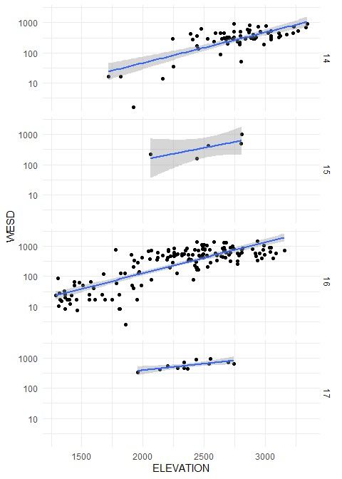
iii

                                        ABSTRACT

        Regionalized Models with Spatially Continuous Predictions at the Borders

                                             by

                           Jadon S. Wagstaff, Master of Science

                                Utah State University, 2021

Major Professor: Brennan Bean, Ph.D.
Department: Mathematics and Statistics

    Traditional spatial modeling approaches assume that data are second-order stationary,

which is rarely true over large geographical areas. A simple way to model nonstationary data

is to partition the space and build models for each region in the partition. This has the side

effect of creating discontinuities in the prediction surface at region borders. The regional

border smoothing approach described in this thesis ensures continuous predictions by using

a weighted average of predictions from regional models. The weights are based on the

shortest distance from the observation to each region boundary, with greater weight given

to observations that are within or near the boundaries of a region. The R package remap

is an implementation of the regional border smoothing method that builds a collection of

spatial models given a data set with spatial points, a set of polygon regions, and a modeling

approach to apply in each region. Special consideration is given to distance calculations that

make remap package scalable to large problems. Improvements in accuracy using the remap

package, as opposed to global spatial models, are illustrated using one national-level and

one state-level dataset. These accuracy improvements, coupled with their computational

feasibility, illustrate the efficacy of the remap approach to modeling nonstationary data.

                                                                                  (61 pages)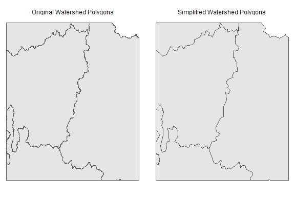
iv

                                  PUBLIC ABSTRACT

        Regionalized Models with Spatially Continuous Predictions at the Borders

                                    Jadon S. Wagstaff

    Creating maps of continuous variables involves estimating values between measurement

locations scattered throughout a geographic region. These maps often leverage observed

similarities between geographically close measurements, but may also make predictions

using other geographic information such as elevation. The relationship between the available

geographic information and the variable of interest can vary with location, especially when

mapping large areas like a continent. A simple way to account for the changing relationship

is to divide the space into different sub-regions and model the relationship at each region.

The naive implementation of this approach has the side effect of making sudden changes

in predictions at the borders of each region. This thesis describes a novel regional border

smoothing method that allows for the formation of a continuous map built with regional

models. The method is implemented and available to the public through the open source R

package remap. Improvements in model accuracy are demonstrated using a national scale

and a state scale dataset.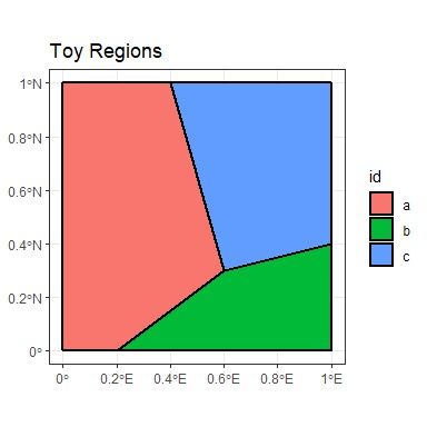
v

                                 ACKNOWLEDGMENTS

     Thank you Dr. Brennan Bean for your guidance, input, and support. Thanks also

to my committee members Dr. Jürgen Symanzik and Dr. Adele Cutler for your valuable

insight.

     This thesis was made possible in part by funding provided by the American Society of

Civil Engineers and the Structural Engineering Institute (award number 202827).

     Finally, a special thank you to Arianna Taylor, for your love and patience.

                                                                         Jadon S. Wagstaff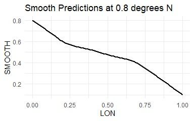
vi

                                                   CONTENTS

                                                                                                                       Page
ABSTRACT . . . . . . . . . . . . . . . . . . . . . . . . . . . . . . . . . . . . . . . . . . . . . . . . . . . . . . iii
PUBLIC ABSTRACT . . . . . . . . . . . . . . . . . . . . . . . . . . . . . . . . . . . . . . . . . . . . . . . iv
ACKNOWLEDGMENTS . . . . . . . . . . . . . . . . . . . . . . . . . . . . . . . . . . . . . . . . . . . .                       v
LIST OF TABLES . . . . . . . . . . . . . . . . . . . . . . . . . . . . . . . . . . . . . . . . . . . . . . . . . vii
LIST OF FIGURES . . . . . . . . . . . . . . . . . . . . . . . . . . . . . . . . . . . . . . . . . . . . . . . . viii
ACRONYMS . . . . . . . . . . . . . . . . . . . . . . . . . . . . . . . . . . . . . . . . . . . . . . . . . . . . .          ix
1   INTRODUCTION . . . . . . . . . . . . . . . . . . . . . . . . . . . . . . . . . . . . . . . . . . . . . . .                1
    1.1 Background . . . . . . . . . . . . . . . . . . . . . . . . . . . . . . . . . . . .                                    3
2   THE REGIONAL BORDER SMOOTHING APPROACH . . . . . . . . . . . . . . . . . .                                                6
    2.1 Smoothing at Borders . . . . . . . . . . . . . . . . . . . . . . . . . . . . . .                                      7
    2.2 A Note on Smoothing . . . . . . . . . . . . . . . . . . . . . . . . . . . . . .                                       8
3   REMAP . . . . . . . . . . . . . . . . . . . . . . . . . . . . . . . . . . . . . . . . . . . . . . . . . . . . . . 10
    3.1 Calculating Distances . . . . . . . . . . . . . . . . . . . . . . . . . . . . . .                             10
    3.2 Practical Implementation Considerations . . . . . . . . . . . . . . . . . . . .                               12
4   APPLICATIONS . . . . . . . . . . . . . . . . . . . . . . . . . . . . . .             ....    .....     ....    . . . . . 14
    4.1 National Snow Load Example . . . . . . . . . . . . .                             . . .   . . . .   . . .   . . .     14
        4.1.1 Building a Geospatial Snow Load Model . . .                                . . .   . . . .   . . .   . . .     14
        4.1.2 Building a Snow Load Prediction Grid . . . .                               . . .   . . . .   . . .   . . .     16
    4.2 Utah Snowpack Example . . . . . . . . . . . . . . .                              . . .   . . . .   . . .   . . .     18
5   CONCLUSIONS . . . . . . . . . . . . . . . . . . . . . . . . . . . . . . . . . . . . . . . . . . . . . . . . 21
APPENDICES . . . . . . . . . . . . . . . .       ....    .   ....    ....    ....    .   ....    ....    .....     . . . . . 27
  A remap Documentation . . .                    . . .   .   . . .   . . .   . . .   .   . . .   . . .   . . . .    . . .    28
     A.1   Package Manual . .                    . . .   .   . . .   . . .   . . .   .   . . .   . . .   . . . .    . . .    28
     A.2   Package Vignette . .                  . . .   .   . . .   . . .   . . .   .   . . .   . . .   . . . .    . . .    38
vii

                                       LIST OF TABLES

Table                                                                                             Page

   4.1   Ten fold cross-validation results from modeling the log of 50-year snow loads.
         Mean squared error (MSE) is multiplied by 102 for readability. Improvement
         is (national - regional) / national. . . . . . . . . . . . . . . . . . . . . . . . .       16

   4.2   Run times for redist to calculate geographic and projected distances from
         0.8 km grid points to 86 different eco-regions (polygons) in the conterminous
         US. Remedial steps are additive, i.e., each row in the table includes all pre-
         vious remedial steps. ∗ Approximate run time based on random sample of
         10,000 grid points. . . . . . . . . . . . . . . . . . . . . . . . . . . . . . . . .        18

   4.3   Ten fold cross-validation mean squared error from modeling log(WESD +
         1) for Utah snowpack. Mean squared error (MSE) is multiplied by 102 for
         readability. Improvement in parenthesise is calculated with (state - HUC) /
         state. . . . . . . . . . . . . . . . . . . . . . . . . . . . . . . . . . . . . . . . .     20
viii
LIST OF FIGURES
Figure Page
1.1 Before (top) and after (bottom) regional border smoothing is applied to re-
gional models where predictions are linear combinations of longitude and
latitude. The gray line shows predicted values along the 0.7°N transect. Left
region predicts lon − lat + 1, bottom region predicts lat − lon + 1.4, and right
region predicts lon − lat + 0.7. Smoothing zone is 30 km (≈ 0.27°). . . . . . 2
2.1 Example of a region’s buffer zone. A model is built for the red region using all
observations within a buffer zone (red dashed line). Red dots are observations
used to build the red region’s model. . . . . . . . . . . . . . . . . . . . . . . 7
2.2 Example of how predictions change as location approaches a region border.
In this example S = 50, the region on the “left” side of the border predicts a
constant value of one and the region on the “right” side of the border predicts
a constant value of two. . . . . . . . . . . . . . . . . . . . . . . . . . . . . . 8
2.3 Example of where predictions are not differentiable near non-convex regions.
The gray line shows predicted values along the 0.5°N transect. The bottom
region predicts a constant value of one and the top region predicts a constant
value of two. Smoothing zone is 40 km (≈ 0.36°). . . . . . . . . . . . . . . . 9
3.1 Example of what happens when predictions are made outside of any modeling
region. The gray line shows predicted values along the 0.6°N transect. The
dashed gray line shows predicted values along the 0.95°N transect. The left
region predicts a constant 0, the bottom region predicts a constant 2, and
the right region predicts a constant 4. Smoothing zone is 35 km (≈ 0.32°). . 13
4.1 Prediction map for 50-year loads from the regional GAM model built with
the remap package. Loads are shown on the log scale. Values are restricted
to be within the range of values observed in the load data. . . . . . . . . . . 16
4.2 Results of simplification of eco-regions. The highlighted region is an area
with some of the most severe gaps between polygons. Notice that the width
of the gaps are still much smaller than two times the smoothing parameter
(2 × 25 km). . . . . . . . . . . . . . . . . . . . . . . . . . . . . . . . . . . . . 17
4.3 HUC4 regions (lines) and HUC2 regions (shades) in Utah. . . . . . . . . . . 19ix
ACRONYMS
CRAN Comprehensive R Archive Network
EPA Environmental Protection Agency
GAM Generalized Additive Model
HUC Hydrologic Unit Code
MSE Mean Squared Error
NOAA National Oceanic and Atmospheric Administration
OLS Ordinary Least Squares
PRISM Parameter-elevation Regressions on Independent Slopes Model
SNOTEL Snowpack Telemetry
USGS United States Geological Survey
WESD Water Equivalent of Snow DepthCHAPTER 1
INTRODUCTION
Regression methods attempt to characterize the relationship between predictor vari-
ables and a response variable. When observations exhibit spatial autocorrelation, geographic
location can be leveraged to improve predictions of the response variable by considering ob-
served values of the response variable at nearby measurement locations. Typical spatial
statistical models assume that the covariance between two observations can be modeled as
a function of location difference, i.e., the relationship needs to be second-order stationary.
For sufficiently large distances, the stationarity assumption often fails.
The simplest way to effectively employ traditional spatial modeling approaches using
nonstationary data is to partition the global region into smaller sub-regions that are locally
stationary and create separate statistical models for each region. The naive implementation
of this approach leads to noncontinuous predictions at the borders of each region. Previous
attempts to smooth out discontinuities at region boundaries often involved taking weighted
averages of local regional model output where the weights of each local model prediction
or covariance structure are a function of the distance between a new observation and the
centers of each region (Fuentes, 2001; Fuentes & Smith, 2001; Gosoniu et al., 2009; Gosoniu
et al., 2006; Konomi et al., 2014). While the center based approach may be appropriate
for symmetrical regions, it may not be appropriate for oddly shaped or disjoint regions not
well approximated by their centers. In some cases, a region may not even contain its center.
The center based approach also fails to respect major geographic features that can cause
sharp changes in response variables over very short distances.
The regional border smoothing approach described in this thesis is a novel method
that uses a weighted average of predictions from local models, but gives weight to regional
models based on the nearest distance to the border of each region rather than distance to
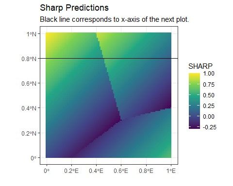
the center of each region. With this method, regions may be chosen that more naturally2
Fig. 1.1: Before (top) and after (bottom) regional border smoothing is applied to regional
models where predictions are linear combinations of longitude and latitude. The gray line
shows predicted values along the 0.7°N transect. Left region predicts lon − lat + 1, bottom
region predicts lat − lon + 1.4, and right region predicts lon − lat + 0.7. Smoothing zone is
30 km (≈ 0.27°).
reflect local climate and topography with smoothing only occurring near the borders of each
region. Figure 1.1 shows an example of the regional border smoothing approach applied to
three regions with different spatial models.
The R package remap is a General Public License implementation of this regional
border smoothing method that scales well to large problems (Wagstaff, 2021). Using remap,
regional border smoothing is applied to two different modeling problems. The first problem
is a national set of 50-year ground snow loads and the second problem is modeling April3
1st snow water content for Utah. Mapped values from both projects show improvement
in model accuracy using the regional border smoothing approach over global models for a
variety of spatial modeling approaches.
The figures and tables in this thesis are made using the R programming language (R
Core Team, 2020). Figures are created with the tidyverse (Wickham et al., 2019), gridExtra
(Auguie, 2017), cowplot (Wilke, 2020), and maps (Becker et al., 2018) packages. The sf
(Pebesma, 2018), nngeo (Dorman, 2020), and raster (Hijmans, 2020) packages are used to
manipulate spatial data. Kriging models are built with automap (Hiemstra et al., 2009)
and generalized additive models are built with mgcv (Wood, 2011).
1.1 Background
There are many proposed methods to model nonstationary data using locally stationary
models. Haas (1990a, 1990b) describes a moving window approach where only data within
a pre-specified bounding box are used to fit a local dependence structure and then make
predictions. This process is computationally intensive and may not result in continuous
predictions.
Fuentes (2001) and Fuentes and Smith (2001) propose a method for nonstationary
problems where a global covariance structure that changes continuously as a function of
location is used in a Gaussian process model. The data are first partitioned into locally
stationary regions. A global covariance structure is calculated by taking a weighted average
of regional covariance structures. Weights are based on the distance from the prediction
location to a point in each region, usually the center. Regions are either given a priori or
by using subgrids chosen using the Bayesian information criterion.
Applications of local partition modeling approaches include Kim et al. (2005), who
describe a method to deal with sudden changes in spatial covariance structure that occur
between layers of rock strata. The spatial domain is partitioned into independent regions
using Voronoi Tesselations (Green & Sibson, 1978), with each region fit using an independent
Gaussian model. The resulting global model has sharp changes at the borders of each
region, which was desirable in that context. Konomi et al. (2014) illustrate a decision4
tree based method for partitioning the spatial domain when modeling global Ozone levels.
Heaton et al. (2017) use a hierarchical clustering method to partition the spatial domain
for temperature data in Houston, TX. The hierarchical clustering method has the benefit of
creating a partition that more naturally follows changes in the covariance structure rather
than partitioning the space into symmetrical blocks or spheres.
Gosoniu et al. (2009) and Gosoniu et al. (2006) provide an additional application of
local partitioning models mapping malaria risk using a priori partitions of West Africa.
The 2006 study uses three large rectangular regions and the 2009 study uses agro-ecological
regions to partition the spatial domain. In these studies, spatial random effects are modeled
as a weighted sum of regional stationary effects based on the distance to region centroids.
The authors note problems with sudden changes at region borders as a result of using region
centroids for the weighted sum of effects.
Most of the methods discussed so far create a global covariance structure from local
covariance structures of Gaussian process models (Fuentes, 2001; Fuentes & Smith, 2001;
Heaton et al., 2017; Kim et al., 2005; Konomi et al., 2014). Each method has a different way
of smoothing regional transitions that are specifically tied to their methodology. Many of the
methods use a Bayesian framework that requires computationally expensive Markov chain
Monte Carlo simulations (Gosoniu et al., 2009; Gosoniu et al., 2006; Heaton et al., 2017;
Kim et al., 2005; Konomi et al., 2014). Many of the techniques are only applied to purely
spatial data rather than multivariate data (Heaton et al., 2017; Kim et al., 2005; Konomi
et al., 2014). This literature review highlights the lack of methodologies that allow for
smooth transitions between partitions and works for multiple modeling techniques. There
is also a general lack of software available to handle nonstationary data.
The regional border smoothing method described in this thesis can be thought of as
stitching together images to form a larger image with no sharp changes. The approach
is similar to those used to combine black and white images from microscopes into a larger
image (Thévenaz & Unser, 2007). Individual microscope images are aligned and the overlap-
ping regions are smoothed by taking a weighted average of the overlapping pixel brightness.5
The weights are based on the distance from the pixel to the outer edge of each image with
more weight being applied to pixels closer to the center of an image.
The process described in this thesis provides a simple way of combining regional model
predictions to form a continuous global prediction surface. The method can be applied to
problems that are not strictly spatial. For example, Osborne and Suárez-Seoane (2002)
show that building models for partitioned space can improve the accuracy of large scale
species distribution models. The regional border smoothing method works for any model
that produces a continuous prediction. A software implementation of the method described
in this thesis is available through the R package remap on the Comprehensive R Archive
Network (CRAN) (Wagstaff, 2021).
The remainder of this thesis proceeds with a description of the regional border smooth-
ing approach in Chapter 2. This is followed by Chapter 3 which describes the available
functions and tools in the remap package and Chapter 4 with two demonstrations of the
software on a state and national-level dataset. These demonstrations show the utility of the
remap package in producing smooth estimates when applied to large geographical problems
with irregularly shaped partitions.6
CHAPTER 2
THE REGIONAL BORDER SMOOTHING APPROACH
Regional border smoothing is the process of using regional models to make predictions
that are globally continuous. Regional border smoothing may be used on any spatially
X ) in conjunction with a modeling approach and a finite set of regions Rp
referenced data (X
where each Rpi ∈ Rp , i = 1 . . . m, is a closed set of points contained in the region of interest
R. The intention is that Rp is a set of non-overlapping polygons with shared borders and
m
S
Rp = R, but these are not necessary conditions. While Rp does not meet the strict
i=1
definition of a partition, Rp will be referred to as a partition throughout this thesis.
The border smoothing approach described in this thesis was originally designed for
regression-based models (such as kriging), but can be used with virtually any modeling
approach that predicts a continuous response. This technically includes classification tech-
niques that make continuous probability predictions prior to classifying based on a proba-
bility threshold. Presumably, the predictions from a chosen modeling approach will result
in continuous predictions as a function of location.
Modeling regions are defined by the borders of Rp . The data contained by a modeling
region Rpi are used to inform a distinct regression model (fpi (X
X )) for that region. In some
cases it may be desirable to include observations near each Rpi when building regional
regression models. In these cases, data within Rpi and possibly within a buffer zone around
each modeling region R∗pi are used to build each fpi (X
X ) (Figure 2.1). Using points within
a buffer zone that extends beyond the region boundaries avoids edge extrapolation when
using a regional model for interpolation in the smoothing zones of neighboring regions. See
Section 2.1 for additional details.
Simply making predictions within each Rpi using each corresponding fpi (X
X ) results
in noncontinuous predictions at region boundaries. Regional border smoothing results in
continuous predictions for the entire space by taking a weighted average of the predictions7
Fig. 2.1: Example of a region’s buffer zone. A model is built for the red region using all
observations within a buffer zone (red dashed line). Red dots are observations used to build
the red region’s model.
X ). The smoothed global prediction surface is continuous, but not
provided by each fpi (X
necessarily differentiable (see Section 2.2).
2.1 Smoothing at Borders
x∗ ), fp2 (x
Let ŷ1 , ŷ2 , ..., ŷm represent predictions from regional models fp1 (x x∗ ), ..., fpm (x
x∗ )
for location of interest x ∗ where x ∗ represents both spatial and non-spatial information. A
final prediction ŷ 0 is calculated by the weighted average of each ŷ, i.e.,
w(d1 |S)ŷ1 + w(d2 |S)ŷ2 + ... + w(dm |S)ŷm
ŷ 0 = . (2.1)
w(d1 |S) + w(d2 |S) + ... + w(dm |S)
The weights are calculated based on the smallest great-circle distances (d1 , d2 , ..., dm )8
Fig. 2.2: Example of how predictions change as location approaches a region border. In
this example S = 50, the region on the “left” side of the border predicts a constant value
of one and the region on the “right” side of the border predicts a constant value of two.
between the location of x ∗ and the boundaries of Rp1 , Rp2 , ..., Rpm . If x ∗ is located within
a region, the distance between x∗ and that region is 0. The weight w(di |S) given to ŷi is
non-zero when di is within some threshold S, i.e.,
2
S−di
S di ≤ S
w(di |S) = (2.2)
0
di > S.
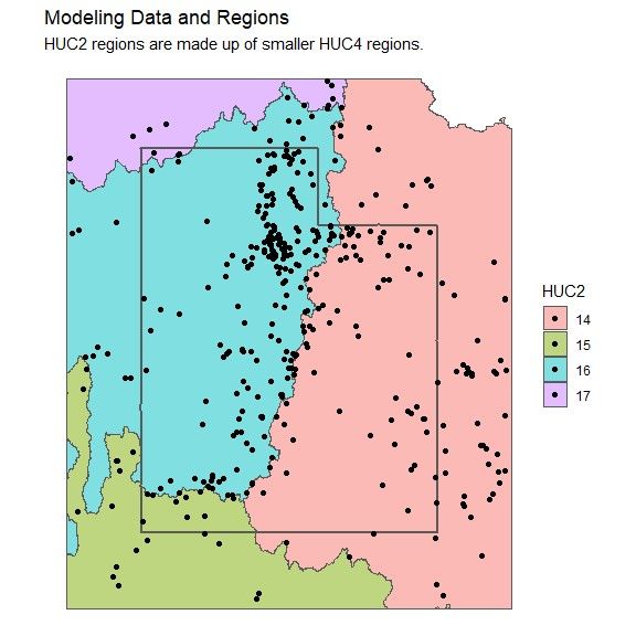
Consider now the special case when a prediction is made in region j and di6=j > S,
then w(di6=j |S) = 0 and Equation 2.1 reduces to ŷ 0 = ŷj . As prediction locations in region
ŷj +((S−dk )/S)2 ŷk
j approach Rpk , then the weight of ŷk increases gradually and ŷ 0 = 1+((S−dk )/S)2
. At
ŷj +ŷk
the border of regions j and k, ŷ = 2 . Finally, as prediction locations progress into Rpk ,
((S−dj )/S)2 ŷj +ŷk
weights for yij decrease gradually to zero and ŷ 0 = ((S−dj )/S)2 +1
. Figure 2.2 shows a
simple example of how predictions change across region borders. All locations within S of
a region are referred to as the smoothing zone for that region.
2.2 A Note on Smoothing
The “smoothing” described throughout this thesis refers to smoothing in the colloquial
sense. A continuous prediction surface is created with a steady transition between regions.
The prediction surface is not always differentiably smooth. If a region is not convex, the
rate of change in the distance to a region can shift suddenly at locations that are equidistant9
Fig. 2.3: Example of where predictions are not differentiable near non-convex regions. The
gray line shows predicted values along the 0.5°N transect. The bottom region predicts a
constant value of one and the top region predicts a constant value of two. Smoothing zone
is 40 km (≈ 0.36°).
to different parts of the region. Figure 2.3 shows an example of a prediction surface near a
non-convex region where the prediction surface is not differentiably smooth.
Since each region is a closed set of points, di is continuous. It therefore follows that
the weight function w(di |S) described in Equation 2.2 is continuous as limx→0+ w(x|S) =
w(0|S) = 1 and limx→S − w(x|S) = w(S|S) = 0 for x ∈ [0, ∞) and S > 0. Since Equation
2.1 includes the multiplication and addition of continuous functions, it is guaranteed to
have max (w(di |S)) > 0 as long as x ∗s is within S units of any Rp and it follows that ŷ 0 is
also continuous. Given continuous predictions as a function of location for each region, the
regional border smoothing method is guaranteed to be continuous for any location within
the smoothing zone of at least one region. Once all di > S, then the denominator of y 0 is
equal to zero, which means y 0 is no longer well-defined. As long as all of the data X are
located within Rp , any prediction location outside of Rp is spatial extrapolation that is
generally discouraged.10
CHAPTER 3
REMAP
The R package remap (Wagstaff, 2021) is an implementation of the regional border
smoothing approach to spatial modeling. The function remap creates a set of regionalized
models given:
• A set of spatially referenced observations (projected or geographic).
• A set of spatially referenced polygons defining the regions.
• A desired buffer zone distance.
• A modeling function to apply to observations in each region.
Predictions can be made on new observations given a regionalized model and the smooth-
ing parameter smooth used for weighted averages in smoothing zones (variable S in Equa-
tion 2.2). Detailed descriptions of function parameters can be found in the package doc-
umentation which is also available in Appendix A.1. Some working examples using the
remap package are provided via the vignette which accompanies the package and avail-
able in Appendix A.2. The development version of the code for remap can be found at
https://github.com/jadonwagstaff/remap.
3.1 Calculating Distances
The weights for regional predictions require the distances from all observations to
the boundary of each region. The modeling process of the remap function also requires
the distances from all observations to the boundary of each region to assign the correct
observations to each regional model. The process of fine-tuning a model can result in
recalculating these distances many times. To avoid recalculating distances, the function
redist is included in the remap package to pre-compute the distances from a given set of11
observations to a given set of regions. These pre-computed distances can be supplied as a
parameter to the remap function to reduce computational time while fine-tuning models.
Calculating distances in the remap package takes advantage of tools already available
for spatial analysis in the R package sf (Pebesma, 2018). The function sf::st distance is
used to find either Euclidean or great-circle distances depending on the spatial projection
of the locations and regions. The sf::st distance function uses the S2 library (Google,
2020) when calculating great-circle distances. The S2 library is designed specifically to
efficiently compute distances between nearby objects given large sets of geographic data.
Regardless, calculating distances can still take a lot of computational time if the regions are
complex and/or there are a lot of observations.
The naı̈ve approach to regional border smoothing is to find all distances between each
location and each region. This approach may be necessary during the modeling process if
any region does not contain a required minimum number of observations (see Section 3.2).
If predictions are being made using new observations, then distances do not need to be
calculated between every observation and every region.
Because the weight for predictions in different regions is zero when the distance to
those regions is greater than the smoothing parameter (Equation 2.2), distances do not
need to be calculated between every region and every prediction location. To determine
which observations require distance calculations, an approximate polygon is constructed
that encompasses the original region plus the smoothing zone around the region. The func-
tion sf::st within is used to determine which observations are within the new polygon
and equivalently, which observations are within the smoothing zone of the original region.
Observations in the approximate polygon become candidates for precise distance calcula-
tions.
An approximate polygon that contains a region and the region’s smoothing zone is
created using the sf::st buffer function. For geographic coordinates, sf::st buffer
requires a buffer value in degrees. Since the great-circle distance between a unit degree
of longitude changes with latitude, Equation 3.1 is used to find c: the shortest distance12
(measured in kilometers) required to move one degree longitude at the observation in the
dataset that is nearest to a geographical pole. λ represents the vector of latitudes for each
observation and 6350 km is the radius of the earth at a pole (rounded down). A sufficient
buffer value in degrees for sf::st buffer is calculated by dividing the smoothing zone
length in km by c. The resulting buffered polygon contains all of the observations within
the smoothing zone of the original polygon.
π ∗ 6350 π ∗ max(|λ
λ|)
c= ∗ cos (3.1)
180 180
Assuming each region contains a sufficient number of observations to fit each regional
model, the same process used for reducing the number of distance calculations for model
training can be used to reduce the number of distance calculations required for model
predictions. (See Section 3.2 for a description of what happens when the observations in a
region fall below a minimum sample size threshold.) The function redist is able to restrict
distance calculations to only observations within a certain buffer or smoothing zone of each
region using the max dist parameter. This eliminates the need to calculate distances to
points with a known weight of zero when smoothing.
3.2 Practical Implementation Considerations
Reliable regression results depend upon sufficient sample sizes, which differ based on
the variability of the response and dimensionality of the inputs. A strict (and obvious)
minimum sample size for the remap function is one observation per region, though this
threshold will rarely, if ever, ensure reasonable results. An additional parameter min n is
included in the remap function to specify a minimum number of observations used to build
each model. If a region and the buffer around that region do not contain the minimum
number of observations specified, the min n observations closest to the boundaries of the
region are used to train that region’s model.
The remap package has the ability to make predictions outside of all modeling regions.
If the prediction location is within the smoothing zone of a region, then Equation 2.1 is still13
Fig. 3.1: Example of what happens when predictions are made outside of any modeling
region. The gray line shows predicted values along the 0.6°N transect. The dashed gray line
shows predicted values along the 0.95°N transect. The left region predicts a constant 0, the
bottom region predicts a constant 2, and the right region predicts a constant 4. Smoothing
zone is 35 km (≈ 0.32°).
used and the nearest region will have the most weight. If the prediction location is outside
the smoothing zone of all regions, then the model from the closest region is used to make
a prediction. This may result in non-continuous transitions in predictions when the closest
region changes across geographic space, but this is only possible at locations outside of the
smoothing zone of all regions. As a general rule, extrapolation of predictions to locations
beyond those represented in the input data is not recommended. See Figure 3.1 for a visual
depiction of how predictions behave outside of all modeling regions.
The ability to predict outside of all regions means that the remap package can make
smooth predictions across small gaps at polygon borders, provided the gaps are no larger
than two times the smoothing zone distance. This encourages the use of rgeos::gSimplify
(Bivand & Rundel, 2020) or sf::st simplify (Pebesma, 2018) to simplify complex poly-
gons and ease the computational burden associated with distance calculations, even if those
simplifications slightly compromise the topology of the original geometry.14
CHAPTER 4
APPLICATIONS
4.1 National Snow Load Example
Snow loads are obtained from weather stations throughout the United States in the
National Oceanic and Atmospheric Administration’s (NOAA) Global Historical Climatology
Network (Menne et al., 2012). Snow loads are either measured directly, or estimated from
measured snow depth using a depth to load conversion model. Engineers have historically
used estimates of 50-year ground snow loads when designing structures. The 50-year snow
load is traditionally obtained by fitting a probability distribution to yearly maximum snow
load measurements and extracting the 98th percentile. A recent effort by the American
Society of Civil Engineers has resulted in a new set of 50-year ground snow loads at 7964
measurement locations. The 50-year loads are calculated in a similar manner to Bean
et al. (2018), except yearly maximum snow loads are fit to the generalized extreme value
distribution instead of the log-normal distribution.
4.1.1 Building a Geospatial Snow Load Model
Building design requirements call for continuous maps that estimate design loads be-
tween measurement locations. This has historically been accomplished using various map-
ping techniques (Bean et al., 2019; Liel et al., 2017; Tobiasson et al., 2002). The problem is
that the relationship between predictor variables and snow load can change drastically on a
continental scale. For example, the typical loads at 5000 feet elevation in the Rocky Moun-
tains of Colorado are much lower than typical loads at 5000 feet in the Cascade Mountains
of Washington State. Commonly used geospatial models for mapping are not well suited
for the nonstationary nature of this problem.
Geographic regions defined by the US Environmental Protection Agency (EPA) define15
regions with similar ecology and climate called eco-regions (Commission for Environmen-
tal Cooperation, 1997). The eco-regions provide a natural partition of the conterminous
United States and give no regard to political boundaries. Snow load can be modeled using
observations within each eco-region where the relationship between predictor variables and
the response is more consistent on a local level. The remap package facilitates modeling in
separate eco-regions and creates a smooth model on the national scale.
Snow loads are typically assumed to share a log-linear relationship with elevation. This
relationship is modeled directly using ordinary least squares (OLS). A generalized additive
model (GAM) built with the mgcv R package (Wood, 2011) characterizes the log of 50-
year loads as a function of elevation and a spatial smoother called splines on the sphere
(Wood, 2003). Universal kriging interpolates values using a Gaussian process model after
accounting for the log-linear trend in elevation with the automap R package (Hiemstra
et al., 2009). Parameter-elevation regressions on independent slopes model (PRISM) is a
modeling method that uses a form of weighted linear regression to model loads as a function
of elevation (Daly et al., 2002; Daly et al., 2008). The adaptation of PRISM to estimate
snow loads in this thesis is described in Bean et al. (2017).
Some of the methods for mapping snow loads are compared in Table 4.1 using national
scale models and models built with the remap package on EPA Level III Eco-Regions
(Commission for Environmental Cooperation, 1997). There are 86 eco-regions that fall
within the conterminous United States, so 86 separate models are built using the remap
function with a buffer zone of 50 km and a min n of 150 observations. The regional models
are smoothed to a single continuous model using a smooth parameter of 25 km.
The results in Table 4.1 show that the remap package framework improves the cross
validated accuracy of every spatial modeling method. This demonstrates that the remap
package has the ability to generally improve modeling results, as improvements are not
isolated to a single spatial modeling case. Even though the regional models are made up of
86 different regional models, the estimated 50-year loads are smooth across the prediction
surface (see Figure 4.1).16
MSE ×102
Model Improvement
National Regional
GAM 8.2 5.5 33%
Kriging 7.2 5.9 18%
PRISM 21.0 7.9 62%
OLS 89.3 17.8 80%
Table 4.1: Ten fold cross-validation results from modeling the log of 50-year snow loads.
Mean squared error (MSE) is multiplied by 102 for readability. Improvement is (national -
regional) / national.
Fig. 4.1: Prediction map for 50-year loads from the regional GAM model built with the
remap package. Loads are shown on the log scale. Values are restricted to be within the
range of values observed in the load data.
4.1.2 Building a Snow Load Prediction Grid
National snow load maps require a sufficiently fine resolution to be feasibly used to
design buildings in topographically complex areas. To accomplish this, snow load maps are
created that match the resolution of PRISM climate output (PRISM Climate Group, 2020),
which maps at a 0.8 km resolution for the conterminous United States. This means that
predicted snow loads are calculated at 12,113,556 locations using a model created by the
remap package with 86 different regions. Elevation values for the grid are obtained from
the United States Geological Survey (United States Geological Survey, 2020b).
Since the remap package uses the distances between prediction locations and regions to
make a smooth model, calculating these distances is a potential bottleneck in the prediction17
Fig. 4.2: Results of simplification of eco-regions. The highlighted region is an area with
some of the most severe gaps between polygons. Notice that the width of the gaps are still
much smaller than two times the smoothing parameter (2 × 25 km).
process. Also, since the prediction area is so large, geographic coordinates rather than
projected coordinates must be used to find distances. This further increases the bottleneck
since great circle distances require more resources to compute than Euclidean distances.
Simply calculating all distances would have taken over a year to run on a typical desktop
computer, as illustrated in Table 4.2. The test computer used for Table 4.2 has 16 GB of
RAM and an Intel Core I5-4590 CPU which runs at 3.3 GHz.
The first step to reduce the run time for distance calculations is to simplify the polygons
as discussed in Section 3.2. Using a tolerance of 0.1◦ with the function sf::st simplify, the18
Run time in hours
Remedial steps
Geographic Projected
None 15000.0 ∗ 200.0∗
Simplify polygons 44.0 ∗ 1.4
+ set max dist to 25 km 1.8 1.0
+ run in parallel on 4 cores 1.3 1.0
Table 4.2: Run times for redist to calculate geographic and projected distances from 0.8
km grid points to 86 different eco-regions (polygons) in the conterminous US. Remedial steps
are additive, i.e., each row in the table includes all previous remedial steps. ∗ Approximate
run time based on random sample of 10,000 grid points.
size of the polygons are reduced from 21 MB to 0.2 MB. The results of polygon simplification
are visualized in Figure 4.2. When making predictions, the smooth parameter is set to 25
km; therefore, the max dist parameter of redist can be set to 25 km to further reduce
run time. Finally, combining the previous steps and running in parallel on four cores, the
relevant distances are calculated for all points using great circle distance in about 1.3 hours
(Table 4.2). This tremendous computational speed-up is made possible by the ability of the
remap package to smoothly fill in the gaps that occur in aggressively simplified polygons.
4.2 Utah Snowpack Example
The state of Utah assesses snow water content or snowpack every April 1st to plan
for yearly water resource availability. These measurements are much more variable than
the 50-year snow loads since the values are based on a single measurement at each location
instead of the 98th percentile of a distribution fit to annual maximum values at each location.
This example uses direct measurements of the water content made via Snowpack Telemetry
(SNOTEL) stations included in NOAA’s Global Historical Climatology Network (Menne et
al., 2012). In addition to SNOTEL station data, Snow Course data collected by the National
Water and Climate Center are also included in the dataset (Natural Resources Conservation
Service, 2017). SNOTEL and Snow Course data measure the water equivalent of snow depth
(WESD) and are located in the mountainous areas of Utah above 1777 m elevation. This
negates the need to estimate water content from snow depth, which is typically the case
when measuring snow at non-mountainous locations in the state.19
Fig. 4.3: HUC4 regions (lines) and HUC2 regions (shades) in Utah.
SNOTEL stations and Snow Course data within 100 km of the border of Utah are
included in the dataset. There are 3511 April 1st WESD observations available for modeling
which range from 0 to 1746 mm of water. The observations have 178 unique locations and
span 30 years (1986-2015). Each year is modeled separately with no regard for any temporal
correlations and each year has at least 97 observations.
Models for GAM, kriging, PRISM, and OLS are created using the same model structure
as the national snow load example, but a different response variable. Since there are 142 zero
values for WESD within the data, the log of (WESD + 1) is used as the response variable
for the April 1st snowpack. Predictions are also constrained to be between [1, max(WESD)]
to avoid excessive extrapolation. The regions used for regional modeling are watershed
boundaries defined by the USGS (United States Geological Survey, 2020a). Watersheds
are defined by a hierarchy of hydrologic unit codes (HUC) with a two-digit designation for
continental scale watersheds (HUC2) and a four-digit designation that partitions each HUC2
region (HUC4). There are four HUC2 regions and 12 HUC4 regions within the boundaries
of the state of Utah (see Figure 4.3). A buffer zone of 20 km, a smoothing parameter of 10
km, and a min n of 30 observations are used when modeling both HUC2 and HUC4 regions
with the remap function.20
MSE ×102
Model
State HUC2 HUC4
GAM 85 74(13%) 79 (7%)
Kriging 92 90 (2%) 85 (8%)
PRISM 93 86 (7%) 81(13%)
OLS 140 109(22%) 89(36%)
Table 4.3: Ten fold cross-validation mean squared error from modeling log(WESD + 1) for
Utah snowpack. Mean squared error (MSE) is multiplied by 102 for readability. Improve-
ment in parenthesise is calculated with (state - HUC) / state.
Table 4.3 shows that the gains in accuracy are more modest in this application than in
the national example shown previously. This is expected as the partitions are on the state
level instead of the national level. Nevertheless, the consistent improvement in accuracy at
various scales using different polygons and input data highlight the general ability of the
remap package to improve predictive accuracy without sacrificing continuity.21
CHAPTER 5
CONCLUSIONS
Partitioning a space for geospatial modeling is a practical approach for handling non-
stationary data; however, smooth transitions in mapped values are a desirable constraint
of many data products, such as the design snow load requirements set forth by the Amer-
ican Society of Engineers. The remap R package provides a ready-to-use framework for
regional models with smooth transitions at region borders that overcomes the computa-
tional difficulties of naive implementations. This package is available on the Comprehensive
R Archive Network (see https://cran.r-project.org/web/packages/remap/index.html) with
the most current version available at https://github.com/jadonwagstaff/remap.
The remap package creates continuous prediction surfaces by weighting regional pre-
dictions based on the proximity to region borders. Smoothing at region borders makes
the package particularly equipped to handle irregularly shaped regions not well represented
by their geographic centers. Because the remap package has the ability to smooth over
small gaps formed when simplifying polygons, computation times can be drastically re-
duced without sacrificing the continuity of the predictions. Methods that automatically
subset the number of required distance calculations further reduce computational times.
This thesis has demonstrated accuracy improvements using the remap package on two sep-
arate datasets with two sets of polygon inputs. These examples highlight the feasibility of
applying the remap framework to spatial regression modeling problems.22
Bibliography
Auguie, B. (2017). gridExtra: Miscellaneous functions for ”grid” graphics [R package ver-
sion 2.3]. https://CRAN.R-project.org/package=gridExtra
Bean, B., Maguire, M., & Sun, Y. (2017). Predicting Utah ground snow loads with PRISM.
Journal of Structural Engineering, 143 (9), 04017126. https : / / doi . org / 10 . 1061 /
(ASCE)ST.1943-541X.0001870
Bean, B., Maguire, M., & Sun, Y. (2018). The Utah snow load study (tech. rep. No. 3589).
Utah State University, Department of Civil and Environmental Engineering. https:
//digitalcommons.usu.edu/cee facpub/3589
Bean, B., Maguire, M., & Sun, Y. (2019). Comparing design ground snow load prediction
in Utah and Idaho. Journal of Cold Regions Engineering, 33 (3), 04019010. https:
//doi.org/10.1061/(ASCE)CR.1943-5495.0000190
Becker, R. A., Wilks, A. R., Brownrigg, R., Minka, T. P., & Deckmyn, A. (2018). maps:
Draw geographical maps [R package version 3.3.0]. https://CRAN.R- project.org/
package=maps
Bivand, R., & Rundel, C. (2020). rgeos: Interface to geometry engine - open source (’GEOS’)
[R package version 0.5-5]. https://CRAN.R-project.org/package=rgeos
Commission for Environmental Cooperation. (1997). Ecological regions of North America:
Toward a common perspective (tech. rep.) [Accessed: 2020-04-09]. Commission for
Environmental Cooperation. http : / / www3 . cec . org / islandora / en / item / 1701 -
ecological-regions-north-america-toward-common-perspective
Daly, C., Gibson, W. P., Taylor, G. H., Johnson, G. L., & Pasteris, P. (2002). A knowledge-
based approach to the statistical mapping of climate. Climate Research, 22 (2), 99–
113. https://doi.org/10.3354/cr022099
Daly, C., Halbleib, M., Smith, J. I., Gibson, W. P., Doggett, M. K., Taylor, G. H., Curtis,
J., & Pasteris, P. P. (2008). Physiographically sensitive mapping of climatological23
temperature and precipitation across the conterminous United States. International
Journal of Climatology, 28 (15), 2031–2064. https://doi.org/10.1002/joc.1688
Dorman, M. (2020). nngeo: K-nearest neighbor join for spatial data [R package version
0.4.0]. https://CRAN.R-project.org/package=nngeo
Fuentes, M. (2001). A high frequency kriging approach for non-stationary environmental
processes. Environmetrics, 12 (5), 469–483. https://doi.org/10.1002/env.473
Fuentes, M., & Smith, R. L. (2001). A new class of nonstationary spatial models (tech. rep.).
North Carolina State University. https://repository.lib.ncsu.edu/bitstream/handle/
1840.4/213/nonstat.pdf?sequence=1
Google. (2020). S2 [Source code]. https://github.com/google/s2geometry
Gosoniu, L., Vounatsou, P., Sogoba, N., Maire, N., & Smith, T. (2009). Mapping malaria
risk in West Africa using a Bayesian nonparametric non-stationary model. Compu-
tational Statistics & Data Analysis, 53 (9), 3358–3371. https://doi.org/10.1016/j.
csda.2009.02.022
Gosoniu, L., Vounatsou, P., Sogoba, N., & Smith, T. (2006). Bayesian modelling of geosta-
tistical malaria risk data. Geospatial Health, 1, 127–39. https://doi.org/10.4081/gh.
2006.287
Green, P. J., & Sibson, R. (1978). Computing Dirichlet tessellations in the plane. The
Computer Journal, 21 (2), 168–173. https://doi.org/10.1093/comjnl/21.2.168
Haas, T. C. (1990a). Kriging and automated variogram modeling within a moving window.
Atmospheric Environment. Part A. General Topics, 24 (7), 1759–1769. https://doi.
org/10.1016/0960-1686(90)90508-K
Haas, T. C. (1990b). Lognormal and moving window methods of estimating acid deposition.
Journal of the American Statistical Association, 85 (412), 950–963. https://doi.org/
10.1080/01621459.1990.10474966
Heaton, M. J., Christensen, W. F., & Terres, M. A. (2017). Nonstationary Gaussian process
models using spatial hierarchical clustering from finite differences. Technometrics,
59 (1), 93–101. https://doi.org/10.1080/00401706.2015.110276324
Hiemstra, P., Pebesma, E., Twenhöfel, C., & Heuvelink, G. (2009). Real-time automatic
interpolation of ambient gamma dose rates from the Dutch radioactivity monitoring
network. Computers & Geosciences, 35 (8), 1711–1721. https://doi.org/10.1016/j.
cageo.2008.10.011
Hijmans, R. J. (2020). raster: Geographic data analysis and modeling [R package version
3.4-5]. https://CRAN.R-project.org/package=raster
Kim, H.-M., Mallick, B. K., & Holmes, C. C. (2005). Analyzing nonstationary spatial data
using piecewise Gaussian processes. Journal of the American Statistical Association,
100 (470), 653–668. https://doi.org/10.1198/016214504000002014
Konomi, B. A., Sang, H., & Mallick, B. K. (2014). Adaptive Bayesian nonstationary model-
ing for large spatial datasets using covariance approximations. Journal of Computa-
tional and Graphical Statistics, 23 (3), 802–829. https://doi.org/10.1080/10618600.
2013.812872
Liel, A. B., DeBock, D. J., Harris, J. R., Ellingwood, B. R., & Torrents, J. M. (2017).
Reliability-based design snow loads. II: Reliability assessment and mapping proce-
dures. Journal of Structural Engineering, 143 (7), 04017047. https://doi.org/10.
1061/(ASCE)ST.1943-541X.0001732
Menne, M., Durre, I., Korzeniewski, B., Vose, R., Gleason, B., & Houston, T. (2012). Global
historical climatology network - daily, version 3.26 [Accessed: 2020-06-04]. https :
//doi.org/10.7289/V5D21VHZ
Natural Resources Conservation Service. (2017). Snow course stations [Accessed: 2020-04-
03]. https://wcc.sc.egov.usda.gov/reportGenerato
Osborne, P. E., & Suárez-Seoane, S. (2002). Should data be partitioned spatially be-
fore building large-scale distribution models? Ecological Modelling, 157 (2), 249–259.
https://doi.org/10.1016/S0304-3800(02)00198-9
Pebesma, E. (2018). Simple features for R: Standardized support for spatial vector data.
The R Journal, 10 (1), 439–446. https://doi.org/10.32614/RJ-2018-00925
PRISM Climate Group. (2020). 30-year normals. Northwest Alliance for Computational
ScienceEngineering. https://prism.oregonstate.edu/normals/
R Core Team. (2020). R: A language and environment for statistical computing. R Founda-
tion for Statistical Computing. Vienna, Austria. https://www.R-project.org/
Thévenaz, P., & Unser, M. (2007). User-friendly semiautomated assembly of accurate image
mosaics in microscopy. Microscopy Research and Technique, 70 (2), 135–146. https:
//doi.org/10.1002/jemt.20393
Tobiasson, W., Buska, J., Greatorex, A., Tirey, J., & Fisher, J. (2002). Ground snow loads
for New Hampshire (tech. rep.). Cold Regions Research and Engineering Laboratory.
Hanover, New Hampshire. https://www.senh.org/wp- content/uploads/2010/12/
tr02-6.pdf
United States Geological Survey. (2020a). National hydrography dataset [Accessed: 2020-
10-16]. https://www.usgs.gov/core- science- systems/ngp/national- hydrography/
access-national-hydrography-products
United States Geological Survey. (2020b). The national map [Accessed: 2020-04-01]. https:
//www.usgs.gov/core-science-systems/national-geospatial-program/national-map
Wagstaff, J. (2021). remap: Regional spatial modeling with continuous borders [R package
version 0.2.0]. https://github.com/jadonwagstaff/remap
Wickham, H., Averick, M., Bryan, J., Chang, W., McGowan, L. D., François, R., Grolemund,
G., Hayes, A., Henry, L., Hester, J., Kuhn, M., Pedersen, T. L., Miller, E., Bache,
S. M., Müller, K., Ooms, J., Robinson, D., Seidel, D. P., Spinu, V., . . . Yutani, H.
(2019). Welcome to the tidyverse. Journal of Open Source Software, 4 (43), 1686.
https://doi.org/10.21105/joss.01686
Wilke, C. O. (2020). cowplot: Streamlined plot theme and plot annotations for ggplot2 [R
package version 1.1.1]. https://CRAN.R-project.org/package=cowplot
Wood, S. N. (2011). Fast stable restricted maximum likelihood and marginal likelihood esti-
mation of semiparametric generalized linear models. Journal of the Royal Statistical
Society (B), 73 (1), 3–36. https://doi.org/10.1111/j.1467-9868.2010.00749.x26
Wood, S. N. (2003). Thin plate regression splines. Journal of the Royal Statistical Society:
Series B (Statistical Methodology), 65 (1), 95–114. https://doi.org/10.1111/1467-
9868.0037427 APPENDICES
28

                                       APPENDIX A

                                   remap Documentation

A.1     Package Manual

      The package manual describes all of the functions in remap, describes their parameters,

and describes the output objects. The manual is printed as it appears at https://cran.

r-project.org/web/packages/remap/remap.pdf.
29
Package ‘remap’
January 14, 2021
Type Package
Title Regional Spatial Modeling with Continuous Borders
Version 0.2.0
Description Automatically creates separate regression models for different spatial regions.
The prediction surface is smoothed using a novel method developed by the package creator.
If regional models are continuous, the resulting prediction surface is continuous across
the spatial dimensions, even at region borders.
License GPL-3
URL https://github.com/jadonwagstaff/remap
BugReports https://github.com/jadonwagstaff/remap/issues
Encoding UTF-8
LazyData true
Imports graphics (>= 3.6.0), parallel (>= 3.6.0), sf (>= 0.9.6), stats
(>= 3.6.0), units (>= 0.6.7), utils (>= 3.6.0)
RoxygenNote 7.1.1
Suggests dplyr (>= 1.0.2), ggplot2 (>= 3.3.2), knitr (>= 1.30), lwgeom
(>= 0.2.5), magrittr (>= 2.0.1), maps (>= 3.3.0), mgcv (>=
1.8.33), rmarkdown (>= 2.5), tibble (>= 3.0.4)
VignetteBuilder knitr
Depends R (>= 3.6.0)
NeedsCompilation no
Author Jadon Wagstaff [aut, cre]
Maintainer Jadon Wagstaff
Repository CRAN
Date/Publication 2021-01-14 10:30:02 UTC
130
2 predict.remap
R topics documented:
plot.remap . . . . . . . . . . . . . . . . . . . . . . . . . . . . . . . . . . . . . . . . . . 2
predict.remap . . . . . . . . . . . . . . . . . . . . . . . . . . . . . . . . . . . . . . . . 2
print.remap . . . . . . . . . . . . . . . . . . . . . . . . . . . . . . . . . . . . . . . . . 3
redist . . . . . . . . . . . . . . . . . . . . . . . . . . . . . . . . . . . . . . . . . . . . 4
remap . . . . . . . . . . . . . . . . . . . . . . . . . . . . . . . . . . . . . . . . . . . . 5
utsnow . . . . . . . . . . . . . . . . . . . . . . . . . . . . . . . . . . . . . . . . . . . . 7
utws . . . . . . . . . . . . . . . . . . . . . . . . . . . . . . . . . . . . . . . . . . . . . 8
Index 9
plot.remap Plot method for remap object.
Description
Plots the regions used for modeling.
Usage
## S3 method for class 'remap'
plot(x, ...)
Arguments
x S3 object output from remap.
... Arguments to pass to regions plot.
Value
A list that plots a map of the regions used for modeling.
predict.remap Make predictions given a set of data and smooths predictions at region
borders. If an observation is outside of all regions and smoothing
distances, the closest region will be used to predict.
Description
Make predictions given a set of data and smooths predictions at region borders. If an observation is
outside of all regions and smoothing distances, the closest region will be used to predict.
Usage
## S3 method for class 'remap'
predict(object, data, smooth, distances, cores = 1, progress = FALSE, ...)31
print.remap 3
Arguments
object S3 object output from remap.
data An sf dataframe with point geometry.
smooth The distance in km within a region where a smooth transition to the next region
starts. If smooth = 0, no smoothing occurs between regions unless an observa-
tion falls on the border of two or more polygons. (Can be a named vector with
different values for each unique object$region_id’ in ’ object$region’.)
distances An optional matrix of distances between ’data’ and ’object$regions’ generated
by redist() function (calculated internally if not provided).
cores Number of cores for parallel computing. ’cores’ above default of 1 will require
more memory.
progress If true, a text progress bar is printed to the console. (Progress bar only appears
if ’cores’ = 1.)
... Arguments to pass to individual model prediction functions.
Value
Predictions in the form of a numeric vector.
See Also
remap building a regional model.
print.remap Print method for remap object.
Description
Print method for remap object.
Usage
## S3 method for class 'remap'
print(x, ...)
Arguments
x S3 object output from remap.
... Extra arguments.
Value
No return value, a description of the remap object is printed in the console.You can also read