Enhanced Field-Based Detection of Potato Blight in Complex Backgrounds Using Deep Learning

AAAS
Plant Phenomics
Volume 2021, Article ID 9835724, 13 pages
https://doi.org/10.34133/2021/9835724

Research Article
Enhanced Field-Based Detection of Potato Blight in Complex
Backgrounds Using Deep Learning

 Joe Johnson ,1 Geetanjali Sharma,1 Srikant Srinivasan ,1 Shyam Kumar Masakapalli,2
 Sanjeev Sharma,3 Jagdev Sharma,3 and Vijay Kumar Dua3
 1
 School of Computing & Electrical Engineering, Indian Institute of Technology Mandi, Kamand, H.P., India
 2
 BioX Center, School of Basic Sciences, Indian Institute of Technology Mandi, Kamand, H.P., India
 3
 ICAR-Central Potato Research Institute, H.P., Shimla, India

 Correspondence should be addressed to Srikant Srinivasan; srikant_srinivasan@iitmandi.ac.in

 Received 1 August 2020; Accepted 26 March 2021; Published 16 May 2021

 Copyright © 2021 Joe Johnson et al. Exclusive Licensee Nanjing Agricultural University. Distributed under a Creative Commons
 Attribution License (CC BY 4.0).

 Rapid and automated identification of blight disease in potato will help farmers to apply timely remedies to protect their produce.
 Manual detection of blight disease can be cumbersome and may require trained experts. To overcome these issues, we present an
 automated system using the Mask Region-based convolutional neural network (Mask R-CNN) architecture, with residual network
 as the backbone network for detecting blight disease patches on potato leaves in field conditions. The approach uses transfer
 learning, which can generate good results even with small datasets. The model was trained on a dataset of 1423 images of potato
 leaves obtained from fields in different geographical locations and at different times of the day. The images were manually
 annotated to create over 6200 labeled patches covering diseased and healthy portions of the leaf. The Mask R-CNN model was
 able to correctly differentiate between the diseased patch on the potato leaf and the similar-looking background soil patches,
 which can confound the outcome of binary classification. To improve the detection performance, the original RGB dataset was
 then converted to HSL, HSV, LAB, XYZ, and YCrCb color spaces. A separate model was created for each color space and tested
 on 417 field-based test images. This yielded 81.4% mean average precision on the LAB model and 56.9% mean average recall on
 the HSL model, slightly outperforming the original RGB color space model. Manual analysis of the detection performance
 indicates an overall precision of 98% on leaf images in a field environment containing complex backgrounds.

1. Introduction scouting the field and inspecting potato foliage. This process
 is tedious and in some cases impractical, due to the unavail-
Early and late blight diseases are a common occurrence ability of a disease expert in remote regions [4]. On the other
across regions where potato (Solanum tuberosum L.) is culti- hand, the recent advances in image processing for rapid and
vated. Blight is a common foliage disease of potato that starts automated disease identification using images of plant leaves
as uneven light green lesions near the tip and the margins of [5–7] can make the process far more efficient and timely. In
the leaf and then spreads into large brown to purplish-black the recent past, a system has been proposed to identify the
necrotic patches as reported by Arora et al. [1]. Blight causes severity of potato late blight disease from field images using
premature defoliation and eventually incites tuber rot of fuzzy C-means clustering [8] but with few images. Using
potato. As noted by Haverkort et al. [2], unchecked blight 300 images as a training set, another work [3] has attempted
could destroy the entire crop within a week under conducive potato disease detection using segmentation and multiclass
conditions. Thus, blight in potato could bring disastrous con- support vector machine. These datasets do not incorporate
sequences, particularly to farmers with marginal landholding time-varying illumination and are usually taken at a fixed
who grow potato as cash crops [3]. time corresponding to the best illumination. Usually,
 In most developing countries, detection and identifica- methods developed using small datasets do not perform
tion of blight are performed manually by trained personnel well in field environments due to the large variations in

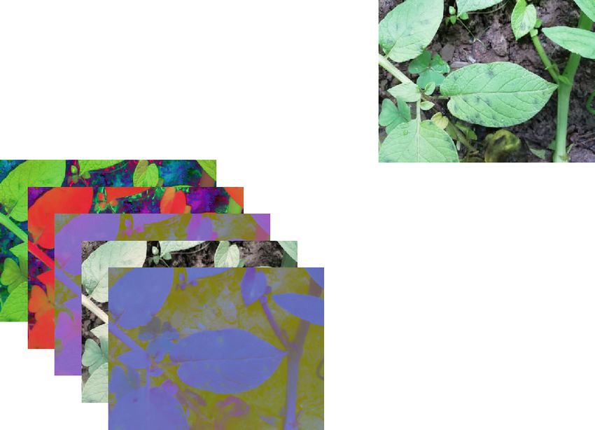
2 Plant Phenomics

illumination, focus, resolution, underlying feature size, and vide better representative features than the outline shape of
presence of occluding objects in the images. a leaf when considering the hierarchical transformation of
 More recently, the task of classification and detection in features from lower-level to higher-level abstraction for spe-
images has been dominated by various flavors of neural net- cies classes.
works (NNs), especially with the advent of deep NNs [9–14]. In addition to the choice of appropriate NN architectures,
It has been well-accepted that deep learning models perform preprocessing the image data can contribute towards obtain-
quite well in image classification and detection compared to ing better detection or classification. For example, it has been
traditional image-processing algorithms [15]. The process observed that a color spectrum provides better results than
of trial and error for fine-tuning traditional image processing grayscale for object detection by deep learning models [7]. A
models to obtain the representational features of objects color space or color model is a mathematical transformation
becomes rapidly complicated as the number of classes to project a set of primary colors to a different range of colors
increases. On the other hand, a neural network learns [27]. An investigation of the influence of different color spaces
complicated underlying patterns specific to a certain class to improve the deep learning model performance has been
of object without any manual intervention. A classification conducted for the traffic light detection system [28]. A com-
model using convolutional neural network (CNN) for distin- parative study for different color spaces using deep learning-
guishing 58 classes of healthy and diseased plant dataset was based automatic segmentation system has been discussed in
developed by Ferentinos and Konstantinos [16]. Arsenovic [29]. Disease region segmentation of paddy crop using
et al. [17] have improved the plant disease classification by Mask-RCNN on different color space images is analyzed in
increasing the training dataset, which has images of leaves [30]. Robustness and accuracy of the segmentation of foliar
in field conditions. Deep NNs have the potential to quickly disease spot images using region growth and comprehensive
detect an object from a complex image, which makes them color features have been explored in [31].
suitable for smart phone applications [7]. However, the train- The objective of this work is to develop a Mask R-CNN-
ing process in deep NNs is computationally expensive where based model to detect the blight symptoms on an infected
the network parameters are iteratively fine-tuned to improve potato leaf, which can eventually be deployed on a cell phone.
the mapping between a set of training input images and the Mask R-CNN [22] is chosen because it utilizes a feature pyr-
desired outputs [9]. Therefore, such methods have become amid network (FPN), allowing it to grasp semantically rele-
popular only with the concomitant advances in graphics pro- vant features at different resolution scales. The region
cessing hardware. proposal network (RPN) scans the entire top-bottom path-
 In the context of an image comprising a potato leaf way of the FPN for feature maps containing required objects
amidst a complex background, the classification process has and proposes regions of interest (ROI). This enables predic-
a binary outcome; i.e., it determines if the overall image tion of relevant classes, bounding boxes, and mask for the
reflects disease or not. Detection, on the other hand, goes region or patch. These methods of Mask R-CNN force differ-
one step further and demarcates the specific patch or patches ent layers in neural network to learn features across multiple
on the leaf that contain the signature of blight. Region-based scales, making it robust to several environmental variations
deep CNN (R-CNN) [18] is an object detection method that in the image. The model learns features from visual charac-
is trained to propose regions by exhaustively searching the teristics such as the shape, color, texture, and venation of a
image after it has been transformed through several convolu- potato leaf and blight disease for different training data.
tion layers. For the purpose of object detection, architectures The emphasis on detection rather than classification is
like YOLO [19], SSD [20], Faster R-CNN [21], and Mask because simple classification into healthy or unhealthy cate-
R-CNN [22] are recent methods, with Mask R-CNNs giving gories can be misleading due misclassification of soil patches
a better overall performance. For the R-CNN architectures, in the background as disease. To improve blight detection, we
the residual network with 50 layers (ResNet-50) is usually also investigate preprocessing the data to include different
used as a backbone. Other applications of CNN in agriculture color space images. Figure 1 conveys the overview of the
include Zhang et al. [23] who have used global pooling method proposed in this work. We have converted the RGB
dilated CNN for better segmentation and classification of color space dataset to five other color spaces, namely, HSL,
cucumber leaf disease, while CNN-based regression has been HSV, LAB, XYZ, and YCrCb and created a separate Mask-
used to estimate soybean leaf defoliation with the aid of real RCNN model for each color space. The model uses transfer
and synthetic images [24]. learning or stored knowledge of a pretrained Mask R-CNN
 The various transformations that an image undergoes as model on the Microsoft Common Objects in Context (MS
it traverses a deep CNN can sometimes be understood by COCO) dataset [32] as the initial condition for the training
visualizing the output of individual convolutional layers. process. The performance of the networks across the differ-
The output is termed as the feature map or activation map ent color spaces is compared in their ability to automatically
and can be visually correlated to the input image. Each con- detect infected potato leaves and disease patches in complex
volutional layer is a set of functions that applies some trans- field images.
formation to the image, behaving as a filter. The feature map
aids in relating the learned filter with the performance of the 2. Materials and Methods
model and using the learned filter to improve the perfor-
mance as discussed in [25]. Lee et al. [26] have reported such 2.1. Data Acquisition. The choice of data used for training a
studies in plants where the different orders of venation pro- CNN has a very strong impact of the effectiveness of the

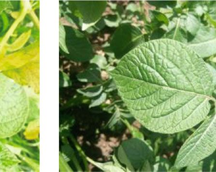
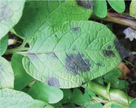
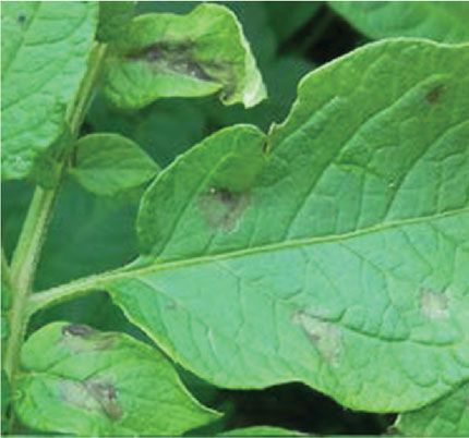
Plant Phenomics 3

 2. Color Space
 transformation

 HSL HSV
 LAB

 XYZ 1. Initial RGB
 dataset
 YCrCb

 RGB

 3. Deep-Learning based detection model 4. Result
 R-CNN Architecture
 Classification
 Feature Posterior
 extraction probability
 model Localization Detection

 Figure 1: Overview of the deep learning-based potato disease classification and detection method in this work.

 (a) (b) (c)

Figure 2: The complex background dataset used in this study: (a) multiple disease patches on a single leaf; (b) single disease patch on a
discolored leaf; (c) healthy leaves.

model in different situations. Factors such as the characteris- cellular phones. Therefore, the potato leaf dataset contains
tics of the imaging sensor, the imaging protocol followed, images of resolutions of 3072 × 4096 pixels (552 images),
illumination variation due to time of the day, shadows due 3120 × 4160 pixels (922 images), and 2448 × 3264 pixels
to nearby objects, occlusion, and complex background infor- (366 images) due to inherent differences in the sensors of
mation all need to be carefully considered to create a model the different smart phones used for data collection.
that can be successfully applied to field-based imaging. In The images are heterogeneous, having been taken from
order to maximize the diversity of training data, a set of different locations within the field at different times of the
1840 field-based images of potato leaves was acquired for day, typically between 11 am and 2 pm. Each image can con-
this work across different states in India by field personnel tain several leaves, soil, and weeds in the background apart
deputed under the FarmerZone project [33]. from the primary infected/healthy potato leaf. This variation
 The dataset comprises images of healthy potato leaves as aids the generalization of the deep learning model. All images
well as leaves affected by both early and late blights. As one of were captured in natural light with the camera flash always
the objectives was to develop a model that would be accessi- turned off and without any additional optical or digital zoom.
ble to a larger group of small-scale farmers, it was determined Sample images of healthy leaves and leaves affected with
that the choice of imaging sensors should include low-end blight are shown in Figure 2.

4 Plant Phenomics

2.2. Data Curation. The potato leaf images obtained using Table 1: Description of manually annotated patches for different
smart phones are in the RGB format, which is similar to the features in the dataset.
human perception of the light spectrum as a combination
 Data Train Test Total
of the primary colors—red, green, and blue [34]. While there
is potential for improved image segmentation using other No. of images 1423 417 1840
color spaces, there is no general opinion on the best choice No. of blight patches 4673 1152 5825
of color space for image segmentation. Therefore, all the No. of infected leaves 1423 356 1779
RGB images were converted to five color spaces (HSV, No. of healthy leaves 122 89 211
HSL, XYZ, LAB, and YCrCb) using Open Computer Vision
Library [35], creating additional 5 datasets. In the RGB data-
set, one or more blight spots on each potato leaf in the fore- an identity function before the final ReLU activation func-
ground are manually demarcated into patches for creating tion. It is observed that during backpropagation, larger gradi-
the ground-truth dataset. The process of demarcating or seg- ents are available for initial layers leading to faster learning
menting the images was carried out by three personnel, two because of skip or residual connection. ResNet-50 has 50
nonexperts under the guidance of an agricultural expert. layers arranged in five stages with a total of sixteen residual
The ground-truth values and labels are kept the same for all blocks. In each residual block, the convolutional layer is
the images in different color space datasets. To reduce the followed by a batch normalization layer and a ReLU activa-
annotator’s bias and variance [36] during ground-truth tion function. The ResNet-50 model generates 256, 512,
annotation, the following steps were taken: 1024, and 2048 feature maps from the second, third, fourth,
 and fifth stages, respectively.
 (i) The expert first demonstrated the protocol for seg- Each color space dataset is used for training a separate
 mentation of patches on foreground, the edges to be Mask R-CNN detection model. In a preprocessing step, the
 considered, and how tightly the polygon should be input images are downsampled to 1024 × 1024 pixels. For
 drawn each color space model, the mean value of each channel of
 the respective color space, calculated separately from the
 (ii) For 50 randomly selected images, the expert and the training dataset, is set in the configuration file of the program
 nonexperts all annotated according to the prescribed [38]. Pretrained weights of the MS COCO dataset have been
 procedure. The value of Cohen’s kappa [37] found used for the initial training of the model as attempts to train
 across the three annotators was 0.92, and level of from scratch did not yield significant detection even after
 agreement was found to be very good. Thereafter, 70th epoch for all of the color space datasets, probably due
 5825 blight patches, 1779 infected leaf patches, and to the small dataset. On the other hand, the application of
 211 healthy leaf patches were created from the 1840 transfer learning towards classification of potato leaf disease
 input images. Table 1 provides the details of the total was shown in [39, 40]. To optimize the network weights,
 dataset and its annotation count. To create and vali- the stochastic gradient descent optimizer with momentum
 date the disease detection model, the dataset of each fixed at 0.9 was used. A fixed learning rate of 1e-4 was set
 color space was further split into 2 sets containing for optimum learning. The maximum number of epochs
 approximately 80% and 20% data, respectively was set to 100, and iterations per epoch were set to 712 cor-
 responding to a batch size of two images per iteration.
2.3. Mask R-CNN-Based Detection Model. The detailed block
diagram of Mask R-CNN used in this work is shown in 2.4. Computing Resources Utilized. The training and testing
Figure 3. Mask R-CNN is an extension of Faster R-CNN of the model were performed on a CentOS 7 Linux worksta-
[38], with an additional forking to a prediction segmentation tion equipped with one Intel Xeon Processor CPU (96 GB
mask on each RoI, in parallel with the already available RAM), accelerated by one Nvidia GeForce GTX 1080 Ti
branch for classification and bounding box regression. In this GPU (11GB Memory). The model is implemented in the
work, further tuning of the original Mask RCNN includes the Keras 2.2.4 deep learning open-source framework with the
use of ResNet-50 as backbone architecture with RPN anchor TensorFlow-GPU 1.8.0 backend using Python 3.6. The detec-
scales set to 32, 64, 128, 256, and 512 and the anchor aspect tion model on each color space took an average of 25 hours
ratios set to 1 : 2, 1 : 1, and 2 : 1. This follows from manual for training.
observation of the training dataset, which shows that the var- For creating the ground-truth dataset VGG Image Anno-
ious demarcated patches vary in this selected range of pixel tator (VIA) [41], a standalone software was used for the
values and aspect ratios. manual annotation of the blight and leaf patches in the
 Regarding the choice of ResNet-50 as the backbone, it image. It allows a rectangular- and polygonal-shaped area
may be noted that deep CNN is prone to problems like van- to be annotated, which is useful for training Mask R-CNN.
ishing gradients and the curse of dimensionality [14], with an
increase in the number of layers. To avoid this degradation 2.5. Model Evaluation Metrics. In computer vision, standard
problem for a deeper network, skip connections (identity metrics like precision and recall are used for performance
connections) or residual connections are used. The residual evaluation of binary classification [42]. This is obtained from
connection is a “shortcut” module, whereby the weight/con- a confusion matrix that summarizes the performance of a
volutional layers are skipped and the input is added through classifier for a given test dataset. The four components of

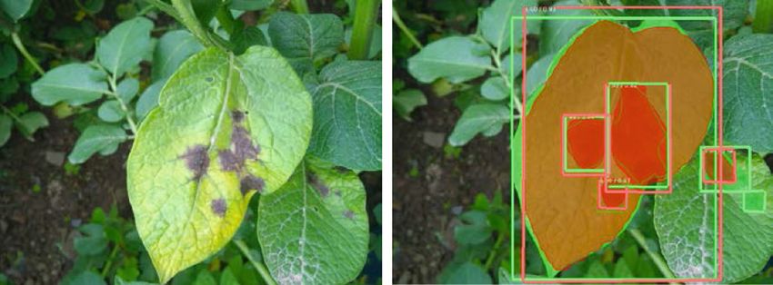
Plant Phenomics 5

 Mask R-CNN detection model

 Bounding box
 CNN

 regression
 Fully connected layer
 RoI align

 Residual network
 Fixed size
 feature map

 Classification
 Feature map Mask branch

 ResNet - 50
 RPN

 Figure 3: Block diagram of a model architecture for the implemented Mask R-CNN models.

 Figure 4: An example to describe IoU on the object with and without annotation.

the 2 × 2 confusion matrix for any binary classifier are true represent the human-annotated ground truth while red color
positive (TP), true negative (TN), false positive (FP), and masks and bounding boxes represent the predictions by the
false negative (FN). The correct classification of an image detection model. For the sample image shown in Figure 4,
containing disease would count as a TP, while an incorrect the confidence score and IoU for the infected leaf are 100%
classification as a healthy image would count as a FP. The and 93%, respectively.
performance of the classifier is then obtained by In addition to the boundaries of the PI, the algorithm also
 provides a confidence level for the PI. The AP is a metric that
 TP TP incorporates the confidence level of prediction and IoU into
 Precision = Recall = : ð1Þ
 TP + FP TP + FN the calculation of precision using the area under precision-
 recall curve. Mean average precision (mAP) is mean of AP
 For the performance assessment of the object detection across the different categories or classes, which are detected,
model, both the correct classification and the precise location and summarizes the performance of a detection model.
of the disease patch in the image should be taken into
account. To do so, concepts such as intersection over union
(IoU) and the average precision (AP) were introduced in
 3. Results and Analyses
the Pascal VOC challenge [43]. The IoU metric determines 3.1. Disease Detection. The performance of the disease detec-
the correctness of the patch detection by taking into account tion model, when tested on the ground-truth potato leaf
how closely the predicted instance (PI) fits the ground-truth dataset, is calculated according to the metrics defined in Sec-
instance (G). IoU is the measure of overlap between G and PI tion 2.5. A separate model is created for each color space.
boundaries given by Even within each color space, there are two types of Mask
 R-CNN models:
 G ∩ PI
 IoUðG, PIÞ = : ð2Þ
 G ∪ PI (i) Two-class model: this involves the detection of only
 potato blight patches, while the rest of the image is
 The IoU threshold is taken to be 0.5 as a common prac- considered as background. This kind of demarcation
tice, whereby if the IoU value of detection is greater than is a natural first step where it is expected to detect
0.5, then the PI is considered as a TP, or else it is taken as a only blight disease patches from the input image.
FP. This is illustrated using a sample test image shown in However, once the model was trained over the entire
Figure 4, where green color masks and bounding boxes dataset, it was found that several blight patches were

6 Plant Phenomics

 (a) (b)

 Figure 5: (a) Sample test RGB image and (b) output image for the trained two-class Mask R-CNN model.

 (a) (b)

 Figure 6: Sample RGB image: (a) human annotated foreground regions; (b) patches inferred by the 4-class HSL model.

 (a) (b)

 Figure 7: Sample RGB image: (a) with annotated foreground regions; (b) patches inferred by the 4-class RGB model.

 not detected and that a few soil patches were misclas- For both models, the ground-truth criteria were kept
 sified as blight. A sample test image from the RGB uniform for all the images. The aim of this second model
 dataset (Figure 5(a)) contains nine disease patches was to increase blight disease patch detection and reduce
 spread across three different leaves. Figure 5(b) the FP due to misclassification of soil as disease, by the inclu-
 shows that the two-class model has detected only sion of a postprocessing step that checks for the intersection
 two disease patches out of nine clearly distinguish- of the disease patch with the leaf patch. Nevertheless, it was
 able disease patches seen that the performance of the four-class model was
 superior to that of the two-class model even without any
 (ii) Four-class model: as a means to improve the perfor- additional postprocessing. The performance scores for the
 mance of the detection model, a second experiment 2-class and the 4-class detection models are compared in
 was performed in which the Mask R-CNN model Table 2 with respect to different color spaces.
 was trained to detect 4 classes: blight disease patches, Among the two-class Mask R-CNN models for different
 infected leaves, and healthy leaves, in addition to the color spaces, LAB color space has the best mAP (80.1%)
 background (Figures 6 and 7). and mAR (55.6%) values. The 4-class detection model shows

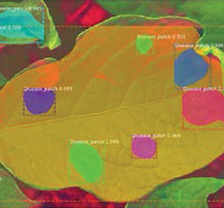
Plant Phenomics 7

 Table 2: Performance of various color spaces compared to RGB for potato disease detection.

 2-class detection model 4-class detection model
Color space Avg. inference time/image (sec)
 mAP (%) mAR (%) mAP (%) mAR (%)
RGB 77.4 53.9 80.9 55.5 1.77
XYZ 77.4 54.2 70.8 52.9 1.68
HSL 78.2 55.2 81.3 56.9 1.67
HSV 75.5 53.9 75.5 55.4 1.67
LAB 80.1 55.6 81.4 56.4 1.68
YCrCb 76.1 54.3 79.1 56.4 1.70
Performance score calculated for IoU = 0:5.

 Table 3: Manually obtained performance metrics of the four-class Mask R-CNN model.

 Disease patch Infected leaf Healthy leaf Combined
Color space
 TP1 TP2 FN FP TP FN FP TP FN FP P (%) R (%)
RGB 375 166 176 7 329 22 10 93 15 2 98.1 81.9
XYZ 343 191 173 1 340 11 34 52 55 1 96.3 79.5
HSL 464 159 147 5 338 13 21 83 25 2 97.5 85.0
HSV 428 149 140 7 341 10 23 68 40 1 96.9 83.8
LAB 395 175 180 2 333 18 11 91 17 1 98.6 82.2
YCrCb 394 253 101 9 336 15 30 52 56 0 96.4 85.8

a slightly improved mAP (LAB) and mAR (HSL) perfor- eters, despite the correct classification by the model.
mance metrics of 81.4% and 56.9%, respectively. It was Hence, the ground-truth annotation might need to be
observed that HSL, LAB, and YCrCb color space models more inclusive of disease patches to better represent the
could perform better than RGB color space model overall performance score.
and specifically for disease patch detection. Inference times
are the least for the detection model trained on HSL and 3.2. Manual Analysis of the Detection Model. Considering the
HSV color spaces. These results are in line with the latest challenges of ground-truth labeling, we attempted a more
leaderboard on the COCO website [44], which publishes realistic quantification of disease patch detections by manu-
the performance results for different models on the COCO ally verifying the outputs of the 4-class model (Table 3).
dataset with 91 categories. The highest mAP (IoU = 0:5) is The correct disease patch predictions were categorized into
60.6% for a model trained on the dataset of broccoli category two true-positive categories: TP1 reflects the correct detec-
(closest to potato leaves). tions that match the ground truth while TP2 reflects correct
 Further investigation into the performance of different disease detections that have not been annotated in the
four-class detection models by manually comparing the test ground truth. The same exercise is carried out for the infected
image data to the model outputs shows that the performance leaf and healthy leaf classes also. Table 3 summarizes the
of the disease detection model appears far better than the results of manually determining the detection performance
mAP and mAR values reported in Table 2. This surprising on the test dataset, for all color spaces. It can be inferred
outcome can be understood if we delve into the ground- that among the six color space models, the model trained
truth labeling procedures. The images taken from the field on HSL color space has the best disease detection with 464
have many complex regions due to fuzziness of image, par- (TP1) patches detected. The LAB and YCrCb color space
tially occluded disease patches, and disease patches on the trained models have the best combined four-class perfor-
stem. Many disease patches that fall into these categories mance metrics of 98.6% (combined precision) and 85.8%
were not annotated while creating the ground-truth dataset. (combined recall), respectively. The YCrCb model shows
Also, for the human annotator, there is often no clear distinc- maximum true disease detection (TP1 + TP2) of 647 dis-
tion between the foreground and background features, ease patches. The infected leaf patches were detected better
whether for disease patches or the leaves. The human anno- by the HSV color space model with 341 true detections. It
tator, for example, has annotated (shaded region shown in was observed that HSL, HSV, LAB, and YCrCb models
Figures 6(a) and 7(a)) only clearly distinct features of disease performed better than the RGB color space model for
or leaf patches. However, our trained models have correctly the detection of disease patch and infected leaf. In all color
predicted several unlabeled disease patches in the back- space instances of the 4-class model, very few FP are
ground as disease (Figures 6(b) and 7(b)). Since these “vague” observed for disease patch class while most of the FP in
disease patches have not been labeled in the ground-truth the infected leaf class are misclassifications of a healthy
dataset, they end up lowering the mAP and mAR param- leaf.

8 Plant Phenomics

 Color space with Boxplot for pixel intensity distribution Channel
 Region
 sample image Disease (D) Soil (S) leaf (L) 1 2 3
 250
 95 188 146

 L
 200
 45.6 36.9 46.8
 150
 68 99 98

 S
 100
 37.5 51.4 48.2
 50
 101 151 144

 D
 RGB 0
 46.9 49.4 48.8
 250
 130 165 165

 L
 200
 35.6 36.2 47.7
 150
 77 92 102

 S
 100
 40.1 46.3 51.7
 50
 120 140 155

 D
 XYZ 0
 41.9 45.9 52.0
 250
 75 141 125

 L
 200
 11.3 37.3 48.2
 150
 91 82 65

 S
 100
 19.4 42.8 49.0
 50
 85 130 82

 D
 HSL 0
 20.4 44.3 52.3
 250
 75 127 188

 L
 200
 11.3 37.3 48.2
 150
 91 82 101

 S
 100
 19.4 42.8 49.0
 50
 85 99 159
 HSV 0 D 20.4 44.3 52.3
 250
 125 94 140
 L

 200
 34.2 9.8 12.7
 150
 100 123 126
 S

 100
 49.7 13.5 11.4
 50
 150 112 127
 D

 LAB 0
 46.4 13.9 12.2
 250
 156 86 124
 L

 200
 36.5 18.4 14.0
 150
 76 115 131
 S

 100
 44.6 14.9 9.1
 50
 140 103 133
 D

 YCrCb 0
 45.0 18.1 11.4

Figure 8: Sample image and box plot of the pixel intensities of the three channels for each color space, for the disease, soil, and leaf patches
(channel 1, channel 2, and channel 3 are represented by red, green, and blue color, respectively in the box plots). Mean (μ) and standard
deviation (σ) corresponding to the box plots are also provided for numerical comparison.

3.3. Analysis of the Role of Color Spaces. Hadji et al. [45] have contained 102 patches, and patches that did not meet the pre-
previously shown that the histogram of image intensities is determined patch size and features were discarded. The pixel
used broadly for recognition and retrieval in an image data- intensity distribution for patches of disease (D), soil (S), and
base. For a better understanding of the effect of each color leaf (L) regions in the form of a box plot with the mean (μ)
space on the potato leaf dataset, the histogram trends of var- and the standard deviation (σ) for each channel of the color
ious color components in the image can be observed [46]. space is shown.
Figure 8 shows a histogram analysis on thirty randomly It is observed from Figure 8 that each of the channels of
selected potato leaf images with blight symptoms. Each the RGB color space shows pixel distribution with a large
image was of 2448 × 3264 pixels and further divided into spread that overlaps with the adjacent regions. This is due
image patches of 200 × 200 pixels. All patches were manually to varying illumination conditions across images, which
labeled into classes of blight disease, healthy leaf, soil, and equally affect the R, G, and B channels. Only for channel 2
background. The count of patches for each class was as fol- is there some separation between the distribution of disease
lows: the blight disease class contained 844 patches, the and leaf regions. This color information might be used by a
healthy leaf class contained 2216 patches, the soil class deep learning model for classification. Similar to the RGB

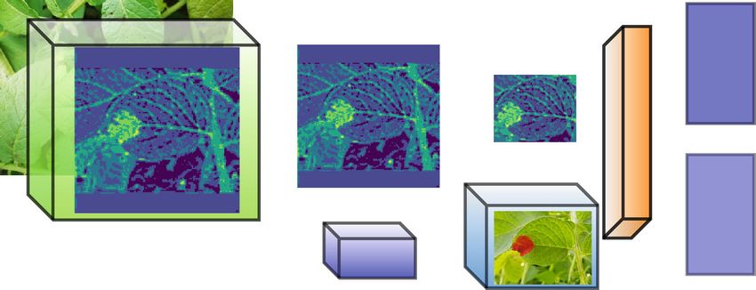
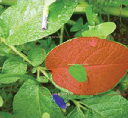
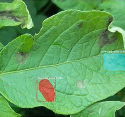
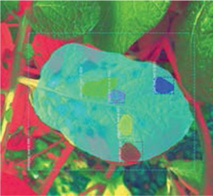
Plant Phenomics 9

 (a) (b) (c)

Figure 9: (a) Sample output image, corresponding visualization of the leaf, and disease-relevant feature map for (b) 2c and (c) 5c layers of the
RGB color space detection model.

color space, the XYZ color space has a wide distribution of maps of the different stages of ResNet, trained for four-class
intensity values for all the components. Here, channel 2 has detection include a number of relevant ones showing features
better separation between soil and leaf regions. of leaves and disease patches. Figure 9(a) shows the sample
 Conversion to HSL from RGB color space restricts the output image for the RGB color space detection model.
range of certain components such as hue, which are illumina- Figures 9(b) and 9(c) both show the visualization of the leaf
tion independent. Therefore, the hue component is expected feature and disease patch feature side-by-side for the 2c and
to have a narrow range for all regions. Thus, it can be the 5c layer, respectively. From Figure 9, it was inferred that
observed that although each of the HSL channels’ distribu- the leaf features are well learned. The activation in the 5c
tion overlaps across all regions, the overlap is minimum for layer shows that along with features of disease patch, features
the hue channel. The many outliers might still make classifi- of soil patch have also been learned by the detection model.
cation difficult using only hue information. Similar to HSL, Overall, the 36th, 12th, 31th, and 28th feature maps of the 2nd
the HSV color space has the same hue information. Com- to the 5th layers were strongly related to disease, flower in
pared to HSL, the HSV has more spread in pixel intensity dis- the background, infected leaf, and healthy leaf, respectively.
tribution for channels 2 and 3. This might lead to reduced The learning of leaf venation could be properly observed in
performance of the detection model. In the case of LAB, the feature maps.
channel 1 (lightness) varies according to lighting conditions. It is interesting to observe that for the model trained with
The component a ∗ and b ∗, represented by green and blue HSL color space dataset, learning and extraction of the finer
boxes, respectively, are the green–red component and a leaf and disease patch features were observed in the visualiza-
blue-yellow component of the image. From Figure 8, it can tions for the second to the fifth stage of the model. From the
be observed that a∗ and b∗ components have a narrow range leaf feature maps, it could be inferred that a leaf’s feature is
of pixel intensity values. Here, the a∗ component shows sep- better learned when it is in proper camera focus. The feature
aration in values for leaf, soil, and disease regions. Similarly, maps for the sample HSL output image are shown in
the b∗ component has a very narrow overlapping area. This Figure 10(a) with the fourth and the fifth stages shown in
clear segregation in the a∗ and b∗ components could help Figures 10(b) and 10(c). Here, the diseased patch is clearly
in better classification and detection models. For the case of learned apart from the background or the soil patches.
YCrCb, blue-difference chroma and red-difference chroma Similar to HSL, the HSV color space detection model has
have narrow spreads for different regions. The red box repre- learned the leaf venation and disease patch structures clearly,
sents the luma component; green and blue boxes represent which are visible in all the leaf feature maps of different stages
blue and red-difference chroma, respectively. In channel 2, for the model shown in Figures 11(b) and 11(c). Here, a total
the soil and the leaf regions are distributed apart from each of 54 and 43 feature maps have a strong correlation with the
other while all other channels overlap in their distributions diseased patch and leaf feature, respectively.
for the different regions. Thus, the histogram analysis helps The sample LAB color space image shows that the disease
to understand the color complexity of different patches/ patch (dark-blue color mask), the infected leaf (green color
regions and it is observed that the color information will mask), and the healthy leaf (red color mask) have all been
solely not lead to good segmentation between disease, soil, detected. From the feature maps shown in Figure 12(a), it is
and leaf regions. Higher-level features like the texture of the observed that the diseased patch, the infected leaf, and the
disease region and leaf venation will need to be used by the healthy leaf features are learned separately. The YCrCb color
deep learning model for segmentation, in addition to color. space model detects the various classes similar to the LAB
 color space model with a sharp distinction between the three
3.4. Feature Map Observations. The characterization of blight classes.
disease, soil, and leaf regions by the CNN can be observed
from the deconvolutional layers. The deconvolutional net- 4. Discussion
work maps the feature activity back to the input pixel space
by using the same components of the convolutional layer The primary aim of this work is to deliver blight advisories to
(filtering, pooling) in the reverse order [25, 26]. The feature potato farmers in a timely and automated manner. As blight

10 Plant Phenomics

 (a) (b) (c)

Figure 10: (a) Sample output image, corresponding visualization of the leaf, and disease-relevant feature map for (b) 4c and (c) 5c layers of
the HSL color space detection model.

 (a) (b) (c)

Figure 11: (a) Sample output image, corresponding visualization of the leaf, and disease-relevant feature map for (b) 2c and (c) 4c layers of
the HSV color space detection model.

 (a) (b) (c)

Figure 12: (a) Sample output image, corresponding visualization of the leaf, and disease-relevant feature map for (b) 2c and (c) 3c layers of
the LAB color space detection model.

spreads fairly rapidly, farmers are advised to spray fungicide color models, one may easily create a consensus system using
as soon as blight occurrence is detected. Therefore, in addi- multiple color models in parallel, to further enhance the
tion to successfully detecting true occurrences of blight, the detection. This kind of software and algorithmic approach
blight model should also minimize the number of false- to processing RGB images can be far more cost-effective than
positive detections. Otherwise, it can lead to unnecessary the use of multispectral or hyperspectral cameras. Also, RGB-
spraying of fungicide and higher input costs to farmers. False based data acquisition and analyses are transferable to smart
positives can be a problem when using simple binary classifi- phones that are usually affordable to farmers.
cation since the model might misinterpret the background The underpinnings of any successful detection model are
soil patches as occurrences of blight and give a false alarm. the quality and quantity of training data. Image data in par-
Therefore, both a 2-class detection model and a 4-class detec- ticular can vary greatly in field environments due to occlu-
tion model are explored in this work. sions of the disease regions due to neighboring leaves or
 The use of various color space transformations for pre- stems; out-of-focus target regions due to movement of the
processing the data enables higher detection accuracy by cir- sensor or the target leaves themselves; illumination variation
cumventing the variations in lighting conditions on the field. due to the season, time of the day, and angle of imaging; and
While this work has presented the performance of individual morphological variations of leaves in terms of size, shape,

Plant Phenomics 11

and texture. Therefore, a significant contribution of this work work could be extended to gauge the disease severity by
is in the collection of diverse field images of potato across dif- quantifying the number and the size of blight disease patches
ferent geographies and time instants to ensure a heteroge- per leaf.
neous training data.
 Modern cell phone cameras have improved in their imag- Data Availability
ing capability along with the software-enhanced image pro-
cessing offered by such phones. The acquisition of data All data used to train and test the model presented in this
using a variety of cell phones might lead to a model that paper is freely available upon request.
can find wide applicability when many farmers are hesitant
to adopt/invest in aerial or ground-based phenotyping equip-
ment. Apart from model performance, inference time and Conflicts of Interest
memory space utilization are also important metrics for SS is an advisor to Arnetta Technologies Pvt. Ltd, a startup
smart phone application. Therefore, the challenge will be to venturing into breeding management systems for cereal
reduce the model size, while retaining its performance. Infer- crops. The authors declare that there is no conflict of interest
ence from a single image presently takes about 1-2 seconds, regarding the publication of this article.
which makes it of practical value.
 In practice, the farmer will need alerts of even a single
occurrence of blight to contain it in the initial stage. In this Authors’ Contributions
context, it may be noted that the mAP and mAR scores pro-
 JJ carried out the simulations and generated the results with
vided in Table 3 are quite conservative due to the underlying
concept of IoU. While evaluating the performance of the assistance from GS. GS curated and annotated the datasets.
 SS conceived, designed, and supervised the work. JJ and SS
model, a detection is considered correct only if the model is
 wrote the manuscript. S. Sharma and JS supervised the anno-
able to place a bounding box around the disease that has at
 tation and classification of diseases. SKM and VKD super-
least 50% area of intersection with a ground-truth box
 vised the data management and testing.
demarcated by an expert. While this provides good standard-
ization for model evaluation across various application
domains, it may be noted that in the context of disease detec- Acknowledgments
tion, the performance of the model is gauged depending on
how the expert annotates the ground truth. Figure 8, on the The authors express their gratitude to Dr. Sanjay Rawal, Dr.
other hand, gives a more liberal interpretation of the model Prince Kumar, Portia D Singh, Krishan Kumar, Mahesh
performance by testing how well the model can demarcate Vikal, Kawalpreet, and Harish Kumar for data collection
the disease without reference to the specific ground truth and management. This research was supported by the
annotations. Thus, the results presented in Figure 8 show that Government of India’s Department of Biotechnology under
the model presented in this work can lead to more optimistic the FarmerZone™ initiative (# BT/IN/Data Reuse/2017-18)
outcomes for the potato farmer. and the Ramalingaswami Re-entry fellowship (# BT/RLF/
 Re-entry/44/2016).
5. Conclusions
 References
This work has demonstrated a potato blight detection model
using the deep learning approach that can be applied in field [1] R. K. Arora, S. Sharma, and B. P. Singh, “Late blight disease of
conditions, for aiding the farmer in making real-time deci- potato and its management,” Potato Journal, vol. 41, no. 1,
sions. In order to improve the detection performance of the pp. 16–40, 2014.
model on data acquired from easily available RGB sensors, [2] A. J. Haverkort, P. C. Struik, R. G. F. Visser, and E. J. P. R.
the input data are mathematically transformed to other color Jacobsen, “Applied biotechnology to combat late blight in
spaces to aid the training of the Mask R-CNN model. It is potato caused by Phytophthora infestans,” Potato Research,
 vol. 52, no. 3, pp. 249–264, 2009.
observed that training in the LAB color space provides the
highest performance metrics with 80.1% and 81.4% mAP [3] M. Islam, A. Dinh, K. Wahid, and P. Bhowmik, “Detection of
 potato diseases using image segmentation and multiclass sup-
for the 2-class and 4-class detection models, respectively.
 port vector machine,” in 2017 IEEE 30th Canadian Conference
The XYZ color space has the lowest mAP values for both on Electrical and Computer Engineering (CCECE), pp. 1–4,
detection models, yielding 77.4% and 70.8%, respectively. Windsor, ON, Canada, April-May 2017.
However, the model can provide an optimistic performance [4] A. Vibhute and S. K. Bodhe, “Applications of image processing
of ~98% overall precision for disease detection in the real- in agriculture: a survey,” International Journal of Computer
world scenario. The feature maps of intermediate layers of Applications, vol. 52, no. 2, pp. 34–40, 2012.
the trained detection models were observed, and it was found [5] J. G. A. Barbedo, “Plant disease identification from individual
that color spaces with better performance enabled the model lesions and spots using deep learning,” Biosystems Engineering,
to learn fine features of the disease patch, the leaf patch, and vol. 180, pp. 96–107, 2019.
the soil patch such as color, texture, leaf venation, and leaf [6] S. Parkes and S. Teltscher, I.C.T Facts and Figures-the World in
shape. The inference time per image and size of the detection 2015, The International Telecommunication Union (ITU),
models allow quick response when deployed in the field. This Geneva, 2015.

12 Plant Phenomics

 [7] S. P. Mohanty, D. P. Hughes, and M. Salathé, “Using deep [23] S. Zhang, C. Zhang, X. Wang, and Y. Shi, “Cucumber leaf dis-
 learning for image-based plant disease detection,” Frontiers ease identification with global pooling dilated convolutional
 in Plant Science, vol. 7, article 1419, 2016. neural network,” Computers and Electronics in Agriculture,
 [8] S. Biswas, B. Jagyasi, B. P. Singh, and M. Lal, “Severity identi- vol. 162, pp. 422–430, 2019.
 fication of potato late blight disease from crop images captured [24] L. A. da Silva, P. O. Bressan, D. N. Gonçalves, D. M. Freitas,
 under uncontrolled environment,” in 2014 IEEE Canada Inter- B. B. Machado, and W. N. Gonçalves, “Estimating soybean leaf
 national Humanitarian Technology Conference - (IHTC), defoliation using convolutional neural networks and synthetic
 pp. 1–5, Montreal, QC, Canada, June 2014. images,” Computers and Electronics in Agriculture, vol. 156,
 [9] A. Krizhevsky, I. Sutskever, and G. E. Hinton, “Imagenet pp. 360–368, 2019.
 classification with deep convolutional neural networks,” [25] M. D. Zeiler and R. Fergus, “Visualizing and understanding
 Communications of the ACM, vol. 60, no. 6, pp. 84–90, convolutional networks,” in Computer Vision – ECCV 2014.
 2017. ECCV 2014. Lecture Notes in Computer Science, vol 8689, D.
[10] Y. Toda and F. Okura, “How convolutional neural networks Fleet, T. Pajdla, B. Schiele, and T. Tuytelaars, Eds., pp. 818–
 diagnose plant disease,” Plant Phenomics, vol. 2019, article 833, Springer, Cham, 2014.
 9237136, pp. 1–14, 2019. [26] S. H. Lee, C. S. Chan, S. J. Mayo, and P. Remagnino, “How
[11] Y. LeCun, L. Bottou, Y. Bengio, and P. Haffner, “Gradient- deep learning extracts and learns leaf features for plant classi-
 based learning applied to document recognition,” Proceedings fication,” Pattern Recognition, vol. 71, pp. 1–13, 2017.
 of the IEEE, vol. 86, no. 11, pp. 2278–2324, 1998. [27] N. A. Ibraheem, M. M. Hasan, R. Z. Khan, and P. K. Mishra,
[12] K. Simonyan and A. Zisserman, “Very deep convolutional net- “Understanding color models: a review,” ARPN Journal of Sci-
 works for large-scale image recognition,” 2014, http://arxiv ence and Technology, vol. 2, 2012.
 .org/abs/1409.1556. [28] H. K. Kim, J. H. Park, and H. Y. Jung, “An efficient color space
[13] C. Szegedy, W. Liu, Y. Jia et al., “Going deeper with convolu- for deep-learning based traffic light recognition,” Journal of
 tions,” in 2015 IEEE Conference on Computer Vision and Pat- Advanced Transportation, vol. 2018, Article ID 2365414, 12
 tern Recognition (CVPR), pp. 1–9, Boston, MA, USA, June pages, 2018.
 2015. [29] D. Khattab, H. M. Ebied, A. S. Hussein, and M. F. Tolba,
[14] K. He, X. Zhang, S. Ren, and J. Sun, “Deep residual learning for “Color image segmentation based on different color space
 image recognition,” in 2016 IEEE Conference on Computer models using automatic GrabCut,” The Scientific World Jour-
 Vision and Pattern Recognition (CVPR), pp. 770–778, Las nal, vol. 2014, Article ID 126025, 10 pages, 2014.
 Vegas, NV, USA, June 2016. [30] S. Das, D. Roy, and P. Das, “Disease feature extraction and dis-
[15] N. O’Mahony, S. Campbell, A. Carvalho et al., “Deep learning ease detection from paddy crops using image processing and
 vs. traditional computer vision,” in Advances in Computer deep learning technique,” in Computational Intelligence in
 Vision. CVC 2019. Advances in Intelligent Systems and Com- Pattern Recognition. Advances in Intelligent Systems and Com-
 puting, vol 943, K. Arai and S. Kapoor, Eds., pp. 128–144, puting, vol 1120, A. Das, J. Nayak, B. Naik, S. Dutta, and D.
 Springer, Cham, 2019. Pelusi, Eds., pp. 443–449, Springer, Singapore, 2020.
[16] K. P. Ferentinos, “Deep learning models for plant disease [31] J. Ma, K. Du, L. Zhang, F. Zheng, J. Chu, and Z. Sun, “A seg-
 detection and diagnosis,” Computers and Electronics in Agri- mentation method for greenhouse vegetable foliar disease
 culture, vol. 145, pp. 311–318, 2018. spots images using color information and region growing,”
 Computers and Electronics in Agriculture, vol. 142, pp. 110–
[17] M. Arsenovic, M. Karanovic, S. Sladojevic, A. Anderla, and
 117, 2017.
 D. Stefanovic, “Solving current limitations of deep learning
 based approaches for plant disease detection,” Symmetry, [32] T. Y. Lin, M. Maire, S. Belongie et al., “Microsoft coco: com-
 vol. 11, no. 7, p. 939, 2019. mon objects in context,” in Computer Vision – ECCV 2014.
 ECCV 2014. Lecture Notes in Computer Science, vol 8693, D.
[18] R. Girshick, J. Donahue, T. Darrell, and J. Malik, “Rich feature
 Fleet, T. Pajdla, B. Schiele, and T. Tuytelaars, Eds., pp. 740–
 hierarchies for accurate object detection and semantic segmen-
 755, Springer, Cham, 2014.
 tation,” in 2014 IEEE Conference on Computer Vision and Pat-
 tern Recognition, pp. 580–587, Columbus, OH, USA, June 2014. [33] Farmerzone-website, 2018, http://www.farmerzone.in/.
[19] R. Joseph, S. Divvala, R. Girshick, and A. Farhadi, “You only [34] K. N. Plataniotis and A. N. Venetsanopoulos, Color Image Pro-
 look once: unified, real-time object detection,” in 2016 IEEE cessing and Applications, Springer Science & Business Media,
 Conference on Computer Vision and Pattern Recognition 2013.
 (CVPR), pp. 779–788, Las Vegas, NV, USA, June 2016. [35] OpenCV, Color conversions, 2017, https://docs.opencv.org/3.4
[20] L. Wei, D. Anguelov, D. Erhan et al., “SSD: single shot multi- .0/de/d25/imgproccolorconversions.html.
 box detector,” in Computer Vision – ECCV 2016. ECCV [36] T. A. Lampert, A. Stumpf, and P. Gançarski, “An empirical
 2016. Lecture Notes in Computer Science, vol 9905, B. Leibe, J. study into annotator agreement, ground truth estimation,
 Matas, N. Sebe, and M. Welling, Eds., pp. 21–37, Springer, and algorithm evaluation,” IEEE Transactions on Image Pro-
 Cham, 2016. cessing, vol. 25, no. 6, pp. 2557–2572, 2016.
[21] S. Ren, K. He, R. Girshick, and J. Sun, “Faster R-CNN: towards [37] M. L. McHugh, “Interrater reliability: the kappa statistic,” Bio-
 real-time object detection with region proposal networks,” chemia Medica, vol. 22, no. 3, pp. 276–282, 2012.
 IEEE Transactions on Pattern Analysis and Machine Intelli- [38] Y. Kim, FasterRCNN, 2017, https://github.com/you359/Keras-
 gence, vol. 39, no. 6, pp. 1137–1149, 2017. FasterRCNN.
[22] K. He, G. Gkioxari, P. Dollar, and R. Girshick, “Mask R-CNN,” [39] F. Islam, M. N. Hoq, and C. M. Rahman, “Application of trans-
 in 2017 IEEE International Conference on Computer Vision fer learning to detect potato disease from leaf image,” in 2019
 (ICCV), pp. 2980–2988, Venice, Italy, October 2017. IEEE International Conference on Robotics, Automation,

Plant Phenomics 13

 Artificial-intelligence and Internet-of-Things (RAAICON),,
 pp. 127–130, Dhaka, Bangladesh, November 2019.
[40] D. Tiwari, M. Ashish, N. Gangwar, A. Sharma, S. Patel, and
 S. Bhardwaj, “Potato leaf diseases detection using deep learn-
 ing,” in 2020 4th International Conference on Intelligent Com-
 puting and Control Systems (ICICCS), pp. 461–466, Madurai,
 India, May 2020.
[41] A. Dutta and A. Zisserman, “The VIA Annotation Software for
 Images,” Audio and Video, 2019, http://arxiv.org/abs/1904
 .10699.
[42] K. M. Ting, Confusion matrix, Encyclopedia of Machine Learn-
 ing and Data Mining, Springer, Boston, MA, USA, 2017.
[43] M. Everingham, L. V. Gool, C. K. Williams, J. Winn, and
 A. Zisserman, “The Pascal visual object classes (VOC) chal-
 lenge,” International Journal of Computer Vision, vol. 88,
 no. 2, pp. 303–338, 2010.
[44] COCO-website, 2020, http://cocodataset.org.
[45] E. Hadjidemetriou, M. Grossberg, and S. Nayar, “Multiresolu-
 tion histograms and their use for recognition,” IEEE Transac-
 tions on Pattern Analysis and Machine Intelligence, vol. 26,
 no. 7, pp. 831–847, 2004.
[46] OpenCV: histograms-1:find,plot,analyze, 2015, https://docs
 .opencv.org/3.1.0/d1/db7/tutorial_py_histogram_begins
 .html.