Vision 2030 The resilience of water supply and sanitation in the face of climate change Climate change projection study - World Health Organization
←
→
Page content transcription
If your browser does not render page correctly, please read the page content below
Vision 2030
               The resilience of water supply and
             sanitation in the face of climate change


 Climate change projection study

                                                        1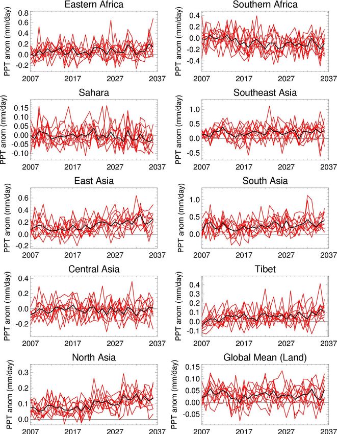
Executive Summary ..................................................................................................................... 3
1. Introduction ............................................................................................................................... 5
2. Aim of the project and background ............................................................................................ 6
3. Data and methodology ............................................................................................................... 6
4. Predictions of changes in precipitation by 2030 ........................................................................10
   4.1. Predicted changes in annual, seasonal and monthly means .................................................10
   4.2. Predicted changes in short-period precipitation extremes ...................................................23
5. Model evaluation ......................................................................................................................29
6. Concluding remarks ..................................................................................................................35
Appendix

Prepared by Anca Brookshaw and Richard Graham, Climate Products, Met Office Hadley Centre

Reviewed by Mike Davey and Anca Brookshaw, Met Office Hadley Centre
Scientific contributors include Holger Pohlmann, Doug Smith, Robin Clark and other Met Office Hadley
Centre scientists
Authorised for issue by Richard Graham, Manager, Climate Products

Date: 25/02/2009

Direct contact: email: anca.brookshaw@metoffice.gov.uk                         Tel 01392 884512

This report was prepared in good faith. Neither the Met Office nor its employees, contractors or
subcontractors, make any warranty, express or implied, or assume any legal liability or responsibility for its
accuracy, completeness, or any party’s use of its contents.

The views and opinions contained in the report do not necessarily state or reflect those of the World Health
Organization and Met Office. The named authors alone are responsible for the views expressed in this
publication.

This report is not edited by the World Health Organization to conform to the requirements of WHO style. The
published material is being distributed without warranty of any kind, either expressed or implied. The
responsibility for the interpretation and use of the material lies with the reader. In no event shall the World
Health Organization be liable for damages arising from its use.

                                                                                                                                               2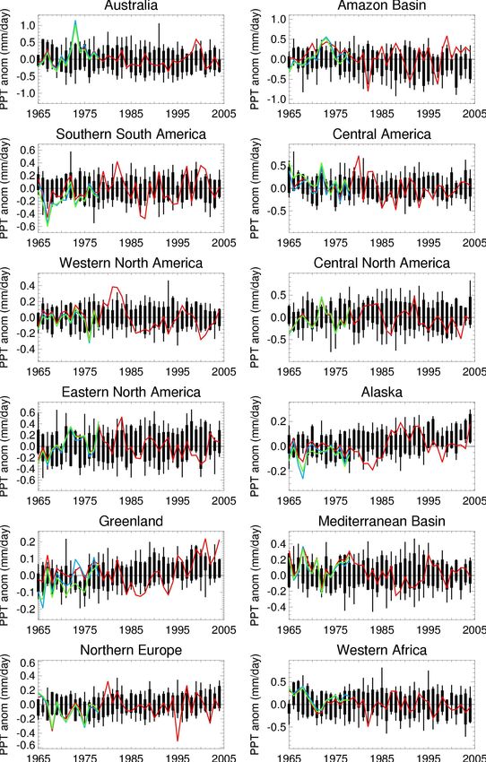
Executive Summary

Changes in climate expected over the next decades, some of which are already
unavoidable, will bring with them the challenge of adapting to the associated impacts. Any
efforts towards adaptation would benefit from the support of credible, robust predictions of
climate changes at regional scales. This study is aiming to inform adaptation strategies in
the sector of water supply and sanitation technologies.

The decadal prediction system (DePreSys) from the Met Office Hadley Centre is used
here as the basis for predictions of changes in precipitation, all around the world, over the
next 20 years. Two time frames during this period are selected for illustration: the 9-year
periods centred on 2020 and 2030 respectively. Predictions are provided for annual,
seasonal and monthly averages, as well as for some large-scale extreme events. The
model predictions are subject to uncertainties, an estimate of which is provided alongside
the prediction maps in the report. Predictions and associated uncertainties will be used,
together with regional information on the status of water supply and sanitation
technologies, to help develop strategies for adaptation.

DePreSys is designed to provide realistic predictions for large-scale changes in climate
over the next few decades, including both natural and man-made influences on the
climate system. Key advantages of the system include:
• it uses a climate model (HadCM3) which is well-established and respected for large
    scale applications,
• it uses observations as initial conditions for the predictions,
• ensembles of predictions provide some estimate of uncertainty due to initial conditions.

Although, arguably, this is the best currently available tool to predict changes in climate
for the near-future, there are caveats to consider when using the predictions:
• in common with other state-of-the-art climate models, a number of key processes for
    local-scale precipitation are poorly – or not at all – represented in the underlying
    model;
• initial-condition uncertainty is not fully sampled; other sources of uncertainty (relating
    to model formulation or future greenhouse-gas emissions) are not investigated;
• the corrections applied to the model output to derive the predictions are relatively
    simple and unlikely to compensate for all modelling errors.

In general, because the science of decadal prediction is at a very early stage, a lot more
fundamental research is needed before meaningful statements of confidence in these
predictions can be made. A rigorous quantitative assessment of their reliability (by
‘predicting’ past cases) is not possible at this stage, but case studies presented in this
report show that plausible predictions of annual-mean precipitation over large-scale areas
are achievable with DePreSys. The value of information on individual regions would be
greatly enhanced by combining it with detailed understanding of the regional meteorology
and of the strengths and limitations of climate models at regional scales.

In the absence of quantitative assessments of confidence in the predictions, consistency
between models has been used to categorise the predicted changes; the robust findings,
according to this criterion, are summarised below.

                                                                                               3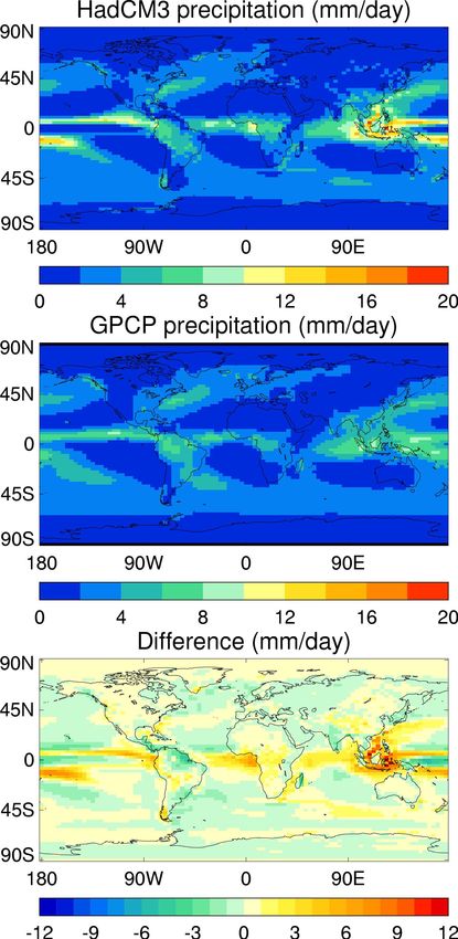
•   Patterns of change predicted for the period around 2020 appear spatially coherent,
       and are mainly large scale. They are broadly similar to the patterns of predictions
       for the period around 2030.

   •   Annual-mean precipitation is predicted to increase in high-latitude areas, in both
       hemispheres, with changes predicted to become apparent by the 2020s;
       precipitation is predicted to decrease in southern Africa, parts of Central America
       and of the Mediterranean basin by the 2030s (more than two thirds of models
       analysed agree).
   •   Additionally, annual-mean precipitation is predicted to decrease over northern
       South America and some parts of Central America, starting by the 2020s and
       continuing at least to the 2030s, and is predicted to increase over South Asia,
       already by the 2020s, persisting or increasing further by the 2030s, as well as over
       parts of central Africa (more than two thirds of HadCM3 models agree, but less
       agreement among other models).
   •   Additionally, annual-mean precipitation is predicted to decrease in coastal regions
       of western North America, starting by the 2020s, and in the Mediterranean region,
       by the 2030s; annual-mean precipitation increases are predicted for some parts of
       the Sahel region of western Africa (all DePreSys predictions agree, but less
       agreement among other models).

It must be emphasised that these are predictions for 9-year averages centred on 2020
and 2030 respectively; uncertainties in variability of individual years around these dates
are large over the whole globe. More generally, even confident predictions by one or
several models remain subject to model error, and thus cannot be guaranteed.

A limited analysis of predicted changes, around 2030, in large-scale extreme events
lasting a few days, reveals uncertainty in the sign of the expected changes, in most parts
of the world. However, some features are supported by 90% of members of the DePreSys
ensemble; these are summarised below.
    • The intensity of wet 5-day large-scale events is predicted to decrease in parts of
       the Middle East, northeastern and southwestern Africa as well as in northeastern
       Brazil and some coastal areas in western North America; areas in eastern Asia and
       parts of the northern extratropics show relatively large risk of increase in intensity
       of such events.
    • The number of dry 10-day periods is predicted to increase over parts of southern
       Africa, over large areas in central and eastern South America, areas of the
       Mediterranean basin and the coastal region of western North America. These
       changes are consistent with the predictions that these areas will be drier in the
       annual mean.

In light of the considerations listed above, the predictions presented here may be
cautiously used to gauge large-scale patterns of change across the globe; they should not
be used for applications which require small-scale details.

                                                                                             4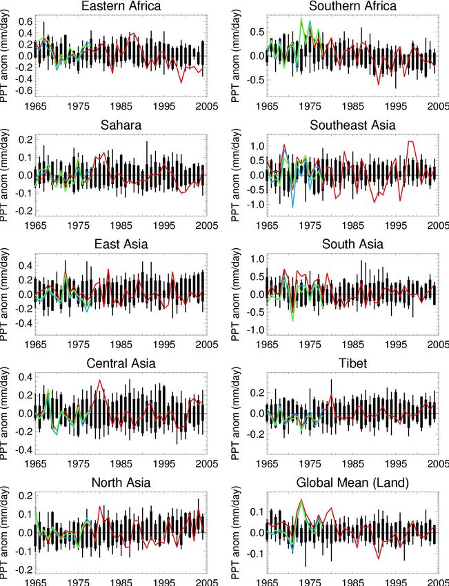
1. Introduction

Climate change will have impacts on many sectors of activity and in all parts of the world;
many such impacts are already being felt. Predictions of expected changes have the
potential to help plan for the future, by informing adaptation strategies.

Causes of changes in climate vary with time into the future – changes due to
anthropogenic influences on the climate system are modulated by, and act alongside,
changes due to natural variability. This is particularly the case in the ‘near’ future (a few
years ahead), when the expected human influences are still relatively small, and their
effect is comparable to that of the natural variability of the system. A variety of climate
prediction systems have been designed to exploit the various sources of predictability.

The Met Office’s decadal prediction system is used in this project to assess changes in
precipitation over the next 30 years. This system is designed to take account of the
current observed global climate state, and as a consequence is expected to give a better
estimate than ‘IPCC-type models’ of the changes expected over relatively short periods in
the future when the influence of climate variability is thought to make a significant
contribution to the expected changes.

Climate predictions inevitably refer to time averages and space averages; prediction of
individual weather events years into the future is not possible. Predictions are presented
here for changes in period means at all locations around the globe; a summary
assessment of changes in precipitation extremes is also included. The model the
predictions are derived from, like most climate models, has coarse resolution, and as a
consequence the results are applicable for large-scale changes. Further analysis, taking
account of local influences on precipitation, would be needed for applications at local
scales. As predictions are inherently uncertain, it is important to assess the associated
uncertainty, especially if decisions are to be based on these predictions; some estimates
are given here, but they are based on limited information (given the scope and extent of
the project).

The report starts by presenting the aim of the study, in section 2; section 3 describes the
data and methodology employed. In the main part of the report, section 4, predictions are
presented both for the changes in mean precipitation and in statistics of extremes. Section
5 looks at evidence on the model’s ability to reproduce observed recent climate; it also
includes a comparison of the predictions presented here, derived from the decadal
prediction system, with some predictions for the same period obtained from other climate
models. The final section presents a few concluding remarks and suggestions for work to
enhance these predictions. It is followed by an appendix including maps of changes in
seasonal- and monthly-mean precipitation, as well as supplementary graphs supporting
the discussion in section 4 (these maps were separated from the main body of the report
to make this easier to read. Many references are made in the text to the maps included in
the appendix, so it is important to regard the appendix as an integral part of the report).

The work has resulted in a global database of predictions to 2030 of annual, seasonal,
monthly and 5-day timescales. This database will be used in parallel work to assess

                                                                                                5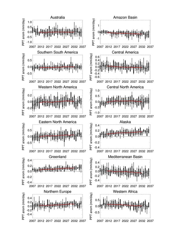
impacts on water and sanitation technologies. Results presented in this report represent
an overview of the information available.

2. Aim of the project and background

The purpose of this study is to provide information about precipitation patterns in the
future and thus support the assessment of the likely impact of climate change on the
viability of technologies currently used (or planned for the near future) to provide water
supply and sanitation consistent with meeting the targets set as part of the Millennium
Development Goals.

If climate change affects the viability of water supply and sanitation technologies, the
consequences may increase the cost of achieving the Millennium Development Goals or
potentially jeopardise the timely achievement of some of the specific targets. This work is
intended to help inform the understanding of the likely impacts of climate change and thus
contribute to the development of evidence-based guidance on which water and sanitation
technologies to promote in different situations. The findings could also be used as a
framework for assessing future development of technologies and their likely cost-
effectiveness and robustness.

Specifically, the study provides predictions of likely changes in global precipitation
patterns expected by 2030 and some estimates of changes at regional level, both in the
mean amount of precipitation and in the intensity of extremes, as well as assessing some
of the uncertainties associated with these predictions. These estimates are based on the
Met Office’s decadal prediction system. Despite the system’s theoretical merits, discussed
in the next section, the estimates presented here have an important limitation: being
derived from a single model, they inevitably ignore any prediction uncertainties due to the
formulation of the model.

As a consequence, this collection of predictions is to be regarded as a generic tool for
‘first order’ assessment of changes at regional scales. Further analysis, including
predictions from other models, would be required for detailed local applications, especially
as far as estimating the true uncertainties in the predictions is concerned.

3. Data and methodology

Modelling framework
The predictions provided as a result of this study are based on the Met Office Hadley
Centre’s decadal prediction system (DePreSys). It is a prediction system designed to
represent changes in the climate over next few decades, when external influences on the
climate system are thought to be comparable in magnitude to the effects of natural
variability. In a departure from the usual techniques of modelling the climate, which only
aim to capture the envelope of natural variability around forced changes, and not to
forecast the phases of the variability, DePreSys predictions are started from observed
conditions which specify the current phase of variability of the climate on interannual (and
decadal, or multi-decadal) timescales. There is evidence to indicate that retrospective
predictions using DePreSys have better skill at reproducing observed decadal averages of
large-scale temperature changes than similar predictions without the information
contained in the initial conditions, at least in the first few years of the prediction (Smith et
                                                                                              6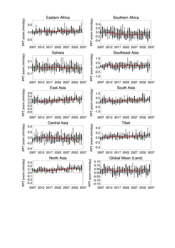
al, 2007). This suggests that even for other variables (including precipitation) and longer-
range predictions – for which the influence of initial conditions is an ongoing research
question – it would be prudent to include observed initial conditions.

DePreSys (Smith et al, 2007), uses Hadley Centre’s climate prediction model HadCM3
(Gordon et al, 2000). This is a coupled ocean-atmosphere general circulation model,
which represents the atmosphere and the oceans, throughout their depth, as latitude-
longitude grids. The atmospheric grid has horizontal resolution of 2.5° in latitude and 3.75°
in longitude and 19 vertical levels; the oceanic grid has horizontal resolution of 1.25° x
1.25° and 20 vertical levels. Variables at each grid point can be regarded as representing
conditions in a grid box: a model grid point on the Earth’s surface represents an area
whose extent depends on the latitude at which it is situated on the globe (e.g. in mid-
latitudes the size of a grid box is approximately 300kmx300km). As a consequence, the
predictions are only meaningful at these or larger scales – any inferences for precise
locations would require supplementary interpretation.

Uncertainty estimation
As part of the prediction system, the model is run in ensemble mode1, with each
ensemble member started from initial conditions created by assimilating observations into
the initial state of both the ocean and the atmosphere, in the form of anomalies from long-
term climatology. The anomaly initialisation approach recognises that the model
climatology is not a perfect representation of the real-world climatology, and is designed
to reduce the impact of the differences (in effect, it uses the model to predict anomalies
relative to its own climate). The forecast used in this study is a 10-member ensemble
started from conditions observed on 10 consecutive days in March 2007. The climatology
of the model is provided by a mean of 4 simulations for 1979 to 2001 made using
HadCM3, which include natural and man-made influences on the climate system, such as
volcanic eruptions and anthropogenically produced greenhouse gases (referred to as
‘forcings’).

Predictions
In this study, changes are estimated in the annual, seasonal (3-month averages) and
monthly means of precipitation and presented as maps and graphs. On the maps
provided, the value indicated in each grid box represents the average of values at the box
in question and the 8 grid boxes surrounding it; these will be referred to as 9-box
averages, centred at the given location. This is done to smooth the grid-scale spatial
variations that can be artefacts of small scale ‘noise’ in the system and thus not
representative of actual variations. Aggregating information over larger areas is necessary
in order to achieve scales at which global climate models can be expected to resolve
regional climate features with reasonable skill. In general, skill of predictions increases
with averaging, both in space and in time. Year-to-year changes over the next 30 years
are presented in this report only for annual means of large-area averages. These
predictions are not intended to offer precise year-to-year sequences, but illustrate typical

1
  An ensemble, in this context, is a set of predictions designed to quantify uncertainties in the outcomes predicted,
given uncertainties in the inputs into the model. For example, DePreSys is an initial-value ensemble which uses ten
different forecasts (‘members’) to estimate the expected range of changes in climate variables; the ensemble members
differ only by their initial conditions. This approach is needed for long-range predictions: small differences in the
initial state of the atmosphere and ocean can amplify to large differences in the outcomes predicted for months or years
into the future.
                                                                                                                      7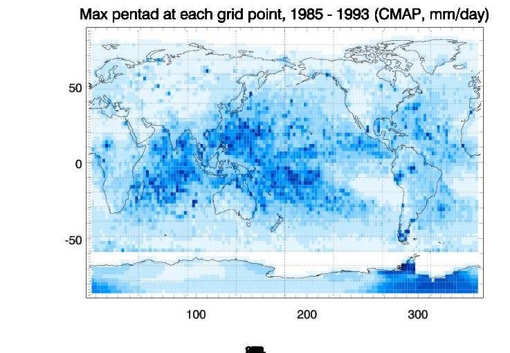
interannual variability. The regions used are those defined by Giorgi and Francisco (2000)
for regional analysis of climate model simulations, and are listed below.

Name                                Acronym           Latitude (°) Longitude (°)
----------------------------------------------------------------------------------------
Australia                           AUS               45S-11S           110E-155E
Amazon Basin                        AMZ               20S-12N           82W-34W
Southern South America SSA                            56S-20S           76W-40W
Central America                     CAM               10N-30N           116W-83W
Western North America               WNA               30N-60N           130W-103W
Central North America               CNA               30N-50N           103W-85W
Eastern North America               ENA               25N-50N           85W-60W
Alaska                              ALA               60N-72N           170W-103W
Greenland                           GRL               50N-85N           103W-10W
Mediterranean Basin                 MED               30N-48N           10W-40E
Northern Europe                     NEU               48N-75N           10W-40E
Western Africa                      WAF               12S-18N           20W-22E
Eastern Africa                      EAF               12S-18N           22E-52E
Southern Africa                     SAF               35S-12S           10W-52E
Sahara                              SAH               18N-30N           20W-65E
Southeast Asia                      SEA               11S-20N           95E-155E
East Asia                           EAS               20N-50N           100E-145E
South Asia                          SAS               5N-30N            65E-100E
Central Asia                        CAS               30N-50N           40E-75E
Tibet                               TIB               30N-50N           75E-100E
North Asia                          NAS               50N-70N           40E-180E

Following their method, only model land grid points from each region are used in the
analysis. A map of these regions and country boundaries is in Figure 1.

Figure 1 Giorgi regions

                                                                                           8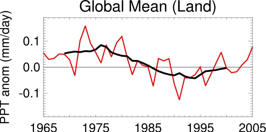
The changes in precipitation (whether in annual, seasonal or monthly means) are
presented as anomalies relative to the climatology for 1979-2001. We make use of both
the model climatology and an observed climatology. Unless specified otherwise, the
‘present day’ climatology refers to the model climatology over the period 1979-2001, and
is estimated as the mean of a 4-member ensemble of HadCM3 predictions with forcings
derived from observations. In most cases the target times for the predictions are 2020 and
2030. To increase the robustness of the results, unless specified otherwise, each of the
predictions is estimated by 9-year averages centred on the target year in question (e.g.,
the predictions for a season of 2020 are obtained as averages of model predictions for the
same season in the 9 years 2016-2024). Although individual years are not predictable
years in advance, due to influences of natural fluctuations from year to year, the 9-year
average is potentially more predictable.

Changes to the statistics of extreme ‘events’ at grid-box scale are estimated from daily
data output by the forecast model. Predictions are based on the same 10-member
ensemble initialised in March 2007. The method used follows that of Clark et al. (2006)
and Clark and Brown (2008). Changes in extreme rainfall statistics are calculated by
comparing DePreSys forecasts for the 9 years 2026-2034 (centred on 2030) with
DePreSys hindcasts (retrospective forecasts) for the 9-year period 1985-1993 (centred on
1989), described below.

Data for model evaluation
A set of hindcasts using DePreSys was created to help assess the skill of the system by
comparison with observations. The hindcasts are 4-member ensembles (started from
consecutive days), with start dates at 3-month intervals, from initial conditions created by
assimilating observations. The external forcings applied to the system are derived from
concentrations of greenhouse gases and sulphate aerosol provided by SRES scenario
B22 (see IPCC, 2007), observed volcanic aerosol decayed from the initial value with one-
year timescale and solar forcing obtained by repeating the previous 11-year solar cycle.
The hindcast dataset covers the period 1979-2001; for each year 4-member hindcast
ensembles are started from March, June, September and December. In addition, two 10-
member hindcasts were initialised 10 years apart, in 1965 and 1975 respectively, and run
for 30 years each, with external forcing similar to those used for the shorter hindcasts –
further discussion on these hindcasts is available in the section on model evaluation.

Data from other climate models is used to set the DePreSys prediction in a wider context
of climate change predictions. The methodology will be fully explained in the section on
model evaluation; in brief, it consists of comparing maps of predicted changes in
precipitation (for 9-year periods centred on 2020 and 2030 respectively), similar to the
maps of changes projected for the end of the century included in the report by the
Intergovernmental Panel on Climate Change (IPCC), on the physical science basis of
climate change (IPCC 2007, Figure SPM.7). Two prediction systems are used for this
comparison. The first is an ensemble formed by perturbing parameters in the physics of
the atmospheric part of HadCM3, with the aim of quantifying uncertainties due to
parametrisations used in one model. This ensemble will be referred to as the QUMP

2
  The choice of scenario is assumed to make little difference to the predicted outcome: differences in global average
temperature predicted under different scenarios have been shown to be small up to around 2030. However, since the
distribution and concentration of aerosols is important for regional predictions of precipitation (and these differ from
scenario to scenario), this is a limiting assumption.
                                                                                                                           9
ensemble (from ‘quantifying uncertainties in model predictions’, the name of the project
which gave rise to it – Murphy et al, 2004). Each of its members is a slightly different
model version from the others, with the differences between models restricted to the
physics of the atmospheric component. The QUMP ensemble is designed to
systematically sample a wide range of process uncertainties. The second is the multi-
model ensemble formed from all the models participating in the IPCC’s 4th assessment,
and will be referred to as the AR4 ensemble. This ensemble samples (in an ad hoc way) a
wider range of uncertainty due to model formulation than the QUMP ensemble
(participating models may have different physics, dynamics and resolution). In practice,
the two types of ensembles give similar ranges of changes in key aspects of large-scale
climate change by the end of the century (for a given emissions scenario). The predictions
available to this study from these two ensembles all use external forcings specified by
SRES scenario A1B.
Observations are used for converting predicted percentage changes into amount changes
and for evaluating the model’s performance in reproducing the observed precipitation
variability from 1979 onwards. For the period since 1979 data from the Global
Precipitation Climatology Project (GPCP, Adler et al. 2003) are used for annual, seasonal
and monthly averages, and data from the CPC Merged Analysis of Precipitation (CMAP,
Xie, P., and P.A. Arkin, 1997) are used for 5-day averages ; for the period prior to the
satellite era data from the Goddard Institute for Space Studies (GISS, Dai et al. 1997) the
Climate Research Unit (CRU, Hulme 1992) and the Variability Analysis of Surface Climate
Observations (VASClimO, Beck et al. 2005) project are used.
4. Predictions of changes in precipitation by 2030
4.1. Predicted changes in annual, seasonal and monthly means
Using data from a 10-member DePreSys ensemble forecast initialised with conditions
observed in March 2007, estimates are generated for the changes in precipitation
amounts expected around 2020 and 2030. Deterministic estimates of the changes in
annual-mean precipitation are calculated as 9-year averages centred on the target year.
At each ‘location’ (grid point) the value plotted is the average of the model output over a
3x3 grid-point array centred on the location in question. Predicted changes are shown
both as percentages (of climatological values) and amounts. Percentage changes are
calculated directly from model data, as (model absolute value - model climatology)/model
climatology. This represents, in ‘model world’, the changes expected as a proportion of
current (1979-2001) values.
As illustrated in Figure 2, the ‘model world’ and the real world climatologies differ to a
certain extent. The differences are largest in the tropics, especially over southeastern
Asia, and they are a rough measure of model error (though it is likely that there is also
uncertainty in the observations). It is clear from these differences that amount and
percentage changes will not both be the same in the modelled and observed ‘worlds’. We
can either assume that the observed anomalies (absolute value – climatology) are well
represented by the model and assume them to be invariant between the model and the
real world – in which case the relative changes, obtained by dividing the anomalies by the
climatological values will differ between model and observations – or assume that the
relative change ((absolute value – climatology)/climatology) is the invariant measure, in
which case the anomalies in the real world must differ from those directly predicted by the
10model. Neither of these assumptions is likely to be entirely defendable without a deeper
understanding of the source and structure of model errors (which is beyond the scope of
this project). We proceed here with the latter assumption, and use the relative changes
derived exclusively from the model as good representations of the relative changes
expected in the real world; to calculate the amount changes expected we multiply the
expected relative change by the observed climatological value at each location.
Figure 2 Annual-mean precipitation climatology for 1979-2001: model (top map), observations (middle map)
and the difference (bottom map), all expressed in mm/day
This procedure removes the mean bias and part of the bias in the variance in the model
predictions. However, it is unlikely to fully correct the model data at most locations;
predictions for areas where the differences between the observed and modeled climate
are large (e.g. southeastern Asia) should be viewed with considerable caution. Also, it
must be emphasised that given the coarse resolution of the model, some important
processes which influence regional precipitation are poorly represented, or missing
11entirely (e.g. strong topographical forcing) – in such areas (e.g. high terrain, not correctly
reflected in the model topography) more detailed analysis of model biases would be
necessary to increase confidence in the predictions.
It is important to take into account both the predicted relative changes and the changes in
amounts. In regions where (at certain times of year, at least) the precipitation amounts are
low, apparently small changes (negligible, in the convention adopted in the plots
presented here) may represent a large proportion of current levels and potentially have a
larger impact than the absolute value of the change might suggest. Conversely, large
percentage changes which in fact reflect small absolute amounts could mislead on the
severity of the expected impacts if not accompanied by the information on changes in
amounts.
The ‘best estimate’ changes in 9-year averages are calculated as means of the 10-
member ensemble. (There are other ways – not presented here – of deriving a best
estimate for predicted changes; the optimal choice would ultimately depend on the
application the predictions are used for.) A 9-year average is regarded as an ‘average’
year around the target date, and as such will not exhibit precisely the same variability as
individual years; however, it is preferred for ‘best estimates’ as it’s likely to be more
predictable than individual years. An example of how 9-year average values compare with
corresponding values for individual years is illustrated in Figure 3, where annual means
(of globally-averaged precipitation anomalies) are plotted on the same scale as 9-year
‘rolling’ means of the same variable. It is evident that the individual values exhibit larger
year-to-year variations than the 9-year means.
Figure 3 Example of differences between changes in individual annual means (red line) and 9-year rolling
averages (black line); see text for explanation
The ‘best estimates’ are accompanied by estimates of the 10%-90% range for predicted
annual-mean precipitation changes. Expected ‘extreme’ values of annual-mean
precipitation, which are highlighted by the 10%-90% range, are deemed of more interest if
calculated for individual years, represented by the model, than for 9-year averages. The
range is delimited by the 10th and 90th percentiles of the set of predictions available at
each grid point for the target period (where the 90 predictions from each of the 10
members and for each of the 9 years around the target date are considered separately.
Years and ensemble members are considered interchangeable within the sample: any
one of them might occur at the target date, so they provide information about the range
and likelihood of possible outcomes according to this model. The ‘best estimate’, although
in most case lying between the ‘limits’ provided by the 10th and 90th percentile grid-point
estimates, is in no direct way related to them. As before, the original grid-point values for
these limits are then averaged over a 9-box area surrounding each location and plotted at
all grid points). It is important to note that, unlike the maps illustrating best-estimate
12changes, the maps of 10th and 90th percentile values do not represent patterns possible in
the future, but simply a collection of individual grid-point percentile values presented on a
map - that is, two neighbouring points on the map may not originate from the same
ensemble member, and thus not be part of the same possible future ‘scenario’.
As a consequence, based on the DePreSys ensemble, in an individual year there is up-to-
10% chance of the expected changes in annual-mean precipitation at each grid point to
be of less than the predicted 10th percentile value and up-to-10% chance of their being
larger than the predicted 90th percentile - and therefore 80% chance of the expected
changes to lie between the two limits. However since, by design, this ensemble only
accounts for part of the uncertainties expected in the predictions, and given that model-
predicted uncertainty bounds have the potential to be different from the uncertainties
expected in the real world (even for prediction systems designed to sample uncertainties
in a more comprehensive way), this interval is itself an estimate.3
Annual means
Figure 4 and Figure 6 map the ‘best estimate’ expected changes, around 2020 and 2030
respectively, in annual mean amounts of precipitation, potentially indicating changes in
the overall availability of water, all around the globe. The precise patterns and anomalies,
although reasonably well smoothed by the spatial-averaging technique, are not to be
counted on to the level of detail of individual grid boxes, because of the (coarse)
resolution of the grid used in the prediction model. Also, the magnitude of the predicted
changes should be considered indicative rather than precise, since only partial corrections
have been made to the variance of the model output. It is recognised that in practice
precise magnitude and location of anomalies are very important, but deriving such level of
detail from coarse-resolution models is, at best, a complex task and it has not been
attempted in this study.
Following the IPCC approach, anomaly values are only plotted on the ‘best estimate’
maps at points where at least 7 (of the total 10) ensemble members agree, in sign, with
the ensemble-mean prediction (the sign agreement is on predictions of 9-year averages).
In addition, a version of the maps is available with the anomaly values plotted only at
points where all ensemble members agree, in sign, with the ensemble-mean prediction (to
highlight the points where there is highest confidence, based on this ensemble prediction
system, in the predicted sign of change) – see Figure A1 in appendix.
3
Results presented in the section on model evaluation, based on a limited comparison, suggest that levels of variability
in annual-mean precipitation changes are similar in DePreSys predictions and observations.
13Figure 4 Changes in annual-mean precipitation (in mm/day, top panel, and as percentage of present-day
climatology, bottom panel) predicted for the 2020s; the anomalies are averages over 9 years centred on the
target date (2016-2024)
14Figure 5 10th and 90th percentiles of predictions of changes in annual-mean precipitation in individual years
around 2020 (estimates based on 9 years centred on the target date; 9 grid-point averages plotted at each
location)
15Figure 6 Changes in precipitation (in mm/day, top panel, and as percentage of present-day climatology, bottom
panel) predicted for the 2030s; the anomalies are averages over 9 years centred on the target date (2026-2034)
16Figure 7 10th and 90th percentiles of predictions of changes in annual-mean precipitation in individual years
around 2030 (estimates based on 9 years centred on the target date; 9 grid-point averages plotted at each
location)
17Broadly speaking, the predictions for the two target periods are similar in sign over land
areas. The expected changes appear to be spatially coherent, over land, and mainly large
scale.
More than 66% of ensemble members are in agreement on the reduction in annual mean
precipitation in northern South America (with all ensemble members predicting such
reduction in northeastern Brazil – Figure A1 in appendix), where these changes would
constitute more than 10% of the current annual precipitation amounts; this reduction is
predicted to exacerbate in time. It is also predicted that parts of southern Africa will
experience a reduction in annual precipitation amounts, while areas in western and
central Africa could see an increase in the total precipitation amounts. India and the area
immediately to the north is predicted to expect an increase in annual precipitation
amounts, which would constitute up to 25% increase relative to current amounts, in many
places. In the northern extratropics the predicted change is towards increase in the annual
mean precipitation, with good agreement between the ensemble members - the increases
by 2030 representing between 5% and 25% of current amounts. The same is true for
much of eastern Asia. Over the central and southern parts of North America the
predictions are less robust, apart from in parts of the western United States where a
decrease in total precipitation amounts is predicted to occur around 2020 and persist
beyond. Little change in amounts is predicted over the Mediterranean basin, northern
Africa and central and southwestern Asia – however, even such small amounts represent
5%-25% decrease on the current climatological amounts in the Arabian peninsula and
parts of the Mediterranean region. The changes predicted over most of Indonesia,
although seemingly sizeable in amounts, represent no more than 5% of the present-day
climatology over most of the area (predictions for this area should be viewed with caution:
here, the differences between modelled and observed climatologies are relatively large –
Figure 2 –, pointing to possibly large model errors). The areas of land with largest
predicted relative (to present day) changes by 2030 are parts of northestern Brazil (more
than 25% reduction in precipitation) and an area to the northwest of the Indian peninsula
(more than 25% increase in precipitation). According to the model used in this study,
these changes are robust, occurring in all 10 ensemble members (see Figure A1). Large
changes are also predicted over the oceans, mostly in the tropics – it is likely that these
changes are due to a change (predicted by the model) in the average position of the
intertropical convergence zone, which modulates the precipitation in the region.
Although at many grid points agreement between the ensemble members on the sign of
predicted changes in 9-year means is good, the range of variability in the predictions for
individual years remains large. The 10%-90% confidence interval estimated according to
the method described above encompasses zero at almost all points on the globe (see
Figure 5 and Figure 7). That means that, based on this ensemble of predictions, at all
these points changes of the opposite sign to that shown as best estimate cannot be ruled
out for individual years (as they are estimated to have at least 10% chance of occurring).
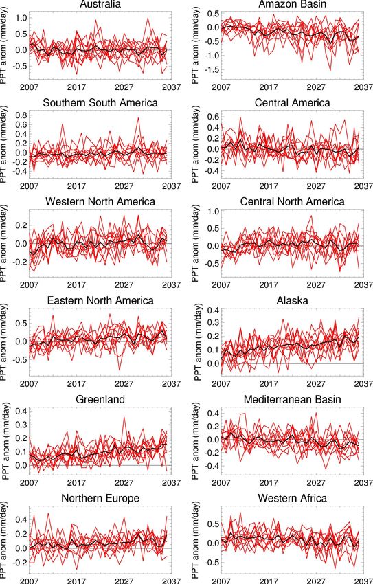
Timeseries illustrating predicted year-to-year variations in annual means for large-area
averages are presented for the Giorgi regions described in the previous section.
Figure 8 illustrates, for each of these regions, the ensemble-mean prediction in black, with
the full range predicted by the ensemble in black vertical lines: the thick section of the
vertical line covers predictions from 8 of the 10 members, with the ends of the thin black
18vertical line representing the ‘extreme’ member prediction at each end of the range for the
given year (note that the identity of the members is not preserved in this plot – for
example, it is not necessarily the same member which predicts the largest change in
precipitation amount for all years). The read line, for each region, illustrates the 9-year
running means centred on the respective year. Individual member predictions for the
Giorgi regions, which illustrate the year-to-year variability as represented by the model,
are also available (Figure A10). From either of these representations it is clear that the
uncertainty in the predictions is large, compared to the ensemble-mean changes.
For some regions, the predictions exhibit trends over the forecast period (noticeable in the
‘smoothed’ timeseries) – e.g., Alaska and East Asia increasing trend, the Amazon basin
and Southern Africa decreasing trend. However, with very few exceptions, anomalies of
opposite sign to that of the long-term trend cannot be ruled out in individual years.
One disadvantage of the Giorgi regions is that they may encompass areas where
predicted changes are of opposite sign. The west-African region is an example: Figure 4
and Figure 6 show predicted increases in the north of the region and decreases in the
south; as a result, the area-average changes throughout the period are small.
1920
Figure 8 Predictions for annual-mean precipitation changes over each Giorgi region: vertical lines – range of
predictions (thick part covers 80% of predictions, thin parts either side extend to cover 10% of remaining
predictions each), horizontal black lines – ensemble-mean predictions for individual years, red lines – ensemble-
mean predictions for 9-year means centred on each year

                                                                                                              21
Seasonal means
A breakdown of the predicted changes by season is illustrated in Figures A2-A5
(appendix), where twelve 3-month seasons are analysed separately. This presentation of
the data is useful for relatively in-depth regional information – e.g. are changes predicted
to happen uniformly through the year, or predominantly in the rainy season, in places
where rain is a seasonal occurrence? Analysis of all possible 3-month seasons is
necessary, since the annual cycle of seasonal precipitation can be very different in
different parts of the world.
It is easily noticeable that the agreement within the prediction ensemble is less
widespread than in the case of the annual averages. Changes in relatively short-period
averages (seasonal and monthly), or over relatively small areas, are likely to be
influenced by unpredictable, fast, variations in atmospheric conditions to a larger extent
than larger-area or longer-term averages; the latter are more likely to change as a result
of slow-varying, and therefore more predictable, oceanic conditions.
Analysing the changes season-by-season highlights regions where changes are predicted
to happen uniformly through the year (at least to the extent of the sign of the change);
northeastern Brazil, western North America and southern Africa to some extent, are all
predicted to experience drying in all seasons. It also becomes apparent that there are
regions where changes of opposite sign are predicted to happen at different times of year,
which cancel out in annual averages – for example eastern Africa (April-June and July-
September in 2030) and the northwestern edges of South America (March-May and
August-October); see Figures A2 and A4 in appendix. These changes may not be
important for overall water availability, but arguably will be important for managing water
resources within the year.
Monthly means
The breakdown of the changes into monthly means adds an extra level of detail, though at
the expense of decrease in agreement within the ensemble (the number of points at which
changes are plotted, where the sign of change predicted by the ensemble mean is the
same as that predicted by more than 66% of individual members, is smaller than that on
the maps of seasonal means, which in turn is smaller than that in the maps of annual
means). For example (see Figure A8 in appendix), information on changes in monthly
means confirms the expectation that the increase in annual-mean precipitation over India
in 2030 is due to increased rainfall predicted for the summer and autumn months, while
very little change is expected in the rest of the year. For some areas, however, this level
of information is not available if a degree of robustness in the predictions similar to that
imposed here (good agreement between individual predictions) is required.
Predictions of changes in monthly means provide a compromise between robust
estimates (long-period averages) and practical need for information on extremes (high-
frequency data, which affect the potential for flooding or drought).
Figures A3, A5, A7, A9 (appendix), which show ranges in seasonal and monthly means in
individual years, bring little supplementary information by comparison with the similar plots
for annual means. There are virtually no land areas where the changes (in the seasonal or
monthly means) are confined to one sign by the 80% range bound by the 10th and 90th
percentiles of the ensemble predictions. Not surprisingly, the range of possible changes to
22be expected in individual years, illustrated by the 10th and 90th percentiles of ensemble
predictions, is larger for monthly and seasonal averages than for annual averages,
especially in place where precipitation is predominantly seasonal or where changes are
expected not to occur uniformly through the year.
4.2. Predicted changes in short-period precipitation extremes
Certain types of water supply and sanitation technologies in wide use are sensitive to
periods of intense rainfall over a few days. For example, water in open wells is prone to
contamination under flood conditions. Potential changes in such extremes cannot be
discerned from the predicted long-period-average changes discussed above. In this
section we investigate predicted changes in extreme rainfall by directly assessing
changes in the intensity of very-wet 5-day periods. The 5-day time span used is
somewhat arbitrary, but has been chosen in order to capture intense rainfall spells long
enough to increase risk of flooding, but short enough to exclude cases where intervening
dry days may allow some natural drainage (thus decreasing the flood risk). We also
examine changes in the frequency of 10-day continuous dry spells, on the assumption
that increases in frequency of such events will have greater impact than a more uniform
lessening of rainfall – even when resulting annual mean changes are similar in both
cases. More extreme events (with potential for more severe impacts), like intense 1-day
precipitation events, or periods of no rain longer than 10 consecutive days, are not
assessed here.
As potential for increased flood risk is likely to be better gauged from predicted changes to
absolute amounts associated with very wet 5-day periods than from percentage changes
(as percentage changes can be large even when amount change are relatively small), we
focus here on predicted absolute changes. It must be emphasised that the predicted
changes are changes to averages over the large geographical areas represented by each
grid box. Thus the extreme events addressed here are essentially ‘large-scale’ extreme
events, and the numerical values cannot be used directly to judge potential increases in
the localised extreme events which will more frequently be the cause of adverse impacts.
Nevertheless it can be assumed that increased intensity of the large-scale extreme events
implies increased intensity of localised events. Downscaling the predictions has been
beyond the scope of this study, but would be useful to obtain information on likely impacts
at local scales.
The predicted changes to large-scale extreme events add illustrative detail to the changes
in annual, seasonal and monthly totals. Because the same prediction model is used, we
can expect the changes to extremes to be broadly consistent with those found for
seasonal and annual periods. However, there is much less potential for validation of
predicted changes to extremes, than predicted monthly, seasonal or annual changes. This
is because there is less observed ‘ground truth’ on daily precipitation climatology, and few
similar prediction studies with other models which might enable a qualitative comparison
of results. Moreover, the 9-year windows used to represent present-day and 2030
conditions may be too short to provide robust climatologies of extreme rainfall.
As an indication of the model’s ability to reproduce 5-day precipitation amounts, Figure 9
illustrates a comparison of observed and predicted total precipitation amounts during the
wettest 5-day period during 1985-1993, at each grid point (as they are averages over the
23area of a grid box, each of these amounts are only indicative of the true local extreme
rainfall). The observed values plotted on the map are from the CMAP dataset described in
section 3; the model values are a mean of 8 ensemble members from DePreSys
hindcasts, (4 started in 1984 and 4 in 1985), the same hindcasts used as baseline for
estimating the changes around 2030.
Figure 9 Amount of rainfall (mm/day) in wettest 5-day period during 1985-1993; top panel - observations,
bottom panel – model
The correspondence is reasonably good, especially over land, with broad-scale similarity
in the patterns, if not always in the magnitude, of the most intense 5-day rainfall events.
The differences are an indication of model biases and of sampling issues, though
uncertainties in the observed data are likely to be important, as well. This comparison
provides some indication that the model can produce ‘events’ with intensity comparable to
observations in approximately the right places. For applications at particular locations,
more detailed comparison would be needed, provided suitable observations were
available.
For the various reasons discussed above, the results presented below must be
considered to represent possible changes to large-scale extreme rainfall events that are
24consistent with the signals for longer-period-average changes presented previously.
Because of the indicative nature of the results, only the 2030 window is addressed.
Procedure for very wet 5-day events
The procedure used follows a two-step approach. Firstly, a reference for the ‘present day’
intensity and frequency of very wet 5-day periods is generated using 8 ensemble
members from hindcasts for the 9-year period centred on 1989 (1985-1993; chosen
because of availability of large enough sample of daily hindcast data). For each ensemble
member, and at each grid box, the entire 9-year sequence is divided into non-overlapping
5-day periods. The 5-day periods are then ranked in decreasing order of magnitude, such
that rank 1 corresponds to the wettest 5-day period in the sequence. The 5-day rainfall
totals corresponding to matching ranks in the 8 ensemble members are then averaged,
providing an ensemble-mean reference for the wettest, second wettest etc, 5-day periods
under current (1989) climatology.
Secondly, a similar ranking process is conducted for 5-day rainfall totals in each of the 10
ensemble members in the DePreSys prediction, using the 9-year sequences for 2026-
2034. For each ensemble member differences are calculated between the predicted 5-day
totals and the totals of the matching rank in current (model) climatology calculated in the
first step, to remove the mean model bias. Thus a sample of 10 potential changes to the
intensity of the wettest, second wettest etc. 5-day periods is obtained. The sample
provides a measure of the uncertainty in the predicted changes and is used to estimate
the 10th and 90th percentile of changes (for brevity, referred to as the upper and lower
estimates). These uncertainty estimates are the best objective measures available with
the current method, but for the reasons stated above are almost certainly underestimates
of the true uncertainty range.
Results for very wet 5-day events
Lower and upper estimates of absolute changes in the wettest (rank 1) and 9th wettest
(rank 9) 5-day periods, representative for 2030, are provided in Figure 10. The rank-1
event occurs once in the 9-year sample and in simple terms has return period of 9 years.
Rank -9 or wetter events occur 9 times in 9 years, and thus have a return period of 1 year.
There is consistency in the changes for rank 1 and rank 9, as well as for less extreme
ranks (not shown). The similarity in sign of change for neighbouring ranks indicates that
results are not over-sensitive to small changes in the rank, suggesting that the distribution
for a given rank is less likely to be the result of ‘random’ extremes than that of organised
large-scale changes captured by the ensemble, and adding confidence to the robustness
of the analysis. It is also notable that, in most regions, the sign of the change differs
between the lower and the upper estimate, indicating that there is relatively large spread
in the ensemble. Exceptions are small areas in northeastern South America and the
Arabian peninsula, where the 80% range appears to confine the predicted changes to a
range between no change and reduction in the amount received during the wettest
events, and parts of central Africa, where changes (in 80% of the predictions) range
between no change and small increase (of up to 30mm in 5 days at grid-box scale) in the
wettest events. Predicted changes are small in less extreme wet ranks (of which only rank
9 is shown here), with the range of changes, in most places, predicted to be between
decrease and increase of up-to 15mm/pentad (at grid-box scale).
25Figure 10 Predicted 2030 change in total rainfall associated with (a) the rank 9 and (b) the rank 1 wet 5-day
periods, in mm/pentad. Left/right hand plots show the 10th/90th percentile changes (calculated as average of
predictions from 1st and 2nd/9th and 10th member) respectively, at each grid point; 8 of the 10 member-
predictions fall within the range between the lower and upper estimate. Changes are based on differences in 9-
year samples centred on 2030 and 1989 (for ‘present day’ climate). See text for further details.
For the assessment of the impact of changes in wet extremes on the vulnerability of water
supply and sanitation technologies, an estimate of the most likely predicted changes at
each location is required. It is recognised that the most important threat for many of the
technologies addressed here is likely to be the increase of the potential for flooding. To
the extent to which an increase (of any severity) in amounts of precipitation received in 5
consecutive days increases the risk of flooding (and assuming that such increases will be
reflected in values of grid-box averages), the proportion of ensemble members predicting
increases in 5-day amounts is provided for this purpose (and illustrated in Figure 11). This
is intended as an indication of the confidence in the predictions of increases, without detail
about the severity of the increase – bounds on the magnitude of the potential changes are
provided by the 10th and 90th percentile estimates.
These maps of grid-point values clearly indicate whether the more likely outcome
predicted by the DePreSys ensemble for each location is of reduction (where fewer
members predict increases than decreases) or of increase in 5-day precipitation amounts.
For top-rank events the predictions show relatively few places with, ‘confident’ changes
(the most notable being small parts of northeastern Africa and the Arabian peninsula); for
rank-9 events the ‘pattern’ highlights larger areas where the predictions indicate low risk
of increase in wet-event intensity (e.g. northeastern Africa, the Middle East and the
26Mediterranean basin, parts of northwestern Africa, western parts of southern Africa,
eastern Australia and northeastern Brazil). Areas where the ensemble predicts sizeable
risk of increase in intensity over land are mostly in the northern hemisphere, away from
the tropics.
Figure 11 Uncertainty in predicted increases in 5-day precipitation amounts: each colour represents a number
of ensemble members indicating increases, white covers the places where 4, 5, or 6 members predict increases.
Further analysis for a region of western Africa, centred at 0˚E, 10˚N, and a region of
southern Africa, centred at 20˚E, 25˚S, is presented in Figure 12 as example to highlight
consistency of changes through the top ranks of the 9-year sequences. The changes in
totals over 5-day wet events around 2030 are shown for the top-100-ranking events. Here,
changes in the median, 10th and 90th percentiles are calculated using data from all 10
ensembles from a 3x3 grid array centred on the location (90 samples).
Figure 12 Predicted changes in 2030 rainfall totals associated with the top-100-ranking wet 5-day events,
extracted for a grid box location: 0˚E, 10˚N (in West Africa), left panel, and 20˚E, 25˚S (southern Africa), right
panel. The median, 10th and 90th percentile changes are shown. Changes are based on differences between 9-year
samples centred on 2030 and 1989 (for ‘present day’ climate). See text for further details.
For the location in western Africa the 10th-90th percentile range covers changes from
decreases of around 15mm/pentad to increases of around 10mm/pentad (for the top few
ranks). Changes predicted for less extreme ranks are smaller, but their ranges include
zero. The relatively smooth nature of the dependency on rank suggests that results are
not unduly sensitive to the precise rank selected (i.e. similar results are obtained for
neighbouring ranks), and this adds confidence in the robustness of the analysis.
27You can also read