Probabilistic Models for Inference about Identity
←
→
Page content transcription
If your browser does not render page correctly, please read the page content below
144                                    IEEE TRANSACTIONS ON PATTERN ANALYSIS AND MACHINE INTELLIGENCE,                        VOL. 34,   NO. 1,   JANUARY 2012

Probabilistic Models for Inference about Identity
             Peng Li, Member, IEEE, Yun Fu, Member, IEEE, Umar Mohammed, Member, IEEE,
                  James H. Elder, Member, IEEE, and Simon J.D. Prince, Member, IEEE

       Abstract—Many face recognition algorithms use “distance-based” methods: Feature vectors are extracted from each face and
       distances in feature space are compared to determine matches. In this paper, we argue for a fundamentally different approach. We
       consider each image as having been generated from several underlying causes, some of which are due to identity (latent identity
       variables, or LIVs) and some of which are not. In recognition, we evaluate the probability that two faces have the same underlying
       identity cause. We make these ideas concrete by developing a series of novel generative models which incorporate both within-
       individual and between-individual variation. We consider both the linear case, where signal and noise are represented by a subspace,
       and the nonlinear case, where an arbitrary face manifold can be described and noise is position-dependent. We also develop a “tied”
       version of the algorithm that allows explicit comparison of faces across quite different viewing conditions. We demonstrate that our
       model produces results that are comparable to or better than the state of the art for both frontal face recognition and face recognition
       under varying pose.

       Index Terms—Computing methodologies, pattern recognition, applications, face and gesture recognition.

                                                                                 Ç

1     INTRODUCTION

G    ENERATIVE probabilistic formulations have proven suc-
     cessful in many areas of computer vision including
object recognition [12], image segmentation [36], and
                                                                                     distance from the probe feature vector. In face verification,
                                                                                     two face images are ascribed to the same individual if the
                                                                                     distance in feature space between them is less than some
tracking [3]. These algorithms assume that the measure-                              threshold. The logic of this approach is that for a judicious
ments are indirectly created from a set of underlying                                choice of feature space, the signal-to-noise ratio will be
variables in noisy conditions. Vision problems are formu-                            improved relative to that in the original space.
lated as inverting this process: We attempt to estimate the                             Within the class of distance-based methods, the domi-
variables from the measurements. This is not different from                          nant paradigm is the “appearance-based” approach, which
nonprobabilistic approaches, but Bayesian generative for-                            uses weighted sums of pixel values as features for the
mulations have three desirable characteristics. First, they                          recognition decision. Turk and Pentland [38] transformed
encourage careful modeling of the measurement noise.                                 the image data to a feature space based on the principal
Second, they allow us to ignore variables that we are not                            components of the pixel covariance. Other work has
interested in by marginalizing over them. Third, they                                variously investigated using different linear weighted pixel
provide a coherent way to compare models of different                                sums, [1], [2], [17], nonlinear techniques [44], and different
sizes using Bayesian model comparison. In this paper, we                             distance measures [32].
describe a probabilistic approach to face recognition that                              A notable subcategory of these methods consists of
exploits all of these characteristics.                                               approaches based on linear discriminant analysis (LDA).
                                                                                     The Fisherfaces algorithm [2] projected face data to a space
1.1 Distance-Based Face Recognition                                                  where the ratio of between-individual variation to within-
Most contemporary face recognition methods are based on                              individual variation was maximized. Fisherfaces is limited
the distance-based approach (see Fig. 1). A low-dimensional                          to directions in which at least some within-individual
feature vector is extracted from each face image. The                                variance has been observed (the small-sample problem).
distances between these vectors are used to identify faces of                        The null-space LDA approach [8] exploited the signal in the
the same person. For example, in closed set identification                           remaining subspace. The Dual-Space LDA approach [39]
we choose the gallery feature vector with minimum                                    combined these two approaches.
                                                                                        These models perform excellently for frontal face
                                                                                     recognition (e.g., see [39]). However, they perform poorly
. P. Li, Y. Fu, U. Mohammed and S.J.D. Prince are with the Department of
  Computer Science, University College London, Gower Street, London
                                                                                     when the probe face is viewed with a very different pose,
  WC1E 6BT, United Kingdom.                                                          expression, or illumination from the corresponding gallery
  E-mail: {p.li, y.fu, u.mohammed, s.prince}@cs.ucl.ac.uk.                           image [45]. Distance-based methods fail because the
. J. Elder is with the Center for Vision Research, York University, Room             extracted feature vector changes with these variables,
  0003G, Computer Science Building, 4700 Keele Street, North York,
  Ontario M3J 1P3, Canada. E-mail: jelder@yorku.ca.                                  making the measured distances between vectors unreliable.
Manuscript received 14 May 2010; revised 21 Dec. 2010; accepted 3 Mar.
                                                                                     Indeed, the variation attributable to these factors may dwarf
2011; published online 13 May 2011.                                                  the variation due to differences in identity, rendering the
Recommended for acceptance by T. Jebara.                                             nearest-neighbor decision meaningless. Even LDA-based
For information on obtaining reprints of this article, please send e-mail to:        approaches such as [2], [39] fail as the signal lies in part of
tpami@computer.org, and reference IEEECS Log Number
TPAMI-2010-05-0378.                                                                  the subspace where the noise is also great and is hence
Digital Object Identifier no. 10.1109/TPAMI.2011.104.                                down-weighted or discarded.
                                               0162-8828/12/$31.00 ß 2012 IEEE       Published by the IEEE Computer Society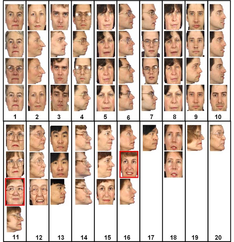
LI ET AL.: PROBABILISTIC MODELS FOR INFERENCE ABOUT IDENTITY                                                                               145

                                                                              They modeled distributions of “within-individual” and
                                                                              “between-individual” differences. For two new images, they
                                                                              find the posterior probability that the difference belongs to
                                                                              each. This is well suited to face verification, but does not
                                                                              provide a posterior over possible matches for other tasks.
                                                                              Moreover, performance in uncontrolled conditions is poor
                                                                              [27]. There is no obvious way to remedy these problems.
                                                                                 Recently, probabilistic recognition algorithms have been
                                                                              proposed which can address all the above tasks [19], [35],
Fig. 1. Conventional distance-based approach. Observed probe xp and           [34]. The key idea is to construct a model describing how
gallery x1...3 images are deterministically transformed from pixel space      the data were generated from identity. Prince et al. [34]
(left) to a lower dimensional feature space (right). Distance in feature
space between the probe image f p and each of the gallery images f 1...3      developed a probabilistic “tied factor analysis” model for
is calculated (arrows). The probe vector f p is associated with the nearest   face recognition. This was specialized to the case of large
neighbor gallery vector (here, f 2 ).                                         pose changes and is a special case of one of the models
                                                                              presented in this paper. Ioffe [19] presented a probabilistic
   Many other approaches have been proposed to cope with                      LDA model for face recognition that is also closely related
variable pose and illumination. Important categories in-                      to one of the models presented in this paper.
clude algorithms which 1) require more than one input                            In this paper, we develop a model in which identity is
image of each face [14], 2) create a 3D model from the 2D                     represented as a hidden variable in a generative description
image and estimate pose and lighting explicitly [4], [5], and                 of the image data. Any remaining variation that is not
3) learn a statistical relation between faces viewed under                    attributed to identity is described as noise. The model is
different conditions [16], [27], [34].                                        learned with the expectation-maximization (EM) algorithm
1.2 Probabilistic Face Recognition                                            [9] and face recognition is framed as a model comparison
                                                                              task. An earlier version of this work was published in [35].
The aforementioned distance-based models provide a hard
                                                                              Code is available via http://pvl.cs.ucl.ac.uk.
matching decision—however, it would be better to assign a
                                                                                 In Section 2, we introduce a probabilistic framework to
posterior probability to each explanation of the data. In a
                                                                              solve face recognition problems. In Section 3, we introduce
practical system (e.g., access control), we could defer the
                                                                              a probabilistic version of Fisherfaces [2], which we term
final decision and collect more data if the uncertainty is too
                                                                              probabilistic LDA (or PLDA). We show that this approach
great. Moreover, a probabilistic solution means that we can
                                                                              sidesteps the small sample problem and produces good
easily combine information from different measurement
                                                                              results for frontal faces. In Section 4, we introduce a
modalities and apply priors over the possible matching
                                                                              nonlinear generalization of this approach. In Section 5, we
configurations.
                                                                              introduce “Tied PLDA,” which allows us to compare faces
    Generative probabilistic approaches have yielded con-
                                                                              captured in very different poses. In Section 7, we discuss the
siderable progress in the closely related problem of object
                                                                              relationship between these models and other work.
recognition (e.g., [12]). Nonetheless, there have been few
attempts to construct probabilistic algorithms for face
recognition. One of the reasons for the paucity of probabil-                  2    GENERATIVE MODELS FOR FACE DATA
istic approaches is the diversity of tasks in face recognition.               Our approach is founded on the following four premises.
These include:
                                                                                  1.   Faces images depend on several interacting factors:
   1.   Closed set recognition: Choose one of N gallery                                These include the person’s identity (signal) and the
        faces that matches a probe face.                                               pose, illumination, etc. (nuisance variables).
   2. Open set recognition: Choose one of N gallery faces                         2.   Image generation is noisy: Even in matching
        that matches a probe or identify that there is no                              conditions, images of the same person differ. This
        match.                                                                         remaining variation comprises unmodeled factors
   3. Verification: Given two face images, indicate                                    and sensor noise.
        whether they belong to the same person or not.                            3.   Identity cannot be known exactly: Since generation
   4. Clustering: Given N faces, find how many different                               is noisy, there will always be uncertainty on any
        people are present and which person is in which                                estimate of identity, regardless of how we form this
        image.                                                                         estimate.
   Until recently, recognition algorithms could not provide                       4.   Recognition tasks do not require identity esti-
posterior probabilities over different hypotheses for all of                           mates: In face recognition, we can ask whether two
these tasks. Liu and Wechsler [26] described a probabilistic                           faces have the same identity, regardless of what this
method in which they model the data for each individual                                identity is.
(after projection to a subspace) as a Gaussian with identical
and diagonal variance. However, this method is only                           2.1 Latent Identity Variables
suitable for closed set recognition and is not a full                         At the core of our approach is the notion that there exists a
probabilistic model as it only describes the data after                       multidimensional variable h that represents the identity of
projection. The scheme of Moghaddam et al. [28] considered                    the individual. We term this a latent identity variable (LIV) and
pixel-wise difference between probe and gallery images.                       the space that it resides in identity space. Latent identity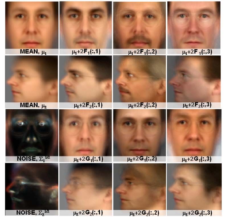
146                                    IEEE TRANSACTIONS ON PATTERN ANALYSIS AND MACHINE INTELLIGENCE,                  VOL. 34,    NO. 1,     JANUARY 2012

Fig. 2. Latent Identity Variable approach. Observed face data vectors x
(left) are generated from the underlying identity space h (right). The
model, x ¼ fðhÞ þ , explains the face data x as generated by a
deterministic transformation fðÞ of the identity variable h followed by the
addition of a stochastic noise term . In this case, the faces x2 and xp are
deemed to match as they were generated from the same underlying
identity variable h2 .
                                                                               Fig. 3. Inference by comparing data likelihood under different models.
                                                                               Each model represents a different relationship between the LIVs h and
variables have this key property: If two variables have                        observations x. (a) Closed set identification with gallery of two faces. In
identical values, they describe the same individual. If two                    Model M1 , the probe xp matches gallery face x1 . In model M2 , the
                                                                               probe xp matches x2 . (b) Open set identification. We add the possibility
variables differ, they describe different people. Crucially, the               M0 that the probe face xp matches neither gallery face x1 nor x2 .
identity variable is constant for an individual, regardless of                 Verification (c) and face clustering (d) can also be expressed as model
pose, illumination, or any other factors that effect the image.                comparison. Note that there is also a noise variable w associated with
                                                                               each datum x which is not shown.
   We never observe identity variables directly, but we
consider the observed faces to have been generated from the
latent identity variable by a noisy process (see Fig. 2). Our                     Fig. 3a shows the model construction for closed set
goal is not necessarily to describe the true generative                        identification. We are given a probe face xp and the
process, but to obtain a model that describes the image data,                  N gallery faces (here, N ¼ 2), each representing a different
within which we can obtain accurate predictions and valid                      person, x1...N . In model Mn the nth gallery face is forced to
uncertainty estimates. In this paper, we consider models of                    share its latent identity variable hn with the probe indicating
the form                                                                       that these faces belong to the same person. Fig. 3c shows the
                                                                               models for face verification. Here, Model M0 represents the
                       xij ¼ fðhi ; wij ; Þ þ ij ;                    ð1Þ    case where the two faces do not match (each image has a
where xij is the vectorized data from the jth image of the                     separate identity). Model M1 represents the case where they
ith person. The term hi is the LIV and is constant for every                   do match (they share an identity). In fact, all four
image of that person (i.e., it is not indexed by j). The term                  recognition tasks from Section 1.2 can be expressed in terms
wij is another latent variable representing the viewing                        of model comparison: For open set identification (Fig. 3b),
conditions (pose, illumination, expression, etc.) for the                      we start with the closed set case and add a model M0
jth image of the ith person. The term ij is an axis oriented                  representing the situation where the probe has its own
Gaussian noise term and is used to explain any remaining                       unique identity. In face clustering (Fig. 3d), we are given
variation. The term  is a vector of model parameters which                    N faces and there may be N different people (N identity
are learned during a training phase and remain constant                        variables), just one person (1 identity variable), or anything
during recognition.                                                            in between. In this paper, we concentrate on closed set
   Assuming that we know the model parameters, , how                          identification, verification, and clustering.
can we then identify if a gallery and probe face match? In                        We combine the likelihoods of these models with suitable
the next two sections, we consider two alternative strategies                  priors P rðMÞ (always uniform in this paper) and find a
based on 1) evaluating the joint probability of probe and                      posterior probability for the match using Bayes’ rule.
gallery images and 2) forming class-conditional predictive                     However, the question remains as to how to calculate the
distributions.                                                                 model likelihoods. Noise in the generation process means
2.2 Recognition: Joint Perspective                                             that we can never exactly know either the identity variables h
                                                                               or the noise variables w in these models. Hence, we
Our framework infers whether two observed images x1 and
                                                                               marginalize (integrate out) these variables:
x2 were generated from the same identity variable h and
hence belong to the same individual. Unfortunately, this                                                             Y
                                                                                                                     N
presents a problem: The data x was generated in noisy                                         P rðx1...N;p jM0 Þ ¼         P rðxn ÞP rðxp Þ;            ð2Þ
conditions, so we can never be certain of the underlying                                                             n¼1
value of h or w. To resolve this, we consider all possible
values of h and w.                                                                                                Y
                                                                                                                  N
   More formally, the recognition process compares the                                  P rðx1...N;p jMm Þ ¼               P rðxn ÞP rðxp ; xm Þ;       ð3Þ
likelihood of the data under different models M. Each                                                          n¼1;n6¼m
model assigns identity variables h to explain the observed
faces x in a different way. If the current model ascribes two                  where
face images to belong to the same person, then they will                                                  ZZ
have the same identity variable. If not, then they will each                                 P rðxn Þ ¼        P rðxn ; hn ; wn Þdhn dwn ;              ð4Þ
have their own identity variables.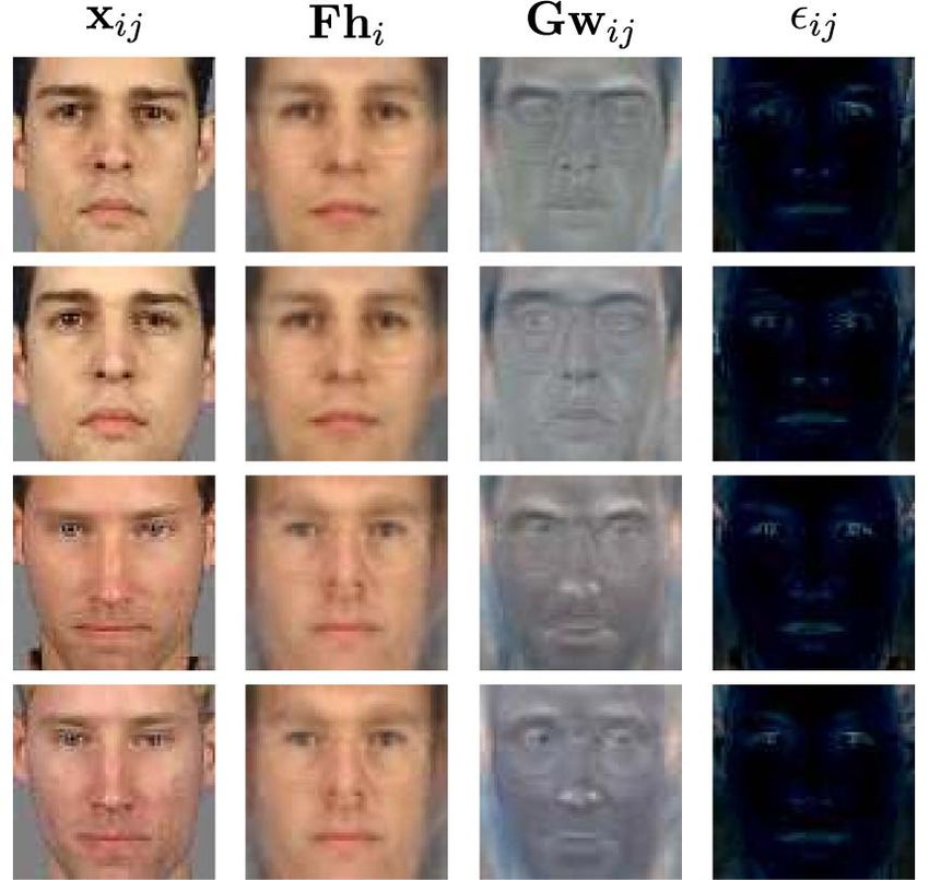
LI ET AL.: PROBABILISTIC MODELS FOR INFERENCE ABOUT IDENTITY                                                                                  147
                            ZZ
               P rðxp Þ ¼        P rðxp ; hp ; wp Þdhp dwp ;        ð5Þ

                      ZZZ
    P rðxp ; xm Þ ¼         P rðxp ; xm ; hm ; wp ; wm Þdhm dwp dwm :

                                                                    ð6Þ
   An important aspect of this formulation is that the final
likelihood expression does not explicitly depend on the latent
identity variables h. This makes it valid to compare models
with different numbers of latent identity variables. For
example, in face verification we compare a model with two                 Fig. 4. PLDA Model. (A) Graphical model relating data x to identities h,
underlying latent variables (no match) to one (match). This is            noise variables w, and parameters  ¼ f; F; G; g. (B) Predictive
                                                                          distribution for subspace model with one identity factor F (dotted line)
an example of Bayesian model selection in which we compare
                                                                          and one noise factor G (not shown). The gray region represents
the evidence for the different explanations of the data.                  associated Gaussian face manifold. New gallery images (red and green
                                                                          dots) induce Gaussian predictive distributions (red and green ellipses).
2.3 Recognition: Class Conditional Perspective
In the previous treatment, we evaluate the joint likelihood               multidimensional Gaussians. It seeks directions in space
of the probe and gallery images under different models ((2)               that have maximum discriminability and are hence most
and (3)). An alternative perspective is to consider the                   suitable for supporting class recognition. We refer to our
predictive distribution for the probe image xp induced by                 version of this algorithm as probabilistic linear discriminant
the matching gallery data xg in each of the models. To make               analysis. The relationship between PLDA and standard
face recognition decisions, we evaluate the likelihood of the             LDA is similar to that between factor analysis and principal
probe image under each of these class conditional density                 components analysis.
functions and combine with priors. Now we write                              We assume that the training data consist of J images
                                                                          each of I individuals. We denote the jth image of the
          P rðx1...N;p jM0 Þ ¼ P rðxp jx1...N ; M0 ÞP rðx1...N Þ          ith individual by xij . We model the data generation as
                                          Y
                                          N                         ð7Þ
                             ¼ P rðxp Þ         P rðxn Þ;                                    xij ¼  þ Fhi þ Gwij þ ij ;                     ð9Þ
                                          n¼1
                                                                          where  is the mean of the data, F is a factor matrix with the
                                                                          basis vectors of the between individual subspace in its
         P rðx1...N;p jMm Þ ¼ P rðxp jx1...N ; Mm ÞP rðx1...N Þ
                                                                          columns, and hi is the latent identity variable that is
                                                Y
                                                N                   ð8Þ   constant for all images xi1 . . . xiJ of person i. Just as the
                             ¼ P rðxp jxm Þ           P rðxn Þ;
                                                n¼1
                                                                          matrix F contains a matrix determining the between-
                                                                          individual subspace, the matrix G contains a basis for the
where P rðxp jxn Þ is found by taking the conditional of (6).             within-individual subspace. The term wij represents the
This approach is closely related to object recognition:                   position in this subspace. The term ij is a stochastic noise
Generative models such as [12] create a separate probability              term, with diagonal covariance .
density for each class. However, in object recognition there                 The term  þ Fhi is the signal and accounts for between-
are usually numerous training examples of each class (e.g.,               individual variance. For a given individual, this term is
cars). For face recognition, we often only have a single                  constant. The term Gwij þ ij consists of the noise or
example of each class (individual). Hence, face recognition               within-individual variance. It explains why two images of
models necessarily deal with the situation of “one shot”                  the same individual do not look identical.
learning [23].                                                               More formally, we can describe the model in (9) in terms
                                                                          of conditional probabilities
2.4 Tractability of Integrals
We are assuming that the integrals in (4)-(6) can be computed.                      P rðxij jhi ; wij ; Þ ¼ Gx ½ þ Fhi þ Gwij ; ;        ð10Þ
This is true for all models in this paper. When they cannot be
computed, one approach is to approximate the distributions                                         P rðhi Þ ¼ Gh ½0; I;                     ð11Þ
over the hidden variables h and/or w by point estimates h    ^
and w.
     ^ The choice of the joint or class-conditional methods                                       P rðwij Þ ¼ Gw ½0; I;                     ð12Þ
now becomes important: In the joint method, the point
estimate of the identity will be based on both the gallery and            where Ga ½b; C denotes a Gaussian in a with mean b and
probe images, whereas in the class-conditional method, the                covariance C. In (11) and (12), we have defined simple
identity will be based on the gallery alone.                              priors on the latent variables hi and wij . The relationship
                                                                          between the variables is indicated in Fig. 4A. It is important
                                                                          to note that (10), (11), and (12) implicitly define the joint
3     MODEL 1: PROBABILISTIC LDA                                          probability distribution required for (4)-(6). The Gaussian
To make these ideas concrete, we investigate a probabil-                  forms for this model have been chosen because they provide
istic model that is closely related to LDA. LDA is a                      clean closed form solutions to these integrals, rather than
technique that models intraclass and interclass variance as               because they represent the true generative process.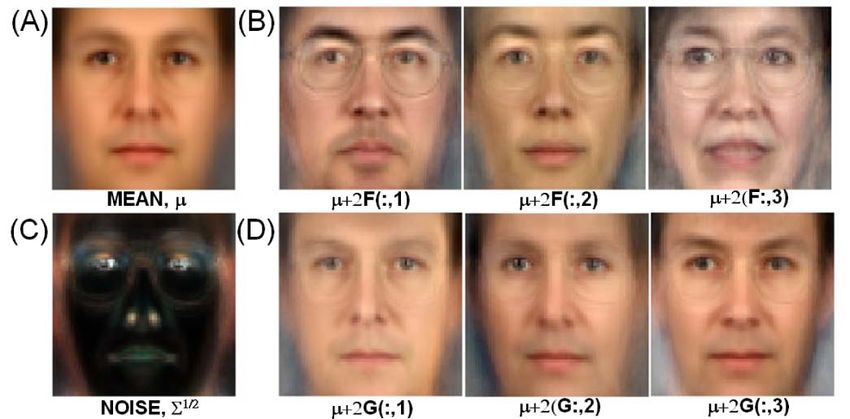
148                                 IEEE TRANSACTIONS ON PATTERN ANALYSIS AND MACHINE INTELLIGENCE,                VOL. 34,   NO. 1,   JANUARY 2012

Fig. 5. PLDA Model. (A) Mean face. (B) Three directions in between-
individual subspace. Each image looks like a different person. (C) Per-
pixel noise covariance. (D) Three directions in within-individual sub-
space. Each image looks like the same person under minor pose and
lighting changes.

3.1 Learning
In the learning stage, we aim to learn the parameters  ¼                 Fig. 6. PLDA. The first column shows the original images xij . These are
f; F; G; g given data xij . It would be easy to estimate these          broken down into a signal subspace component Fhi which is the same
parameters if we knew the hidden identity variables hi and                for each identity, a noise subspace component Gwij , and a per pixel
hidden noise variables wij . Likewise, it would be easy to                noise ij .
infer the identity variables hi and noise variables wij if we                                P rðx0 jyÞ ¼ Gx0 ½0 þ Ay; 0 ;                  ð15Þ
knew the parameters . This type of “chicken and egg”
problem is well suited to the EM algorithm [9]. Details of
this process are given in Appendix A, which can be found                                            P rðyÞ ¼ Gy ½0; I;                        ð16Þ
in the Computer Society Digital Library at http://doi.ieee                where
computersociety.org/10.1109/TPAMI.2011.104.                                                          2                       3
   Fig. 5 shows the results of 10 iterations of learning from                                               0     ...    0
the first 195 individuals from the XM2VTS database with                                             6 0           ...    07
                                                                                               0 ¼ 6
                                                                                                    4 ...    ..    ..     .. 7:                ð17Þ
minimal preprocessing. We show several positions in the                                                       .       .    .5
between-individual subspace (samples where h varies but                                                  0   0     ...
w is constant) and these look like different people. We also
show positions in the within-individual subspace (samples                 This now has the form of a factor analyzer. From (14), it is
where h is constant and w varies). These look like the same               easy to see that the first two moments of the distribution of
person under slightly different illuminations and poses.                  the compound vector x0 are given by
   Fig. 6 shows a visualization of the model for four faces.
In each case, we decompose the image into signal Fhi and                                          E ½x0  ¼ 0 ;
noise components Gwij and ij using the final MAP                              E½ðx0  0 Þðx0  0 ÞT  ¼ E½ðAy þ 0 ÞðAy þ 0 ÞT            ð18Þ
estimate of the hidden variables from the E-Step in training.                                                      T      0
                                                                                                         ¼ AA þ  ;
3.2 Recognition with Joint Method
                                                                          and it can be shown that when we marginalize over the
In recognition, we must evaluate the integrals in (4)-(6). The
general problem is to evaluate the likelihood that N images               hidden variable y, the form of the resulting distribution is
x1...N share the same identity variable, h, regardless of the             Gaussian with these moments:
noise variables w1 . . . wN . Our approach is to rewrite the
                                                                                      P rðx1...N Þ ¼ P rðx0 Þ ¼ Gx0 ½0 ; AAT þ 0 :          ð19Þ
equations in the form of a factor analyzer and use a
standard result for the integral. To this end, we combine the             3.3 Recognition with Predictive Distribution
generative equations for all N images:
                                                                          Instead of calculating the expressions in (2)-(6), we could
                                            2      3
 2      3 2 3 2                            3 h       2 3                  equivalently have performed this experiment by calculating
     x1             F G 0 ... 0 6                 7    1
 6 x2 7 6  7 6 F 0 G . . . 0 7 6 1 7 6  2 7  w                          the predictive distributions P rðxp jx1 Þ . . . P rðxp jxn Þ. We then
 6      7 6 7                               6      7 6 7                  assess the likelihood of the probe image under each of these
 6 .. 7 ¼ 6 .. 7 þ 6  .    ..  .. . .    . 76 w2 7 þ 6 .. 7;
 4 . 5 4 . 5 4 ..           .   .     . .. 56   .. 7 4 . 5                distributions.
                                            4 . 5
    xN              F 0 0 ... G                       N                    The predictive distributions can be calculated by taking
                                              wN
                                                                          the joint distribution in (19) and finding the conditional
                                                           ð13Þ           distribution of xp given all the other variables. If the mean
or, giving names to these composite matrices,                             and information matrix of the joint distribution in (19) are
                                                                          partitioned so that
                         x0 ¼ 0 þ Ay þ 0 :                      ð14Þ
                                                                                       mp                               pp gp
We can rewrite this compound model in terms of                                  0 ¼        ;   ðAAT þ 0 Þ1 ¼                      ;      ð20Þ
                                                                                       mg                               pg gg
probabilities to give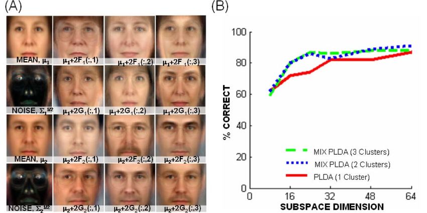
LI ET AL.: PROBABILISTIC MODELS FOR INFERENCE ABOUT IDENTITY                                                                                 149

Fig. 7. (a) Identification performance as with minimal preprocessing as a
function of signal and noise subspace size. (b) Identification perfor-
mance for progressive simplifications of the model.

then the conditional distribution is also Gaussian (see [6])
with mean and covariance

     P rðxp jxg Þ ¼ Gxp mp  1                  1
                              pp pg ðxg  mp Þ; pp : ð21Þ

It is possible to evaluate this Gaussian probability efficiently
(Appendix B, which can be found in the Computer Society
                                                                            Fig. 8. (a) Comparison of algorithms for the XM2VTS database. PLDA
Digital Library at http://doi.ieeecomputersociety.org/                      outperforms PCA [38], LDA [2], the Bayesian approach [28], Dual-Space
10.1109/TPAMI.2011.104), making the complexity of this                      (DS) LDA [39], and the probabilistic approach of Ioffe [19]
algorithm similar to that of the original LDA method.                       (b) Performance comparison for the XM2VTS lighting subset.
                                                                            (c) Comparison for the YALE database as a function of gallery images
    Example predictive distributions for the case where the                 (nearest neighbor approach) to RLDA [7], SLDA [7], LDA [2], and PCA
subspaces F and G are 1D are shown in Fig. 4B. The                          [38]. (d) Comparison for the ORL database.
learned face manifold (indicated in gray) is given by
P rðxÞ ¼ Gx ½; FFT þ GGT þ . A new gallery image in-                     dimension of the noise subspace has a more complex effect:
duces a Gaussian predictive distribution, with a mean that                  Performance is always worst when Dim(G) is zero and is
is projected onto the subspace spanned by the factor in F                   best when Dim(G) is roughly the same as Dim(F). Hence,
(dotted line). The projection direction depends on the noise                we set the signal and noise subspace size to be identical in
parameters  and the noise subspace G. To perform face                      all remaining experiments.
recognition, we would compare the likelihood of a new                           In Fig. 7b, we decompose the model into constituent
probe point under each of the predictive distributions. The                 parts. We force the noise  to be a multiple of the identity
likelihood for not matching either gallery image is found by                rather than diagonal (dashed versus solid lines). This
evaluating the probe point under the whole manifold                         reduces performance: The full algorithm learns which parts
distribution (gray area).                                                   of the image are most variable and downweights them in
                                                                            the decision. We also remove the noise subspace by setting
3.4 Experiment 1: Frontal Face Identification                               Dim(G) to zero (blue lines versus red lines), which
To explore the properties of the algorithm, we trained the                  decreases performance even further.
algorithm with all of the data from the first 195 individuals in                These restrictions can be easily related to other models.
the XM2VTS database. We tested with the last 100 indivi-                    When the covariance  is uniform and there is no noise
duals, using the one image from the first capture session as                subspace, the model takes the form of probabilistic PCA and
the gallery set and the one image from the last for the probe               the results are very similar to those for eigenfaces. In fact, the
set. Hence, the model must generalize from the training set                 PPCA model has very slightly superior performance due to
to new individuals.                                                         regularization induced by the prior over h. When we allow
   To ensure that the experiments are easy to replicate, we                 to have independent diagonal terms, the model takes the
used minimal preprocessing. Each image was segmented                        form of a factor analyzer. When we allow the noise subspace
with an iterative graph-cuts procedure. Three points were                   dimension Dim(G) to be nonzero and restrict  to be diagonal,
marked by hand. Faces were normalized to a standard                         our model is similar to that of Ioffe [19].
template using an affine transform. Final size was
70  70  3. Raw pixel values form the input vector. There                  3.4.1 Comparison to Other Algorithms
was no photometric normalization. For each probe, we                        In Fig. 8, we compare the performance of PLDA to other
compute the likelihood that it matches each face in the gallery             algorithms. We emphasize here that the preprocessing of
using (3). We calculate a posterior for the match, assuming                 the data is exactly the same in each case, so this is a pure test
uniform priors. We take the MAP solution as the match.                      of recognition ability when the remaining parts of the
   In Fig. 7a, we plot percent correct first match results as a             pipeline are held constant.
function of the subspace dimensions. For each line of the                      Fig. 8a shows that PLDA outperforms our implementa-
graph, the dimension of the signal Dim(F) is constant, but                  tions of five other algorithms on the XM2VTS database. The
the dimension of the noise Dim(G) varies. Increasing the                    closest competing methods are dual-space LDA [39] and the
signal dimension improves performance. Increasing the                       probabilistic approach of Ioffe [19].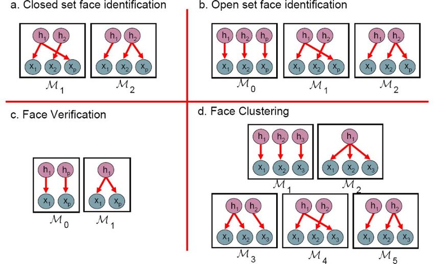
150 IEEE TRANSACTIONS ON PATTERN ANALYSIS AND MACHINE INTELLIGENCE, VOL. 34, NO. 1, JANUARY 2012
TABLE 1
Results for XM2VTS Database with N Gallery Images PCA,
LDA, Bayesian, and Unified Subspace Results from [25]
Bracketed results indicate results from our approach with automated
feature finding.
In Fig. 8b, we investigate performance for the same
algorithms on the lighting subset of the XM2VTS database.
The training set consisted of seven images each of the first
195 individuals and contained two lighting conditions. For
each individual, there were five images under frontal
lighting and two under side-lighting. The test set consisted
of 100 different individuals, where the gallery images were Fig. 9. Experiment 2: Clustering results for 80 frontal images consisting
taken from the first recording session and were under of four images each of 20 people. Blue lines divide clusters. The
frontal lighting and the probe images were taken from the algorithm has found 21 clusters—one of the original clusters has
erroneously been split.
fourth session and were lit from the side. All other
preprocessing was the same as for the original XM2VTS
consisting of image gradients at eight orientations and three
data. Once more, the PLDA algorithm outperforms the five
scales at points in a 6 6 grid around each keypoint. A
competing algorithms.
separate recognition model was built for each and these
In Fig. 8c, we present results from the Yale database,
were treated as independent.
which also contains lighting variation which was prepro-
Here, the training data consisted of images from the first
cessed as in [7]. We compare to published data from [7] and
three capture sessions from all 295 individuals in the
show that performance is superior to the RLDA, SLDA,
database. We use images from 1) capture session 1 or
LDA, and PCA algorithms. Finally, in Fig. 8d we compare
2) capture sessions 1-3 to form the gallery. We use images
results to the same algorithms on the ORL database (also as
from capture session 4 to form the probe set. This protocol
preprocessed by [7]), which contains both pose and lighting
was chosen to facilitate comparison with [25].
variation. Here the PLDA algorithm provides performance
With a single gallery image, peak performance was
that is comparable to SLDA and superior to RLDA, LDA,
99.7 percent: We misclassified one face (image 169.4.1)
and PCA. where the pose deviated from frontal. In Section 5, we
These experiments make a strong case for PLDA: Over present an algorithm to cope with pose changes. With three
four different databases and seven algorithms it produces gallery images we achieved 100 percent performance.
reliably better performance when all other parts of the face In Table 1, we compare PLDA performance to published
recognition pipeline are held constant. results from [25]. Here, the experimental protocol was
Our technique outperforms other LDA methods for three identical, but the whole preprocessing pipeline differs. Our
reasons. First, the per-pixel noise term means we have a method compares favorably to other algorithms, although
more sophisticated model of within-individual variation it is unwise to draw strong conclusions where the
(see Fig. 7b). Second, our method does not suffer from the difference in performance is only small. We believe that
small sample problem: The signal subspace F and noise Fig. 8 provides more information about the relative
subspace G may be completely parallel or entirely strengths of these algorithms. Nonetheless, these results
orthogonal. There is no need for two separate procedures suggest that PLDA can support strong recognition perfor-
as in the dual-space LDA algorithm [39]. Third, a slight mance and that the results of Fig. 8 were not just an artifact
benefit results from the regularizing effect of the prior over of the simple preprocessing.
the identity and noise variables.
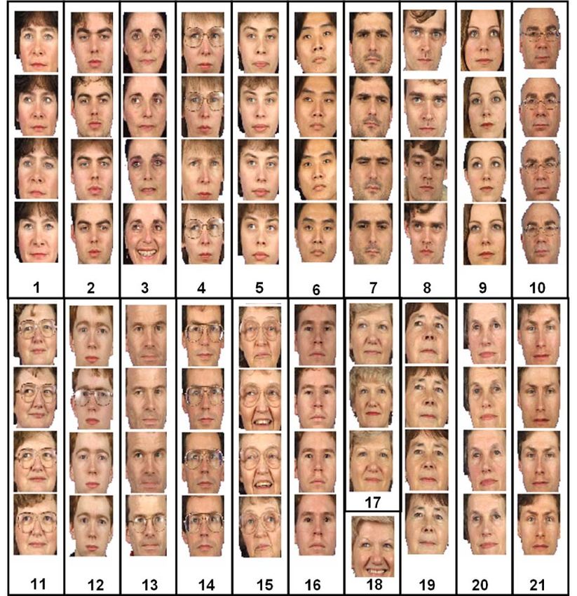
We also investigated identification performance for the 3.5 Experiment 2: Frontal Face Clustering
PLDA algorithm for the XM2VTS with more elaborate In Experiment 2 (Fig. 9), we demonstrate clustering using the
preprocessing. Eight keypoints on each face were identified elaborately preprocessed XM2VTS data. We train the system
by hand or automatically using the method described in using only the first 195 individuals from the XM2VTS
[34], depending on the condition. The images were database and signal and noise subspaces of size 64. The
registered using a piecewise triangular warp. The final algorithm is presented with 80 images taken from the last
image size was 400 400. We extracted feature vectors 100 individuals. In principle, it is possible to calculate the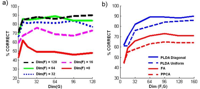
LI ET AL.: PROBABILISTIC MODELS FOR INFERENCE ABOUT IDENTITY                                                                              151

                                                                                                  TABLE 2
                                                                           Results of PLDA and Other State-of-the-Art Methods
                                                                                           for the LFW Database
                                                                       (Mean Classification Accuracy and Standard Error of the Mean)

                                                                       The top five rows are based on multiple descriptors and the bottom five
                                                                       rows are based on a single descriptor.
Fig. 10. Experiment 3 results: ROC curve of PLDA and other state-of-
the-art methods for face verification on LFW data set.
                                                                       protocol (e.g., [43] and [22]). In the “unrestricted configura-
                                                                       tion,” all available information, including the identities, can
likelihood for each possible clustering of the data using (19):        be used for training. The studies of [13], [37] used this
For example, we can calculate the likelihood that there are            configuration.
80 different individuals or that the 80 images are all of the             The aligned images were cropped to 80  150 pixels
same individual.                                                       following Nguyen and Bai [29]. Each image was normalized
   Unfortunately, in practice there are far too many possible          by passing it through a log function (logðx þ 1Þ) to suppress
configurations. Hence, we adopt a greedy agglomerative                 the effect of shadows and lighting. In addition, we localize
strategy. We start with the hypothesis that there are
                                                                       four keypoints following [10], [24] and estimate the facial
80 different individuals. We then consider merging all pairs
                                                                       pose by projecting the keypoint positions to the first
of individuals and choose the combination that increases
                                                                       principal component following [37]. The images of large
the likelihood the most. We continue this process until the
                                                                       right profile faces are swapped to left profile faces so that all
likelihood cannot be improved. In order to test the
                                                                       the images are left profile or near frontal. We investigated
clustering performance, we randomly select four images
                                                                       two types of descriptors on the aligned images: local binary
each from 20 individuals and apply our algorithm. We can
                                                                       patterns (LBP) [31] and three-patch local binary patterns
quantify performance by counting the number of splits and
                                                                       (TPLBP) [43]. We used the same parameters as [29], [37]. In
merges required to change our estimated clustering to the
                                                                       addition, we also investigated the SIFT descriptors com-
ground truth. Averaged over 100 data sets, the mean
                                                                       puted at the nine facial keypoints on the funneled images.
number of split/merges was 1.60.
                                                                       The SIFT data are available from [13]. The original
   Typical results are shown in Fig. 9 (here the number of
                                                                       dimensionality of the features was quite high (7,080 for
split/merges required is 1). The algorithm slightly over-
                                                                       LBP and TPLBP and 3,456 for SIFT), so we reduced the
partitions the data but does not erroneously associate
                                                                       dimension to 200 using PCA.
images from different individuals. We conclude that our
                                                                          For each pair of images, we compute the likelihood that
model can cope with complex compound decisions about
                                                                       they match each other using (3) and likelihood that they do
identity and can select model size without the need for
extra parameters.                                                      not match using (2). There are two views of the LFW
                                                                       database. The images in View 1 are used for model selection
3.6 Experiment 3: Face Verification                                    (subspace dimension of PLDA) and the images in View 2 are
In Experiment 3, we investigate face verification using the            used for training and test. We followed the “unrestricted
Labeled Faces in the Wild [18] database which contains                 configuration.” For each of the 10-fold cross-validation tests,
large variations in pose, expression, and lighting. Images             we used identities with at least two images for training. The
were grayscale and were prepared in two ways: 1) aligned               number of training images is around 8,000. A threshold of the
using commercial face alignment software by Taigman                    log-likelihood ratio is learned using 5,400 pairs of images in
et al. [37] and 2) funneled, which is available on the LFW             the nine folds of the data. The learned model is then tested
website [18]. There are a total of 13,233 images and 5,749             using the 600 pairs of held-out data. Table 2 and Fig. 10 are
people in the database. The number of images varies from               the comparison of PLDA with the state of the art methods on
one to 530 images.                                                     LFW database evaluated using average verification rate and
   The images are divided into 10 groups where the subject             ROC curves of the 10-fold cross-validation test, respectively,
identities are mutually exclusive. In each group, there are            where “u” and “r” denotes unrestricted and restricted
300 pairs of images from the same identity and 300 pairs               configuration, respectively.
from different identities. There are two possible training                The optimal subspace dimension of PLDA is 128, 96, and
configurations. In the “restricted configuration,” only the            48 for the LBP, TPLBP, and SIFT descriptors, respectively,
same/not-same labels are used no information about the                 and these settings were used in Table 2 and Fig. 10. The best
actual identities is used. Most previous work has restricted           performance of PLDA based on a single descriptor is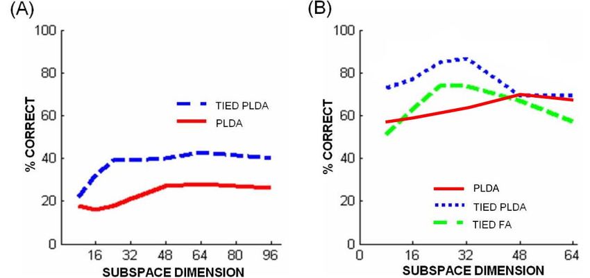
152                                  IEEE TRANSACTIONS ON PATTERN ANALYSIS AND MACHINE INTELLIGENCE,        VOL. 34,   NO. 1,   JANUARY 2012

87.3 percent using the LBP descriptor, which is 2.2 percent
better than the result of multishot learning (also using LBP)
in [37]. In addition, PLDA outperforms LDML using a
single SIFT descriptor [13] (3.0 percent higher in terms of
verification rate). Note that we have used the same SIFT
data as [13] and a similar LBP descriptor (but different
image size) as [37]. Therefore, the performance of our PLDA
model outperforms the current best model based on single
descriptor [37] that is reported on the result page of LFW
database [18].
   The combination of different descriptors is straightfor-
                                                                     Fig. 11. Mixtures of PLDA Model. (A) Graphical model relating data x to
ward for PLDA. We treat these descriptors independently              identities h, noise variables w, and parameters  ¼ f; F; G; g.
and the likelihoods of match and not-match are just the              (B) Predictive distribution for the subspace model with clusters. Each
product of those calculated on each descriptor. So it is             contains a 1D identity subspace (dotted lines) and one noise factor (not
                                                                     shown). The gray region represents face manifold. New gallery images
unnecessary to train another classifier such as SVM to do the        (red and green dots) induce predictive distributions that are themselves
final decision as in [43], [13], and [37]. The performance of        mixtures of Gaussians (red and green ellipses). The weight of ellipses
PLDA by combining LBP, TPLBP, and SIFT descriptors                   corresponds to weights of component.
(combined PLDA in Table 2 and Fig. 10) is 90.1 percent,
which was consistently better than that using each individual        two latent identity variables associated with an individual:
descriptor alone, agreeing with [43], [13], [37]. Furthermore,       The discrete variable ci determines which cluster the
this is better than the state of the art result: multishot [37]      individual belongs to and the identity vector hi determines
(89.5 percent) and LDML-MkNN [13] (87.5 percent) in the              the position within this cluster. For two faces to belong to the
unrestricted setting and High-Throughput Brain-Inspired              same individual, both of these variables must match.
(HTBI) Features [33] and CSML + SVM [29] in the restricted
                                                                     4.1 Learning and Recognition
setting. Note that the current top two methods in unrest-
ricted setting are based on four types of descriptors and it is      To learn the MixPLDA model we apply the standard recipe
                                                                     for learning mixtures of distributions (e.g., see [15] and [6]).
possible that PLDA’s performance might increase further if
                                                                     We embed the PLDA learning algorithm inside a second
we also introduced more discriminative descriptors.
                                                                     instance of the EM algorithm. In the E-Step, we find which
   We also note that multishot learning [37] needs to train
                                                                     cluster is responsible for each identity. In the M-Step, we learn
two classifiers during testing and the marginalized k
                                                                     the PLDA models for each cluster based on all of the
nearest neighbors (MkNN) [13] needs to find a set of
                                                                     associated data. More formally: 1) E-Step: For fixed
nearest neighbors. Compared to these methods, the PLDA
                                                                     F1...K ; G1...K ; 1...K , calculate the posterior probability P rðci ¼
algorithm is relatively efficient (see Appendix B, which can
                                                                     kjxij Þ that an individual i belongs to the kth cluster using the
be found in the Computer Society Digital Library at http://
                                                                     likelihood term in (19), where the matrix A has the same
doi.ieeecomputersociety.org/10.1109/TPAMI.2011.104).
                                                                     structure as in (13) and (14). 2) M-Step: For each cluster k, learn
   We encourage caution in comparing these results which
                                                                     the associated PLDA model using data weighted by the
compare pipeline to pipeline rather than algorithm to
                                                                     posterior probability of belonging to the cluster.
algorithm: The remaining differences may be due to                       Fig. 12A shows the results of learning a model from the
preprocessing or the recognition algorithm. We can con-              first 195 individuals in the XM2VTS database with minimal
clude that the PLDA algorithm can produce verification               preprocessing. For this case, we used K = 2 clusters and
results that are at least comparable to the state of the art         noise and identity subspaces of dimension 8. We used
using this challenging real-world database.                          10 iterations of the outer loop of the EM algorithm, and
                                                                     updated the PLDA model at each iteration with six
                                                                     iterations. Interestingly, the algorithm has organized the
4     MODEL 2: MIXTURES OF PLDAS
                                                                     clusters to separate men from women.
It is unrealistic to assume that the face manifold is well               In recognition, we again assess the probability that faces
modeled by a linear subspace. It is also unlikely that the noise     were generated from common underlying identity vari-
distribution is identical at each point in space. We resolve         ables. This now includes the choices of cluster ci as well as
these problems by describing the face manifold as a weighted         the position in that cluster hi . Once more, each of these
additive mixture of K PLDA distributions (see Fig. 11A):             quantities is fundamentally uncertain so we marginalize
                                                                   over all possible values. The analogue of (6) is
             P rðxij Þ ¼ Gx ci þ Fci hi þ Gci wij ; ci ;
             P rðhi Þ ¼ Gh ½0; I;                                     P rðxp ; xm Þ
                                                             ð22Þ            X K ZZZ
            P rðwij Þ ¼ Gw ½0; I;                                        ¼          P rðxp ; xm ; hm ; cm ; wp ; wm ; Þdhm dwp dwm :
          P rðci ¼ kÞ ¼ k    k ¼ f1 . . . Kg:                               cm ¼1

All terms have the same interpretation as before, but now                                                                               ð23Þ
there are k sets of parameters k ¼ fk ; Fk ; Gk ; k g. The term      Fig. 11B shows the data manifold (gray region) and
k is the prior probability of a measurement belonging to            predictive distributions (ellipses) for two data points. The
cluster k, where there are K clusters in total. There are now        predictive distributions are mixtures of Gaussians: There will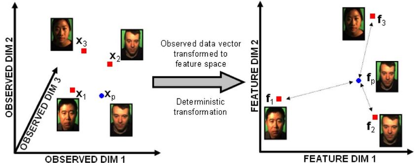
LI ET AL.: PROBABILISTIC MODELS FOR INFERENCE ABOUT IDENTITY                                                                                       153

                                                                            Fig. 13. Tied PLDA Model. (A) Graphical model relating data x to
Fig. 12. (A) Mixtures of the PLDA model. The top two rows show              identities h, noise variables w, and parameters  ¼ f; F; G; g.
elements of mixture component 1. The bottom two rows show                   (B) Predictive distribution for Tied model with two clusters. Each
component 2. Interestingly, the two clusters correspond to the two          contains a 1D identity subspace (dotted lines) and one noise factor (not
sexes. The mean of cluster 1 and images representing directions in the      shown). Gray region represents face manifold. A new gallery image (red
signal subspace all look like women (top row). For cluster 2 (row three),   dot) induces a predictive distribution that is a mixture of four Gaussians.
images all look like men. As before, different positions in the within-     Ellipse weight indicates weight of component in predictive distribution.
individual subspace (second and fourth row) look like different images of
the same person. (B) Identification results from MixPLDA model as a         In “tied” models [34], two or more viewing conditions are
function of subspace dimension.
                                                                            compared by assuming that they have a common under-
                                                                            lying variable hi , but different generation processes. For
be one contribution from each mixture component of the
model. However, many data points (e.g., green point) will be                example, consider viewing J images each of I individuals, at
almost entirely associated with the nearest mixture compo-                  K different poses. Here, we will assume that the pose k is
nent and will effectively have a Gaussian predictive distribu-              known for each observed datum xijk , although this is not
tion. Notice that this is quite a sophisticated model. The data             necessary. The generative model for this data is
manifold is nonlinear. The shape of the predictive distribu-
tion is complex and varies depending on the gallery data.                         P rðxijk jhi ; wijk Þ ¼ Gx ½k þ Fk hi þ Gk wijk ; k ;
                                                                                             P rðhi Þ ¼ Gh ½0; I;                               ð24Þ
4.2 Experiment 4
                                                                                           P rðwijk Þ ¼ Gw ½0; I:
In Experiment 4, we repeat the XM2VTS experiment (Fig. 8a)
for the mixture model. Percent correct performance improves                    The graphical model for Tied PLDA is given in
as we move from 1 to 2 clusters (Fig. 12B), but adding a third              Fig. 13A. Note that this model is quite different from the
does not make much difference. However, these results                       MixPLDA model. Both models describe the training data
should be treated with some caution: The two cluster                        as a mixture of factor analyzers. However, in the
mixPLDA model has twice as many parameters as the                           mixPLDA model, the representation of identity includes
original PLDA model. In principle, it is possible for the two               the choice of cluster ci . In the Tied PLDA model, the
clusters with N/2 dimensions to approximate the same                        representation of identity hi is constant (tied) regardless of
solution as the PLDA model with N dimensions. However,                      the cluster (viewing condition). Another way to think
the clusters found in Fig. 12A suggest that this did not                    about this is that the data are described as k clusters, but
happen.                                                                     certain positions in each cluster are “identity-equivalent.”
   The case would be clearer if we could investigate higher
dimensional subspaces and demonstrate a clear perfor-                       5.1 Learning and Recognition
mance benefit from the mixture model. Unfortunately, our                    Learning is very similar to the original PLDA model, with
ability to construct the between individual subspace F is                   one major difference. In the E-Step, we calculate the
limited by the number of individuals in the database (195).                 posterior distribution over the latent variables given
With three clusters of 64 dimensions, this only leaves
                                                                            the observed data as before. However, there is now a
1.01 people per dimension per cluster. Despite these
                                                                            separate M-Step for each cluster k in which the terms
concerns, we believe that the MixPLDA model is a
                                                                            k ; Fk ; Gk ; k are updated using only the data known to
promising method. It is fundamentally more expressive
than linear methods, and retains the advantages of the                      come from these clusters. A more detailed description of the
probabilistic approach.                                                     principles behind tied models can be found in [34].
   It would not have been easy to construct this model with                     We train using 195 individuals from the XM2VTS
a conventional distance-based approach. The representation                  database, with four frontal and four profile faces of each
of identity consists of one discrete variable ci and one                    individual. Fig. 14 shows the results of training the model
continuous variable hi and hence measurements of distance                   with two clusters using four frontal and four profile images
are no longer straightforward.                                              each from the first 195 individuals from the XM2VTS
                                                                            database with minimal preprocessing. The “tied” structure
                                                                            is reflected in the fact that the columns of F1 and F2 look
5    MODEL 3: TIED PLDA                                                     like images of the same people.
Although the above methods can cope with a considerable                         Recognition proceeds exactly as in the PLDA model, but
amount of image variation, there are some cases, such as                    now likelihood terms are calculated by marginalizing the
large pose changes, where viewing conditions are so                         joint likelihood implicitly defined by (24). The analogue of
disparate that a more powerful technique must be applied.                   (13) is
154 IEEE TRANSACTIONS ON PATTERN ANALYSIS AND MACHINE INTELLIGENCE, VOL. 34, NO. 1, JANUARY 2012
Fig. 15. Results for recognition across a 90 degree pose change using
Tied PLDA. (A) Experiment 5: Minimal preprocessing. (B) Experiment 6:
Full preprocessing. Results from PLDA and tied factor analysis model
[34] plotted for comparison.
Fig. 15B. Peak performance for our algorithm is 87 percent
which compares favorably to prior work by [34].
Fig. 14. Tied PLDA model for face recognition across pose. The
position hi in the identity subspace F is forced to be constant for both
In Table 3, we compare our method to other published
poses: As we move along the dimensions of the signal subspace, the results across different databases. Note that that most of the
basis functions look like the same person, regardless of pose (top two closest comparable algorithms (e.g., [4], [16], [34]) also use
rows). Position in the noise subspaces G is not tied, so these basis manual feature positioning.
functions are unrelated (bottom two rows).
2 3 5.3 Experiment 7: Cross-Pose Face Clustering
2 3 2 3 2 3 h 2 3
x1 k1 Fk1 Gk1 0 ... 0 6w1 7 1 In Experiment 7, we investigate clustering for the cross-pose
6x2 7 6 k2 7 6 Fk2 0 Gk2 ... 0 76 7 6 2 7 case using the elaborately preprocessed data. This is a
6 7 6 7 6 76w2 7 6 7
6 .. 7 ¼ 6 .. 7þ6 .. .. .. .. .. 76 7þ6 .. 7; challenging task involving compound recognition decisions
4.5 4 . 5 4 . . . . . 56 .. 7 4 . 5
4 . 5 across widely varying viewing conditions and a choice of
xN kn Fkn 0 0 . . . Gkn N
wN model order. Once more, we train with the first 195
ð25Þ individuals in the database. On each trial we select four
images each of 15 different individuals from the last 100
where Fkn indicates the factor matrix associated with the people in the database. Each image may be either frontal or
known pose of image n. profile and may come from any of the four recording
It is instructive to examine the predictive distribution for sessions. We cluster the data using the greedy agglomera-
a gallery image (Fig. 13B). If there are K viewing conditions tive method described in Section 3.5, replacing the PLDA
(clusters), then this will be a mixture of K 2 Gaussians. The model with the Tied PLDA model.
observed gallery datum may be associated with each of the Typical results are shown in Fig. 16. The algorithm
clusters (it may be in any pose). For each possible successfully identified most clusters regardless of whether
association, it makes a prediction in every cluster (the the faces are all frontal, all profile, or a mix of both (10/15
probe image may also be in any pose). When the pose of the clusters are correct). The number of splits and merges
probe and gallery are known, the predictive distribution required to move to the correct clustering for this example
becomes just a single Gaussian. is 8, which is slightly worse than the experimental average
5.2 Experiments 5-6: Cross-Pose Identification of 7.32 over 100 repetitions.
In Experiment 5, we use full images with the same minimal
preprocessing as in Experiment 1. We trained using the first 6 MANUAL VERSUS AUTOMATIC KEYPOINTS
195 individuals from the XM2VTS database and test using a Throughout this paper, we constructed models using
single frontal gallery image and right-profile probe image manually localized image keypoints. We take this approach
from the remaining 100 individuals in the database. These as it makes the results easier to replicate and defines a clear
are taken from the first and fourth recording session, upper bound on performance. However, it might be that
respectively. The pose is assumed to be known. In Fig. 15A,
we plot percent correct first match results as a function of
the subspace dimension for both the tied PLDA and PLDA TABLE 3
models. The tied PLDA model doubles performance but Results for Percent Correct Face Identification
only from roughly 20 to 40 percent. across Large Pose Changes
In Experiment 6, we apply the elaborate preprocessing
method from Experiment 1. However, as in the previous
experiment, we train using the first 195 individuals and test
with the last 100. Three of the original eight keypoint
positions are occluded in the profile model. We omit these
and add one more feature on the right side of the face to Number of gallery images given in brackets after database name.
compensate. Identification performance is plotted in Bracketed results from our approach with automated feature finding.LI ET AL.: PROBABILISTIC MODELS FOR INFERENCE ABOUT IDENTITY 155
Fig. 17. Experiments 4 and 7 are repeated with automatically localized
features (using the method of [34]). Performance declines slightly but
remains very high.
sources such as image submodels or data from different
biometric domains without the need to learn weights.
There have been other probabilistic algorithms for face
recognition, most notably the work of Liu and Wechsler
[26] and Moghaddam et al. [28], which we considered in
Section 1.2. Zhou and Chellapa [46] presented a system
which also acknowledged uncertainty in the identity
representation, but inference was quite different and did
Fig. 16. Experiment 7: Clustering results for 60 frontal and profile not produce a posterior probability over matches.
images, consisting of four images each of 15 people. Blue lines divide The most closely related work to this paper is by Ioffe
clusters, red boxes indicate images erroneously associated with the [19] who presented a similar algorithm to Model 1, which
wrong group. The algorithm found 20 clusters. Several clusters have
erroneously been split (bottom right) and two erroneously merged (red
he also termed probabilistic linear discriminant analysis.
boxes). In this case, we would require eight splits and merges to The main differences are: 1) His model requires projection
associate the data correctly. of the data down onto a few principal components rather
than modeling the original data vector and is hence not a
our models are unusually susceptible to inaccurate keypoint fully probabilistic description of the data. If the dimensions
localization. In order to check that this was not the case, we of the data have very different scales, it is quite possible to
repeated the frontal and cross-pose XM2VTS experiments erroneously throw out critical information with this
using gallery images that were manually labeled, but probe approach. 2) There is no equivalent of the per-pixel noise
images that were automatically labeled using the method of vector (and hence it misses out on the performance gain
[34]. The results can be seen in Fig. 17. Performance declines illustrated in Fig. 7b): The results of Ioffe’s algorithm are
slightly with automatic labeling, but is still very high. Our consequently very similar to the blue dashed line in this
feature localizer is not particularly sophisticated and it is figure. 3) He proposes a closed form learning algorithm. No
such solution is known for the PLDA models proposed here
likely that these results could be improved upon.
with diagonal covariance—to get the extra performance
boost of our method we must resort to iterative optimiza-
7 DISCUSSION tion techniques such as the EM algorithm.
In this paper, we have presented a series of probabilistic The tied PLDA model is a generalization of Tied Factor
models for face recognition. Our key contribution is a Analysis [34]. The latter model uses a bilinear mechanism to
probabilistic approach to LDA that sidesteps the small- compare images across disparate viewing conditions. Tied
sample problem and has a more sophisticated noise model. PLDA uses the same mechanism, but additionally models a
We have demonstrated that there are empirical reasons to within-individual subspace in each viewing condition. This
favor our approach for both frontal and cross-pose face is shown to improve matching performance across large
recognition. Linear discriminant analysis is a very general pose differences.
technique and this method could find application in many
other areas of computer vision. Our probabilistic approach 7.2 Further Work
also leads to two nonlinear extensions that are more Many other methods can also be understood in terms of LIVs.
expressive: mixtures of PLDA models and tied PLDA models. For example, distance-based methods based on independent
components analysis [1] have a clear generative interpreta-
7.1 Relation to Other Methods tion. The models described here have been purely statistical
A probabilistic framework is beneficial for several reasons. in nature. However, a sensible future research direction
First, the posterior distribution provides a measure of the would be to combine this form of inference with work which
uncertainty on the decision. Second, we can apply priors to attempts to formally model the physical process of face
different matching hypotheses. For example, in a surveillance image creation, such as that of Blanz et al. [5].
system, identification in one camera could be used to modify Some successful approaches to face recognition in un-
the prior probability of the same person appearing in a nearby constrained conditions (e.g., [11], [30]) do not build a
camera. Third, probabilities make it easy to combine different probabilistic description of the data, but seek discriminativeYou can also read