Demand Forecasting for Platelet Usage: from Univariate Time Series to Multivariate Models
←
→
Page content transcription
If your browser does not render page correctly, please read the page content below
Demand Forecasting for Platelet Usage: from Univariate Time
Series to Multivariate Models
arXiv:2101.02305v1 [cs.LG] 6 Jan 2021
Maryam Motamedia,∗ , Na Lia,b , Douglas G. Downa and Nancy M. Heddleb,c
a Department of Computing and Software, McMaster University, Hamilton, Ontario L8S 4L8, Canada
b McMaster Centre for Transfusion Research, Department of Medicine, McMaster University, Hamilton, Ontario L8S 4L8,
Canada
c Centre for Innovation, Canadian Blood Services, Ottawa, Ontario K1G 4J5, Canada
E-mail: motamedm@mcmaster.ca [Motamedi]; lin18@mcmaster.ca [Li];
downd@mcmaster.ca [Down]; heddlen@mcmaster.ca [Heddle]
Abstract
Platelet products are both expensive and have very short shelf lives. As usage rates for platelets are highly variable,
the effective management of platelet demand and supply is very important yet challenging. The primary goal of
this paper is to present an efficient forecasting model for platelet demand at Canadian Blood Services (CBS). To
accomplish this goal, four different demand forecasting methods, ARIMA (Auto Regressive Moving Average),
Prophet, lasso regression (least absolute shrinkage and selection operator) and LSTM (Long Short-Term Memory)
networks are utilized and evaluated. We use a large clinical dataset for a centralized blood distribution centre for
four hospitals in Hamilton, Ontario, spanning from 2010 to 2018 and consisting of daily platelet transfusions along
with information such as the product specifications, the recipients’ characteristics, and the recipients’ laboratory
test results. This study is the first to utilize different methods from statistical time series models to data-driven
regression and a machine learning technique for platelet transfusion using clinical predictors and with different
amounts of data. We find that the multivariate approaches have the highest accuracy in general, however, if suffi-
cient data are available, a simpler time series approach such as ARIMA appears to be sufficient. We also comment
on the approach to choose clinical indicators (inputs) for the multivariate models.
Keywords: demand forecasting; time series forecasting; platelet products; blood demand and supply chain; long short-term
memory networks
∗ Author to whom all correspondence should be addressed (e-mail: motamedm@mcmaster.ca).
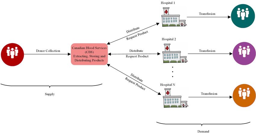
11. Introduction Platelet products are a vital component of patient treatment for bleeding problems, cancer, AIDS, hep- atitis, kidney or liver diseases, traumatology and in surgeries such as cardiovascular surgery and organ transplants (Kumar et al., 2015). In addition, miscellaneous platelet usage and supply are associated with several factors such as patients with severe bleeding, trauma patients, aging population and emergence of a pandemic like COVID-19 (Stanworth et al., 2020). The first two factors affect the uncertain demand pattern, while the latter two factors result in donor reduction. Platelet products have five to seven days shelf life before considering test and screening processes that typically last two days (Fontaine et al., 2009). The extremely short shelf life along with the highly variable daily platelet usage makes platelet demand and supply management a highly challenging task, invoking a robust blood product demand and supply system. To deal with high demand variation, hospitals usually hold excess inventory. However, holding surplus inventory makes platelet demand forecasting even more challenging for blood distribution centres. In particular, holding excessive platelet inventory in hospital blood banks not only results in a high wastage rate, but also prevents the blood suppliers from realizing the real underlying platelet demand. which in turn yields an inefficient demand forecasting system. This can result in the bullwhip effect, the increased variation in demand as a result of moving upstream in the supply chain (Croson and Donohue, 2006). This effect arises in a number of domains, including grocery supply chains (Dejonckheere et al., 2004) as well as in healthcare service-oriented supply chains (Samuel et al., 2010; Rutherford et al., 2016). The bullwhip effect is inevitable in a healthcare system, since for the blood products, specifically platelet products with extremely short shelf lives, hospitals tend to order more than their regular demand to ensure that they can meet the actual demand, as shortages must be avoided (they can put patients at risk). Apart from this bullwhip effect, there are many uncertainties faced by blood centres due to the high demand variation. Since platelet products are perishable, high inventory levels result in excessive wastage, something that could be mitigated with better demand forecasting. On the other hand, low inventory levels increase the risk of shortages resulting in urgent delivery costs. Accordingly, accurately forecasting the demand for blood products is a core requirement of a robust blood demand and supply management system. Two organizations, CBS and Héma-Québec, are responsible for providing blood products and ser- vices in transfusion and transplantation for Canadian patients. The former operates within all Canadian provinces and territories excluding Québec, while the latter is in charge of the province of Québec. The current blood supply chain for CBS is an integrated network consisting of a regional CBS distribution centre and several hospitals, as illustrated in Fig. 1. Currently, there are nine regional blood centres oper- ating for CBS, each covering the demand for several hospitals (Hospital Liaison Specialists, [Accessed Date: 2020-11-01). Hospitals request blood products from the regional blood centres for the next day, yet, the regional blood centres are not aware of the actual demands as each hospital has its own blood bank. Furthermore, recipients’ demographic and hospitals’ inventory management systems are not dis- closed to CBS or the regional blood centres. This results in a high wastage rate for the hospitals (about 6% in Hamilton, Ontario) and CBS (about 15% and has seasonal variation), which may be partly due to the bullwhip effect. This research is motivated by the platelet management problem confronted by CBS. There are several issues faced by CBS, making the platelet management problem difficult. As mentioned above, CBS cur-
Fig. 1: CBS blood supply chain with one regional blood centre and multiple hospitals

rently does not have access to transfused patients’ demographics. Also, owing to the lack of information
transmission between CBS and hospitals, the effect of clinical changes on platelet demand cannot be
tracked by CBS. The need for robust and accurate platelet demand forecasting calls for transparency of
information between CBS and hospitals. In this research, we forecast platelet demand to overcome these
challenges.
   We study a large clinical database with 61377 platelet transfusions for 47496 patients in hospitals
in Hamilton, Ontario from 2010 to 2018. We analyse the database to extract trends and patterns, and
find relations between the demand and clinical indicators. We find that there are three key issues that
should be considered in the demand forecasting process: seasonality, the effect of clinical indicators
on demand, and nonlinear correlations among these clinical indicators. Consequently, we progressively
build four demand forecasting models (of increasing complexity) that address these issues. The proposed
methods are applied on the data to determine the influence of demand history as well as clinical indicators
on demand forecasting. The first two methods are univariate time series that only consider the demand
history, while the remaining two methods, multivariate regression and machine learning, consider clinical
indicators. These four methods are utilized to pursue the following goals: i) more precise platelet demand
forecasting resulting in increased information transparency between CBS and hospitals, ii) reducing the
bullwhip effect, as a consequence of effective demand forecasting; iii) investigating the impact of clinical
indicators on the platelet demand; and iv) having a robust forecasting model for platelet demand which
accounts for variation in multiple factors. The main contributions of this study are as follows:
1. We analyze the time series of platelet transfusion data by decomposing it into trend, seasonality and
   residuals, and detect meaningful patterns such as weekday/weekend and holiday effects that should
   be considered in any platelet demand predictor.
2. We utilize four different demand forecasting methods from univariate time series methods to multi-
   variate methods including regression and machine learning. Since CBS has no access to recipients’
   demographic data, our first method, ARIMA, only considers demand history for forecasting, while the
second model, Prophet, includes seasonalities, trend changes and holiday effects. We found that these
   models have issues with respect to accuracy, in particular when a limited amount of data are available,
   accordingly we apply a lasso regression method to include clinical indicators for demand forecast-
   ing. Finally, LSTM networks are used for demand forecasting to explore the nonlinear dependencies
   among the clinical indicators and the demand.
3. We utilize clinical indicators in the demand forecasting process, and select those that are most impact-
   ful through a structural variable selection and regularization method called lasso regression. Results
   show that incorporating the clinical indicators in demand forecasting enhances the forecasting accu-
   racy.
4. We investigate the effect of different amounts of data on the forecasting accuracy and model perfor-
   mance and provide a holistic evaluation and comparison for different forecasting methods to evalu-
   ate the effectiveness of these models for different data types, providing suggestions on using these
   robust demand forecasting strategies in different circumstances. Results show that by having a lim-
   ited amount of data (two years in our case), multivariate models outperform the univariate models,
   whereas having a large amount of data (eight years in our case) results in the ARIMA model perform-
   ing nearly as well as the multivariate methods.
  The rest of this paper is organized as follows. Section 2 provides an initial exploration of the data. In
Section 3 we provide a literature review of demand forecasting methods for blood products, with a focus
on platelets. We provide the data description, model background, model development and evaluation of
four different models for platelet demand forecasting in Section 4. In Section 5, a comparison of the
models is provided, and finally, in Section 6, concluding remarks are provided, including a discussion of
ongoing work for this problem.

2. Problem Definition

In this study, we consider a blood supply system consisting of CBS and four major hospitals operating
in Hamilton, namely, Hamilton General Hospital, Juravinski Hospital, McMaster University Medical
Centre (MUMC), and St. Joseph’s (STJ) Healthcare Hamilton. These hospital blood banks operate with
a Transfusion Medicine (TM) laboratory team to manage blood product transfusions to patients. Platelet
products are collected and produced at CBS and after testing for viruses and bacteria (a process which
lasts two days), platelets are ready to be shipped to hospitals and transfused to patients. At the beginning
of the day, hospitals receive platelet products that were ordered on the previous day, from CBS. In the
case of shortages, hospitals can place expedited (same-day) orders at a higher cost. Prior to September
2017, platelets had five days of shelf life, while after this date, the shelf life of platelets was increased
to seven days. After passing the shelf life, platelet products are expired and discarded. Given the high
shortage and wastage costs, forecasting short-term demand for platelets is of particular value.
   In order to propose a short-term demand forecasting model for CBS, we first explore the data for
identifying temporal (daily/monthly) patterns that can inform our demand forecasting techniques. This
initial analysis ranges from 2010/01/01 to 2018/12/31. An initial observation is that the demand is highly
variable, with a transfused daily average of 17.90 units and a standard deviation of 7.05 units.
   In terms of specific temporal patterns, we first looked into the daily platelet usage patterns by year,
month and day. There are no specific yearly patterns for platelet transfusions. Fig. 2(a) illustrates the
                         50


                         40
Daily Units Transfused

                                                                                                                                     'DLO\8QLWV7UDQVIXVHG
                         30


                         20

                         10

                         0

                              January   February   March    April   May   June   July   August September October November December
                                                                           Month                                                                                                           0RQGD\   7XHVGD\   :HGQHVGD\   7KXUVGD\         )ULGD\   6DWXUGD\   6XQGD\
                                                                                                                                                                                                                                        'D\RIWKHZHHN
                                                                      (a) Month                                                                                                                                                       (b) Weekday

                                                           Fig. 2: Boxplots for mean daily units transfused in week, month and year

daily platelet usage pattern by month. It indicates that the platelet usage varies by month, the lowest
number of transfusions is in January while the highest number of transfusions is in July (January = mean
[sd(standard deviation)]: 17.35 [6.43], July = mean [sd]: 20.38 [8.03]). It is worth noticing that in July,
the number of outliers (points outside of the whiskers in the boxplot) is also higher in comparison to
other months. Outliers are defined as points with values greater than the third quartile plus 1.5 times the
interquartile range or less than the first quartile minus 1.5 times the interquartile range. As we can see
from Fig. 2(a), there is significant monthly seasonality (one-way ANOVA, F = 3.94, P value
demand predictor.
7UDQVIXVHG
5HFHLYHG
'DLO\8QLWV
in this period, and it becomes stationary from 2016 onwards. As a result, we will train our models in two
scenarios, one with the whole dataset and the other by using the data ranging from 2016 to 2018.
                       10 15 20 25 30 35
            data

                                                                                                              4
                                                                                                              2
            seasonal

                                                                                                              0
                                                                                                              −2
                                                                                                              −4
                       19
            trend
                       18
                       17
                       16

                                                                                                              15
                                                                                                              10
            residual

                                                                                                              5
                                                                                                              0
                                                                                                              −5
                                           2010          2012           2014          2016             2018
                                                                               time

                                                  Fig. 4: Time series decomposition using STL method

3. Literature Review

There is a limited literature on platelet demand forecasting; most investigates univariate time series meth-
ods. In these studies, forecasts are based solely on previous demand values, without considering other
features that may affect the demand. Frankfurter et al. (1974) develop transfusion forecasting models
using Exponential Smoothing (ES) methods for a blood collection and distribution centre in New York.
Critchfield et al. (1985) develop models for forecasting platelet usage in a blood centre using several
time series methods including Moving Average (MA), Winter’s method and ES. Silva Filho et al. (2012)
develop a Box-Jenkins Seasonal Autoregressive Integrated Moving Average (BJ-SARIMA) model to
forecast weekly demand for blood components in hospitals. Their proposed method, SARIMA, is based
on a Box-Jenkins approach that takes into consideration the seasonal and nonseasonal characteristics of
time series data. Later, Silva Filho et al. (2013) extend their model by developing an automatic procedure
for demand forecasting while also changing the level of the model from hospital level to regional blood
centre in order to help managers use the model directly. Kumari and Wijayanayake (2016) propose a
blood inventory management model for the daily supply of platelets focusing on reducing platelet short-
ages. Three time series methods, namely MA, Weighted Moving Average (WMA) and ES are used to
forecast the demand, and are evaluated based on shortages. Fortsch and Khapalova (2016) test various
approaches to predict blood demand such as Naı̈ve, moving average, exponential smoothing, and mul-
tiplicative Time Series Decomposition (TSD), among them a Box-Jenkins (ARMA) approach, which
uses an autoregressive moving average model, results in the highest prediction accuracy. They forecast
total blood demand as well as individual blood type demands, a feature that differentiates their method.
Lestari et al. (2017) apply four models to forecast blood components demand including moving average,
weighted moving average, exponential smoothing, exponential smoothing with trend, and select the best
method for their data based on the minimum error between forecasts and the actual values. Volken et al. (2018) use generalized additive regression and time-series models with exponential smoothing to predict future whole blood donation and RBC transfusion trends. Several recent studies take clinically-related indicators into consideration. Drackley et al. (2012) esti- mate long-term blood demand for Ontario, Canada based on previous transfusions’ age and sex-specific patterns. They forecast blood supply and demand for Ontario by considering demand and supply pat- terns, and demographic forecasts, with the assumption of fixed patterns and rates over time. Khaldi et al. (2017) apply Artificial Neural Networks (ANNs) to forecast the monthly demand for three blood com- ponents, red blood cells (RBCs), platelets and plasma for a case study in Morocco. Guan et al. (2017) propose an optimization ordering strategy in which they forecast the platelet demand for several days into the future and build an optimal ordering policy based on the predicted demand, concentrating on minimizing the wastage. Their main focus is on an optimal ordering policy and they integrate their de- mand model in the inventory management problem, meaning that they do not try to precisely forecast the platelet demand. Li et al. (2020) develop a hybrid model consisting of seasonal and trend decomposition using Loess (STL) time series and eXtreme Gradient Boosting (XGBoost) for RBC demand forecasting and incorporate it in an inventory management problem. In this study, we utilize multiple demand forecasting methods, including univariate analysis (time series methods) and multivariate analysis (regression and machine learning methods), and evaluate the performance of these models for platelet demand forecasting. Moreover, in contrast with earlier studies, we explore the value gained from including a range of clinical indicators for platelet demand forecasting. More specifically, we consider clinical indicators, consisting of laboratory test results, patient character- istics and hospital census data as well as statistical indicators, including the previous week’s platelet usage and previous day’s received units. In addition to the linear effects of the clinical indicators, we study the nonlinear effect of these clinical indictors in our choice of machine learning model. Results indicate that platelet demand is dependent on the clinical indicators and therefore including them in the demand forecasting process enhances the accuracy. Moreover, we explore the effect of having different amounts of data on the accuracy of the forecasting methods. To the best of our knowledge, this study is the first that utilizes and evaluates different demand forecasting methodologies from univariate time series to multivariate models for platelet products and explores the effect of the amount of available data on these approaches. 4. Demand Forecasting 4.1. Data Description The data in this study are constructed by processing CBS shipping data and the TRUST (Transfusion Research for Utilization, Surveillance and Tracking) database at the McMaster Centre for Transfusion Research (MCTR) for platelet transfusion in Hamilton hospitals. The study is approved by the Canadian Blood Services Research Ethics Board and the Hamilton Integrated Research Ethics Board. The dataset ranges from 2010 to 2018 and consists of 61377 transfusions for 47496 patients in Hamil- ton, 48190 transfusions to inpatients and 13187 to outpatients. It is high dimensional, with more than 100 variables that can be divided into four main groups: 1. the transfused product specifications such as
product name and type, received date, expiry date, 2. patient characteristics such as age, gender, patient
ABO Rh blood type, 3. the transfusion location such as intensive care, cardiovascular surgery, hema-
tology, and 4. available laboratory test results for each patient such as platelet count, hemoglobin level,
creatinine level, and red cell distribution width.
   The data for analysis are processed in two steps: in the first step, we have the granular data that
includes all of the platelet transfusions. Each row contains product-related information, the recipient’s
characteristics, hospital location information and lab tests. In the second step, a daily-aggregated dataset
is constructed with each row containing the daily product, patient-related and location information along
with the aggregated lab tests. In the daily aggregated dataset, 170 processed variables are included using
straightforward statistical transformations (e.g. mean, min, max, sum).
   Additionally, we add new variables such as the number of platelet transfusions in the previous day and
previous week, the number of received units in the previous day, and day of the week. Table 1 gives the
set of variables that are used in this study along with their descriptions. These variables are selected by a
lasso regression model (Tibshirani, 1996) which is explained in detail in Section 4.4. Since the ABO Rh
blood type compatibility between the patient and the product is not necessary (although preferable) for
platelet transfusion, it is not considered as a model variable.
   One of the data characteristics is that data variables, in particular abnormal laboratory test results, are
highly correlated, as shown in Fig. 5. These high correlations give rise to some challenges when data
variables are considered in the demand forecasting process, as will be seen in Section 4.4.
   As we can see from Table 1, data variables have different ranges, and hence are standardized by
removing the mean and scaling to unit variance by yi = (xi − ui )/si , where x is the variable, u is its mean
and s is its standard deviation. All data processing and analysis and model implementations are carried
out using the Python 3.7 programming language. We implement four models and train them for two
scenarios. In the first scenario, we train each model for two years of data from 2016 to 2017 and we use
data from 2018 for testing. In the second scenario, each model is trained with data from 2010 to 2017
for eight years, and is tested with 2018 data. We use Mean Absolute Percentage Error (MAPE) and Root
Mean Square Error (RMSE) to evaluate model performance.

4.2. The ARIMA model

An autoregressive integrated moving average model consists of three components, an autoregressive
(AR) component that considers a linear combination of lagged values as the predictors, a moving average
(MA) component of past forecast errors (white noise), and an integrated component where differencing
is applied on the data to make it stationary. Let y1 , y2 , . . . , yt be the observations over time period t; the
time series can be written as:

      yt = f (yt−1 , yt−2 , yt−3 , . . . , yt−n ) + εt                                                        (1)

An ARIMA model assumes that the value of an observation is a linear function of a number of previous
past observations and stochastic terms. The stochastic term, εt , is independent of previous observations
and is identically distributed for each t, following a normal distribution with zero mean. The ARIMA
Table 1: Data variable definition and description
Name Description
abnormal ALP Number of patients with abnormal alkaline phosphatase
abnormal MPV Number of patients with abnormal mean platelet volume
abnormal hematocrit Number of patients with abnormal hematocrit
abnormal PO2 Number of patients with abnormal partial pressure of oxygen
abnormal creatinine Number of patients with abnormal creatinine
abnormal INR Number of patients with abnormal international normalized ratio
abnormal MCHb Number of patients with abnormal mean corpuscular hemoglobin
abnormal MCHb conc Number of patients with abnormal mean corpuscular hemoglobin concentration
abnormal hb Number of patients with abnormal hemoglobin
abnormal mcv Number of patients with abnormal mean corpuscular volume
abnormal plt Number of patients with abnormal platelet count
abnormal redcellwidth Number of patients with abnormal red cell distribution width
abnormal wbc Number of patients with abnormal white cell count
abnormal ALC Number of patients with abnormal absolute lymphocyte count
location GeneralMedicine Number of patients in general medicine
location Hematology Number of patients in hematology
location IntensiveCare Number of patients in intensive care
location CardiovascularSurgery Number of patients in cardiovascular surgery
location Pediatric Number of patients in pediatrics
Monday Indicating the day of the week
Tuesday Indicating the day of the week
Wednesday Indicating the day of the week
Thursday Indicating the day of the week
Friday Indicating the day of the week
Saturday Indicating the day of the week
Sunday Indicating the day of the week
lastWeek Usage Number of units transfused in the previous week
yesterday Usage Number of platelet units transfused in the previous day
yesterday ReceivedUnits Number of units received by the hospital in the previous day
model can be written as:
yt = µ + ϑ1 yt−1 + ϑ2 yt−2 + ϑ3 yt−3 + · · · + ϑ p yt−p + εt
− φ1 εt−1 − φ2 εt−2 − φ3 εt−3 − · · · − φq εt−q (2)
where µ is a constant, ϑi and φ j are model parameters in which i = 1, 2, . . . , p and j = 0, 1, 2, . . . , q, p
and q are the model orders and define the number of autoregressive terms and moving average terms,1.0
abnormal_ALP 1 0.34 0.46 0.25 0.34 0.41 0.26 0.18 0.4 0.35 0.45 0.39 0.34 0.33 0.27 0.25 0.33 0.13 0.18 0.1 0.083 0.078 0.12 0.1 -0.048-0.089 0.22 0.17 0.12
abnormal_mpv 0.34 1 0.68 0.53 0.41 0.66 0.44 0.43 0.62 0.52 0.64 0.45 0.46 0.38 0.45 0.35 0.36 0.37 0.25 0.12 0.18 0.16 0.15 0.18 -0.14 -0.14 0.24 0.21 0.14
abnormal_hematocrit 0.46 0.68 1 0.61 0.53 0.8 0.39 0.26 0.84 0.64 0.81 0.62 0.53 0.46 0.53 0.46 0.45 0.41 0.26 0.14 0.22 0.18 0.19 0.21 -0.16 -0.16 0.28 0.26 0.19
abnormal_pO2 0.25 0.53 0.61 1 0.41 0.61 0.28 0.15 0.57 0.39 0.5 0.34 0.51 0.25 0.34 0.071 0.34 0.7 0.12 0.12 0.21 0.2 0.17 0.13 -0.18 -0.22 0.04 0.15 0.11
0.8
abnormal_creatinine 0.34 0.41 0.53 0.41 1 0.53 0.25 0.19 0.57 0.34 0.56 0.39 0.46 0.33 0.31 0.22 0.49 0.28 0.095 0.062 0.16 0.16 0.12 0.13 -0.065-0.085 0.17 0.24 0.17
abnormal_INR 0.41 0.66 0.8 0.61 0.53 1 0.42 0.28 0.83 0.6 0.91 0.55 0.51 0.41 0.62 0.56 0.37 0.55 0.35 0.18 0.25 0.26 0.24 0.25 -0.26 -0.26 0.26 0.27 0.18
abnormal_MCHb 0.26 0.44 0.39 0.28 0.25 0.42 1 0.54 0.4 0.61 0.4 0.36 0.33 0.28 0.26 0.28 0.23 0.22 0.17 0.087 0.11 0.091 0.099 0.13 -0.1 -0.1 0.2 0.16 0.11
abnormal_MCHb_conc 0.18 0.43 0.26 0.15 0.19 0.28 0.54 1 0.3 0.26 0.29 0.26 0.23 0.22 0.18 0.21 0.21 0.095 0.1 0.063 0.08 0.1 0.037 0.049-0.051-0.052 0.19 0.11 0.067
0.6
abnormal_hb 0.4 0.62 0.84 0.57 0.57 0.83 0.4 0.3 1 0.55 0.84 0.53 0.48 0.41 0.47 0.53 0.46 0.46 0.27 0.15 0.21 0.22 0.2 0.21 -0.16 -0.19 0.25 0.26 0.19
abnormal_mcv 0.35 0.52 0.64 0.39 0.34 0.6 0.61 0.26 0.55 1 0.59 0.42 0.33 0.36 0.41 0.4 0.27 0.26 0.27 0.11 0.17 0.11 0.15 0.17 -0.14 -0.13 0.27 0.23 0.14
abnormal_plt 0.45 0.64 0.81 0.5 0.56 0.91 0.4 0.29 0.84 0.59 1 0.59 0.47 0.45 0.61 0.6 0.43 0.39 0.35 0.17 0.23 0.24 0.21 0.23 -0.21 -0.21 0.31 0.29 0.19
abnormal_redcellwidth 0.39 0.45 0.62 0.34 0.39 0.55 0.36 0.26 0.53 0.42 0.59 1 0.42 0.35 0.47 0.31 0.29 0.23 0.26 0.1 0.12 0.15 0.13 0.19 -0.16 -0.12 0.16 0.18 0.13
0.4
abnormal_wbc 0.34 0.46 0.53 0.51 0.46 0.51 0.33 0.23 0.48 0.33 0.47 0.42 1 0.22 0.37 0.14 0.36 0.35 0.19 0.08 0.15 0.13 0.12 0.13 -0.091 -0.11 0.12 0.15 0.12
abnormal_ALC 0.33 0.38 0.46 0.25 0.33 0.41 0.28 0.22 0.41 0.36 0.45 0.35 0.22 1 0.19 0.29 0.36 0.11 0.12 0.093 0.062 0.082 0.071 0.098-0.013-0.021 0.24 0.17 0.11
location_GeneralMedicine 0.27 0.45 0.53 0.34 0.31 0.62 0.26 0.18 0.47 0.41 0.61 0.47 0.37 0.19 1 0.1 0.053 0.28 0.35 0.16 0.22 0.18 0.095 0.26 -0.3 -0.28 0.09 0.1 0.039
location_Hematology 0.25 0.35 0.46 0.071 0.22 0.56 0.28 0.21 0.53 0.4 0.6 0.31 0.14 0.29 0.1 1 0.042 0.099 0.21 0.097 0.06 0.096 0.16 0.14 -0.066-0.035 0.3 0.21 0.15
0.2
location_IntensiveCare 0.33 0.36 0.45 0.34 0.49 0.37 0.23 0.21 0.46 0.27 0.43 0.29 0.36 0.36 0.053 0.042 1 -0.012 0.11 0.075 0.063 0.078 0.09 0.073 0.022 0.025 0.21 0.2 0.14
location_CardiovascularSurgery 0.13 0.37 0.41 0.7 0.28 0.55 0.22 0.095 0.46 0.26 0.39 0.23 0.35 0.11 0.28 0.099-0.012 1 0.073 0.11 0.24 0.21 0.14 0.1 -0.23 -0.280.000270.097 0.075
location_Pediatric 0.18 0.25 0.26 0.12 0.095 0.35 0.17 0.1 0.27 0.27 0.35 0.26 0.19 0.12 0.35 0.21 0.11 0.073 1 0.043 0.13-0.00410.15 0.053-0.055 -0.05 0.094 0.098 0.073
Monday 0.1 0.12 0.14 0.12 0.062 0.18 0.087 0.063 0.15 0.11 0.17 0.1 0.08 0.093 0.16 0.097 0.075 0.11 0.043 1 -0.15 -0.15 -0.15 -0.15 -0.15 -0.15 0.039 -0.32 -0.46
0.0
Tuesday 0.083 0.18 0.22 0.21 0.16 0.25 0.11 0.08 0.21 0.17 0.23 0.12 0.15 0.062 0.22 0.06 0.063 0.24 0.13 -0.15 1 -0.15 -0.15 -0.15 -0.15 -0.15 0.033 0.089 0.15
Wednesday 0.078 0.16 0.18 0.2 0.16 0.26 0.091 0.1 0.22 0.11 0.24 0.15 0.13 0.082 0.18 0.096 0.078 0.21-0.0041-0.15 -0.15 1 -0.15 -0.15 -0.15 -0.15 0.034 0.18 0.09
Thursday 0.12 0.15 0.19 0.17 0.12 0.24 0.099 0.037 0.2 0.15 0.21 0.13 0.12 0.071 0.095 0.16 0.09 0.14 0.15 -0.15 -0.15 -0.15 1 -0.15 -0.15 -0.15 0.033 0.19 0.19
Friday 0.1 0.18 0.21 0.13 0.13 0.25 0.13 0.049 0.21 0.17 0.23 0.19 0.13 0.098 0.26 0.14 0.073 0.1 0.053 -0.15 -0.15 -0.15 -0.15 1 -0.15 -0.15 0.039 0.16 0.17 0.2
Saturday -0.048 -0.14 -0.16 -0.18 -0.065 -0.26 -0.1 -0.051 -0.16 -0.14 -0.21 -0.16 -0.091-0.013 -0.3 -0.0660.022 -0.23 -0.055 -0.15 -0.15 -0.15 -0.15 -0.15 1 -0.14 0.04 0.19 0.2
Sunday -0.089 -0.14 -0.16 -0.22 -0.085 -0.26 -0.1 -0.052 -0.19 -0.13 -0.21 -0.12 -0.11 -0.021 -0.28 -0.0350.025 -0.28 -0.05 -0.15 -0.15 -0.15 -0.15 -0.15 -0.14 1 0.049 -0.3 -0.17
lastWeek_Usage 0.22 0.24 0.28 0.04 0.17 0.26 0.2 0.19 0.25 0.27 0.31 0.16 0.12 0.24 0.09 0.3 0.210.000270.094 0.039 0.033 0.034 0.033 0.039 0.04 0.049 1 0.28 0.2
yesterday_Usage 0.17 0.21 0.26 0.15 0.24 0.27 0.16 0.11 0.26 0.23 0.29 0.18 0.15 0.17 0.1 0.21 0.2 0.097 0.098 -0.32 0.089 0.18 0.19 0.16 0.19 -0.3 0.28 1 0.67 0.4
yesterday_ReceivedUnits 0.12 0.14 0.19 0.11 0.17 0.18 0.11 0.067 0.19 0.14 0.19 0.13 0.12 0.11 0.039 0.15 0.14 0.075 0.073 -0.46 0.15 0.09 0.19 0.17 0.2 -0.17 0.2 0.67 1
abnormal_ALP
abnormal_mpv
abnormal_hematocrit
abnormal_pO2
abnormal_creatinine
abnormal_INR
abnormal_MCHb
abnormal_MCHb_conc
abnormal_hb
abnormal_mcv
abnormal_plt
abnormal_redcellwidth
abnormal_wbc
abnormal_ALC
Friday
Saturday
Sunday
location_GeneralMedicine
location_Hematology
location_CardiovascularSurgery
location_Pediatric
Monday
Tuesday
Wednesday
Thursday
location_IntensiveCare
lastWeek_Usage
yesterday_Usage
yesterday_ReceivedUnits
Fig. 5: Pearson correlation among variables
respectively.
In order to apply the ARIMA model on a time series, one should first make it stationary. We use
the Augmented Dickey-Fuller (ADF) test (Cheung and Lai, 1995) to examine our time series data for
stationarity. Given a stationary time series, in the next step, model parameters are estimated such that
the error is minimized. We estimate the parameters using the Hyndman-Khandakar algorithm which
uses a stepwise search for a combination of p and q to minimize AIC (Akaike information criterion)
(Sakamoto et al.). Having the model fitted based on the estimated parameters, the next step is to evaluate
it for which we calculate RSME and MAPE errors and also examine the model residuals through ACF
(Autocorrelation Function) and PACF (Partial Autocorrelation Function) plots. By using the ARIMA
model discussed above, we train the model for two years: 2016 and 2017. Fig. 6 depicts the actual
demand and the predicted demand from the ARIMA model. The RMSE and MAPE for the predictions
are 8.13 and 46.32%, respectively. As we can see from Fig. 6, the ARIMA model cannot capture demand
variations and its forecasts are close to the mean daily units transfused (18.67).
                                                                                                                                                                       $FWXDO'HPDQG
                                                                                                                                                                       7UDLQ
                                                                                                                                                                       7HVW


     'DLO\'HPDQG


                                                                                                   'DWH

                                                                          Fig. 6: Demand forecasting with ARIMA

   To perform a deeper investigation of the high forecasting error, we examine the model residuals, ACF
and PACF, to find any possible correlation that remains in the differentiated time series. Fig. 7(a) shows
that the residuals are normally distributed with zero mean, meaning that no trend exists for the model
residuals. The ACF plot (Fig. 7(b)) represents the coefficients of correlation between a value and its lag,
and the PACF (Fig. 7(c)) plot illustrates the conditional correlation between the value and its lag. As we
can see from Fig. 7, there is an autocorrelation and partial autocorrelation at time seven (and multiples
of seven) due to weekly seasonality that is not incorporated in the model.
   In the next step, we train an ARIMA model with the whole dataset for eight years from 2010 to 2017,
and use one differentiation to induce stationarity in the data. Fig. 8 shows the result of demand fore-
casting for 2018 with an ARIMA model trained for the previous eight years. As we can see, forecasts
are improved notably with RMSE of 5.72 and MAPE of 28.96%. The results show that ARIMA has
a significant improvement when moving from two years to eight years worth of data. Since ARIMA’s
forecasts are only based on the previous demands, and the seasonality in data has not changed signifi-
cantly during the eight years, the model parameters, p and q, are more robust for longer time series data
resulting in more accurate forecasts. The performance of the ARIMA model trained with two years and
eight years of data are presented in Table 2.
   As the results indicate, when a limited amount of data are available, the ARIMA model has a high
forecast error not only because its forecasts are solely based on the previous demands, but also due to
the fact that it cannot capture the seasonality in data. Since seasonality is one of the primary features of
our time series data, in the next section, we include seasonality directly in the forecasting process.
Normal Q−Q Plot
20
Sample Quantiles
10
0
−10
−20
−3 −2 −1 0 1 2 3
Theoretical Quantiles
(a) Model Residuals
$XWRFRUUHODWLRQ 3DUWLDO$XWRFRUUHODWLRQ
(b) ACF (c) PACF
Fig. 7: Model residuals, ACF and PACF correlation-ARIMA trained for two years
Table 2: ARIMA’s performance with different amounts of training data
Train Test
RMSE MAPE RMSE MAPE
ARIMA trained for 2 years 6.77 33.44% 8.13 46.32%
ARIMA trained for 8 years 5.86 30.49% 5.72 28.96% $FWXDO'HPDQG
7UDLQ
7HVW
'DLO\'HPDQG
'DWH
Fig. 8: Demand forecasting with ARIMA - training for 8 years
4.3. Prophet model
Prophet is a time series model introduced by Taylor and Letham (2018) that considers common features
of business time series: trends, seasonality, holiday effects and outliers. Let g(t) be the trend function
which shows the long-term pattern of data, s(t) be the seasonality which captures the periodic fluctu-
ations in data such as weekly, monthly or yearly patterns, and finally h(t) be the non-periodic holiday
effect. These features are combined through a generalized additive model (GAM) (Hastie and Tibshirani,
1987), and the Prophet time series model can be written as:
y(t) = g(t) + s(t) + h(t) + εt (3)
The normally distributed error εt is added to model the residuals. The Prophet model was developed
for forecasting events created on Facebook and is implemented as an open source software package in
both Python and R. Using the Prophet model described above, we construct a demand forecast model for
our data. We consider weekly and yearly seasonality as observed in Fig. 2. Moreover, we add Canadian
holiday events through the built-in country-specific holiday method in Python. Fig. 9 illustrates the
components of the forecasts for the training and testing period, the trend, holidays, weekly seasonality,
and yearly seasonality. As we can see from Fig. 9, there is a downward trend from the beginning of 2016
to July 2017 and an upward trend from July 2017 to the end of 2018. Besides, almost all holidays have
a negative effect on the model, except for July 1st. This means that the demand is lower than regular
weekdays for almost all of the holidays, except for July 1st. However, when the holidays are removed
from the model, the model performance decreases.
We can also see that there is weekly seasonality in which Wednesdays have the highest platelet usage
while the weekends have the lowest usage, in qualitative agreement with Fig. 2. Moreover, the monthly
seasonality, captured by Fourier series in the Prophet model, depicts three cycles: 1. January to May in
which March has the highest demand while May has the lowest demand; 2. May to September in which
the demand is highly variable. July has the highest demand in this cycle and the highest demand of all21
20
19
2016-03 2016-07 2016-11 2017-03 2017-07 2017-11 2018-03 2018-07 2018-11
1
0
holidays
1
2
2016-03 2016-07 2016-11 2017-03 2017-07 2017-11 2018-03 2018-07 2018-11
25
2
24
0
23
weekly
trend
22 2
21 4
20 6
19 Sunday Monday Tuesday Wednesday Thursday Friday Saturday
2016-03 2016-07 2016-11 2017-03 2017-07 2017-11 2018-03 2018-07 2018-11 Day of week
1 3
2
0
1
yearly
holidays
0
1
1
2 2
January March May July September November January
2016-03 2016-07 2016-11 2017-03 2017-07 2017-11 2018-03 2018-07 2018-11 Day of year
2
Fig. 9: Prophet model for demand forecasting
0
weekly
2
4
months while May has the lowest demand in the cycle and also the lowest demand of all months; 3.
6
September to January with a slight variation in demand - November with the highest and January with
Sunday Monday Tuesday Wednesday
Day…of…week
Thursday Friday Saturday
the lowest demands.
3
2
1 Table 3: Prophet’s performance with different amount of training data
yearly
0
1
2 Train Test
January…1 March…1 May…1 July…1 September…1 November…1 January…1
Day…of…year
RMSE MAPE RMSE MAPE
Prophet model trained for 2 years 5.83 26.05% 6.64 37.73%
Prophet model trained for 8 years 5.48 28.89% 5.99 30.93%
The results of predictions with the Prophet model are illustrated in Fig. 10. The black dots are actual
demand values, and the blue line shows the model forecasts with the 95% uncertainty interval for the
forecasts. The Prophet model has an RMSE of 6.64 and MAPE of 37.73% for the forecasted values.
By removing holidays from the model, there are slightly higher forecasting errors, RMSE of 6.84 and
MAPE of 39.26%.
As a further step, the Prophet model is trained with data from 2010 to 2017 and tested with data in
2018, resulting in more accurate forecasts with test RMSE of 5.99 and test MAPE of 30.93%. Table 3
presents the performance of the Prophet model trained with two years and eight years of data. Unlike
ARIMA, the Prophet model’s accuracy is not significantly affected as the amount of data increases.
Given that Prophet’s forecasting errors are high, in the next step we explore the effect of including
clinical indicators in the forecasting process.
4.4. Lasso Regression
Lasso regression is a linear regression method that was popularized by Tibshirani (1996) to perform
feature selection and regularization. We use lasso regression since it allows clinical indicators to be
              'DLO\'HPDQG


                                                                                                                           'DWH

                                                                   Fig. 10: Demand forecasting with Prophet model

included in the demand forecast model. In order to do so, the lasso method puts a constraint on the sum
of the absolute values of the model weights to be less than a certain value. This results in some of the
variable weights being set to zero. In other words, it performs variable selection to reduce the complexity
of the model, as well as improving the prediction accuracy. This not only results in interpretable models,
but also tends to reduce overfitting. By considering the actual demand on day i (i = 1, 2, ..., N) as yi
and the predicted demand on day i as the product of the clinical indicators (zi j ) and their corresponding
weights β j ,where j specifies the clinical indicator and j = 1, 2, ..., M, the lasso model is the solution to
the following optimization problem:
              N                                                                       M
     arg min ∑ (yi − ∑ β j zi j )2 + λ                                                ∑ |β j |                                                                                                                (4)
             i=1                                  j                                   j=1

     subject to |β j | ≤ t.                                                                                                                                                                                   (5)

The optimization problem defined in (4)-(5) chooses the weights, β , that minimize the sum of squares of
the errors between the actual values (y) and the predicted values, with a sparsity penalty (λ ) on the sum
of the absolute values of the model weights. Constraint (5) forces some of the weights (that have a minor
contribution to the estimate) to be zero. Variables that have non-zero weights are selected in the model.
In this study, lasso regression is used as a variable selection method to find important clinical indicators
for platelet demand. Subsequently, this information is used for demand forecasting. Lasso regression
requires selection of the penalty weight λ . For our data, λ is chosen based on five-fold cross-validation.
   In order to calculate the uncertainty of the resulting predictor, confidence intervals are calculated for
the weights as well as the resulting demand forecasts. There are multiple methods for calculating the
confidence interval for lasso regression; one of the most popular is the bootstrap method (Efron and
Tibshirani, 1994) which is a widely-used non-parametric method for estimating statistics such as mean and standard deviation of an estimate by sampling the data with replacement. It can also be used to estimate the accuracy of a machine learning method for forecasting. The bootstrap method is used in the experiments for calculating confidence intervals for the lasso regression forecasts and the weights. Table 4 gives the selected variables that result in an RMSE of 5.52 and MAPE of 24.26% for the two years of data training set and RMSE of 5.93 and MAPE of 28.55% for the testing set. Consider- ing the weights for the variables and their corresponding confidence intervals in Table 4, and based on (Ranstam, 2012), variables that have zero weights and confidence intervals that are symmetric around zero are candidates to be eliminated. As we can see from Table 4, abnormal plt has the highest weight. The variables abnormal hb and abnormal redcellwidth can be considered as two other important lab tests for forecasting the demand. Day of the week, last week’s platelet usage and yesterday’s platelet usage also have notable impact on the platelet demand. As we can see in Table 4, unexpectedly, some of the variables have a negative weight in the demand forecasting model. The reason is that, as we can see from Fig. 5, there are high correlations among the variables that result in interactions among the model predictors, which may cause multicollinearity issues. Specifically, the variables abnormal hb, ab- normal INR, abnormal hematocrit, and abnormal MPV are correlated with abnormal plt. The variables abnormal hematocrit and abnormal hb also have high correlations with most of the other abnormal lab- oratory test results. Fig. 11 depicts the actual and predicted demand for 2018. The green line is the predicted demand while the yellow and red lines are the limits of the confidence intervals. We use the bootstrap method for computing the confidence intervals, thus for a 95% confidence interval, the confi- dence interval lines indicate the range where 95% of the predictions for 1000 runs fall into. As illustrated in Fig. 11, there is not a large gap between these bounds. This small gap depicts the fact that the fore- casted values have small variation for the 1000 runs. It appears that the model does some degree of smoothing and thus cannot detect the sharp peaks. The reason is that regression models tend to be regressed on the expectation of the outcome, and are not good at capturing the extreme derivations from this expectation. However, as shown in Fig. 11, smoothing mostly occurs for the maxima rather than the minima. In other words, the model potentially has large errors when there is unexpected excess demand, for example in emergency situations. Using the bootstrap method, confidence intervals can also be computed for the weights. As shown in Fig. 12, the weights have a wide range, so we see high values (abnormal plt = 0.23) as well as low values (Friday = -0.39) for the lab tests and day of the week data. Overall, the range of the weights for the 95% confidence interval is narrow which implies that there are small margin of errors for the forecasted values. The variables and their corresponding weights are given in Table 4. The weights for lab tests are high. This is consistent with the observation that the lab test results are significant indicators for platelet transfusion. The variables abnormal plt, abnormal hb, abnormal ALC and abnormal wbc have higher weights and consequently higher impact on platelet demand. For day of the week, Friday and Saturday have negative weights due to the fact that they cover the weekend (Friday: -0.39 and Saturday: -0.31). For hospital census data, except for location GeneralMedicine, all the weights are in a similar range to the lab tests. Similar to the other methods, the lasso model is also trained for eight years data, from 2010 to 2017, and tested for 2018 data. The results, presented in Table 5, indicate that there is not much difference for the lasso method when there is a large amount of data for training.
Table 4: Variables and their corresponding weights for lasso

                    Variables                           Weights       95% Confidence Interval
                    abnormal ALP                     -0.02        (-0.08 , 0.04)
                    abnormal MPV                     0.01         (-0.06 , 0.11)
                    abnormal hematocrit              0.00         (-0.11 , 0.14)
                    abnormal PO2                     -0.11        (-0.19 , 0.00)
                    abnormal creatinine              0.03         (-0.03 , 0.11)
                    abnormal INR                     0.06         (-0.02 , 0.22)
                    abnormal MCHb                    -0.03        (-0.10 , 0.04)
                    abnormal MCHb conc               -0.03        (-0.10 , 0.04)
                    abnormal hb                      0.05         (-0.04 , 0.19)
                    abnormal mcv                     -0.03        (-0.11 , 0.04)
                    abnormal plt                     0.23         (0.02 , 0.36)
                    abnormal redcellwidth            0.07         (0.00 , 0.15)
                    abnormal wbc                     -0.02        (-0.09 , 0.03)
                    abnormal ALC                     0.01         (-0.05 , 0.08)
                    location GeneralMedicine         -0.11        (-0.21 , 0.00)
                    location Hematology              0.04         (-0.02 , 0.16)
                    location IntensiveCare           0.05         (-0.01 , 0.15)
                    location CardiovascularSurgery   0.04         (-0.03 , 0.11)
                    location Pediatric               0.04         (-0.02 , 0.10)
                    Monday                           0.07         (0.00 , 0.16)
                    Tuesday                          0.07         (0.00 , 0.14)
                    Wednesday                        0.00         (-0.04 , 0.07)
                    Thursday                         0.01         (-0.03 , 0.09)
                    Friday                           -0.39        (-0.46 , -0.31)
                    Saturday                         -0.31        (-0.39 , -0.23)
                    Sunday                           0.10         (0.03 , 0.18)
                    lastWeek Usage                   0.12         (0.05 , 0.19)
                    yesterday Usage                  0.10         (0.02 , 0.17)
                    yesterday ReceivedUnits          0.06         (0.00 , 0.14)

           Table 5: Lasso’s performance with different amount of training data

                                   Train                                Test
                                   RMSE               MAPE              RMSE                MAPE
Lasso for 2 years                  5.52               24.26%            5.93                28.55%
Lasso for 8 years                  5.49               29.85%            5.78                28.02%
45
40
35
30
25
20
15
10
5
0
01-Jan-18 01-Feb-18 01-Mar-18 01-Apr-18 01-May-18 01-Jun-18 01-Jul-18 01-Aug-18 01-Sep-18 01-Oct-18 01-Nov-18 01-Dec-18
ActualDemand LowerBound PredictedDemand UpperBound
Fig. 11: Confidence interval for lasso prediction
0.50
0.40
0.30
0.20
0.10
0.00
-0.10
-0.20
-0.30
-0.40
-0.50
-0.60
Coefficients LowerBound UpperBound
Fig. 12: Confidence interval for weights - Lasso
While our goal is to have the minimum forecasting error, we want our models to be interpretable.
Since there are high correlations as well as potential nonlinear relationships among the model variables
and the linear models are not able to handle them, some unexpected weights appear in the model output.
Consequently, in the next section, we forecast platelet demand with a machine learning method, LSTM
networks, to explore such issues.4.5. LSTM Networks
LSTM networks are a class of recurrent neural networks (RNN) that were introduced by (Hochreiter and
Schmidhuber, 1997) and are capable of learning long-term dependencies in sequential data. In theory,
RNNs should be capable of learning long-term dependencies, however they suffer from the so-called
vanishing gradient problem. Consequently, LSTM networks are designed to resolve this issue. Since
LSTM networks are able to work with sequential data with long-term dependencies, they have been
widely used in various areas such as finance (Fischer and Krauss, 2018; Qiu et al., 2020), medicine
(Wang et al., 2020; Kim and Chung; Bouhamed, 2020), environment (Le et al., 2019; Zhang et al., 2019)
and transportation (Lv et al., 2014) for time series forecasting, pattern recognition, speech recognition
(Smagulova and James, 2019) and classification (Zhou et al., 2019).
We train an LSTM network for two years from 2016 to 2017 toward the minimum MSE and test it for
one year, 2018. We perform grid search hyperparameter tuning to find the best parameters. Model input
variables are selected via the lasso method discussed in the previous section. As the number of inputs
increases, both the data variables that make data wide and the data rows that make data tall, LSTM
performance tends to decrease because it is highly dependent on the input size. Moreover, wide data
results in model overfitting (Lai et al., 2018). Having wide data, one can apply a feature selection method
such as lasso to reduce the number of variables and regularize the input. However, hyperparameter tuning
and training for a large amount of historical data are still time consuming, resulting in a tradeoff between
accuracy and time and memory complexity.
$FWXDO'HPDQG
7UDLQ
7HVW
'DLO\'HPDQG
'DWH
Fig. 13: Demand forecasting with LSTM
We implemented the LSTM network using the TensorFlow package (Abadi et al., 2016). The LSTM
network is trained by using the ADAM optimizer (Kingma and Ba, 2014), and MSE (Mean Square Error)
is used as the loss function for this optimizer. Forecasting results are presented in Fig. 13 with RMSE of
4.28 and MAPE of 16.59 % for the training set and RMSE of 6.77 and MAPE of 28.03% for the testing
set. Forecasting problems can have linear or nonlinear relationships among the model variables. Due to
the fact that LSTM networks can work on both linear and nonlinear time series, and are able to capturethe nonlinear dependencies, it can outperform linear regression models when there exists long term
correlations in the time series. Based on the LSTM results, we conclude that long term correlations and
nonlinearity are not major issues for our data since the LSTM model does not significantly outperform
lasso regression.
We also train the LSTM with eight years of data. Despite the long time spent for hyperparameter tuning
and training, its performance is similar to having two years of data meaning that the LSTM network has
robust performance with different data volumes. Table 6 gives the performance of LSTM networks when
trained with two years vs. eight years of data. As we can see from Table 6, having a larger amount of
data reduces overfitting in the LSTM network.
Table 6: LSTM’s performance with different amount of training data
Train Test
RMSE MAPE RMSE MAPE
LSTM for 2 years 4.28 16.59% 6.77 28.03%
LSTM for 8 years 4.52 25.53% 6.65 28.52%
5. Comparison and Discussion
In this section, we compare the methods and provide recommendations for using these methods in vari-
ous scenarios. In Section 5.1 we compare the methods based on the first scenario (two years of data), in
Section 5.2 we discuss the impact of an increased amount of data on the forecasting methods. In Section
5.3 we provide overall recommendations.
5.1. Univariate versus Multivariate Models
We have presented four different models for platelet demand forecasting that can be divided into two
groups: univariate and multivariate. Univariate models, ARIMA and Prophet, forecast future demand
based only on the demand history. The ARIMA model only considers a limited number of previous
values, while the Prophet model incorporates the historical data, seasonality and holiday effects into the
demand forecasting model and improves the forecasting accuracy by approximately 10% compared to
ARIMA with two years of data. This highlights the impact of weekday/weekend and holiday effect in the
platelet demand variation. As we discussed in Section 2, there is a weekday/weekend effect for platelet
demand, which is not (directly) captured in the ARIMA model.
Multivariate models, on the other hand, incorporate clinical indicators as well as historical demand
data for demand forecasting. We use lasso regression to select the dominant clinical indicators that affect
the demand. Lasso regression examines the linear relationship among the clinical indicators and their
influence on the demand. However, as presented in Fig. 5, there are several correlations among the
clinical indicators. There may also be nonlinear relationships among these clinical indicators that cannot
be captured by a linear regression model. These issues motivate us to use a machine learning approach,LSTM networks, that also accounts for the nonlinearities among these variables. Moreover, an LSTM
network is capable of retaining the past information while forgetting some parts of the historical data.
Table 7 summarizes the train and test errors for all the models. As we can see from the table, LSTM and
lasso models outperform other methods, owing to the addition of the clinical indicators. However, one
should be cautious using an LSTM model since it has higher time and memory complexity in comparison
to other methods.
Table 7: Demand Forecasting Model Comparisons
Train Test
RMSE MAPE RMSE MAPE
ARIMA trained for 2 years 6.77 33.44% 8.13 46.32%
Prophet trained for 2 years 5.83 26.05% 6.64 37.73%
Univariate Models
ARIMA trained for 8 years 5.86 30.49% 5.72 28.96%
Prophet trained for 8 years 5.48 28.89% 5.99 30.93%
Lasso trained for 2 years 5.52 24.26% 5.93 28.55%
LSTM trained for 2 years 4.28 16.59% 6.77 28.03%
Multivariate Models
Lasso trained for 8 years 5.49 29.85% 5.78 28.02%
LSTM trained for 8 years 4.54 25.53% 6.65 28.52%
5.2. Two Years versus Eight Years of Data
As discussed in Section 4, we train our models for two scenarios, with two years and eight years of data,
respectively. Since there is no trend in the data from 2016 onwards (see Fig. 4), in the first scenario the
models are trained for two years (2016 to 2017). With this amount of data, forecasts are not accurate
for univariate time series approaches, and one needs to include the clinical indicators in the forecasting
model (see Table 7). However, by dedicating eight years of data for training, the ARIMA model’s per-
formance improves by approximately 20% and is very close to the multivariate methods. The Prophet
model, on the other hand, is not significantly affected when more data are available. The reason is that,
unlike ARIMA, information about seasonality and holiday effects are explicitly included in the model.
Both of the multivariate models result in small forecasting errors for two years of data for training,
whereas they do not perform significantly better as the amount of data increases. This highlights the
importance of including the clinical indicators in the forecasting process.
5.3. General Insights and Recommendations
In general, when there is access only to previous demand values, using a univariate model like Prophet
that explicitly includes the seasonality in data is effective. In the case that several data variables are
available, lasso regression and LSTM can forecast the demand with high accuracy. Considering the
time and memory complexity, and interpretability of these models, lasso regression has lower time and
memory complexity while it is also very interpretable. Moreover, training an LSTM network needs
expertise in the machine learning area since poor training will cause low-precision results. However, itis also worth mentioning that the LSTM network is a robust learning model and is capable of learning the linear and nonlinear relationships among the model variables even in very short time series data (Boulmaiz et al., 2020; Lipton et al., 2015). Having a sufficient amount of data, using a traditional method such as ARIMA is also reasonable. Specifically, when there is only access to the previous demand (as is currently the case for CBS) and adequate historical data are available, one can benefit from a simple univariate model like ARIMA. Univariate models are simpler than the multivariate models, and easier to interpret. Machine learning methods, and specifically deep learning methods, have been shown to be overkill in other areas where traditional methods can perform as well as them with lower cost. O’Mahony et al. (2019) compare traditional computer vision methods with deep learning models. Although computer vision is a popular domain for the application of deep learning methods, O’Mahony et al. (2019) suggest that traditional methods are able to perform more efficiently than deep learning methods at lower cost and complexity. Rathore et al. (2018) compare different models for malware detection in which the best result is not for a deep learning method. Our observations are consistent with this line of thought. 6. Conclusion In this study, we utilize two types of methods for platelet demand forecasting, univariate and multivari- ate methods. Univariate methods, ARIMA and Prophet, forecast platelet demand only by considering the historical demand information, while multivariate methods, lasso and LSTM, also consider clini- cal indicators. The high error rate for the univariate models motivates us to utilize clinical indicators to investigate their ability to improve the accuracy of forecasts. Results show that lasso regression and LSTM networks outperform the univariate methods when a limited amount of data are available. More- over, since they include clinical predictors in the forecasting process, their results can aid in building a robust decision making and blood utilization system. On the other hand, when there is access to a suffi- cient amount of data, a simple univariate model such as ARIMA can work as well as the more complex methods. Future extensions of this work will include: (i) proposing an optimal ordering policy based on the predicted demand over a planning horizon with ordering cost, wastage cost and shortage (same-day order) cost; (ii) further exploring the lasso regression approach to enhance variable selection, with a particular focus on interpretability (this not only will affect the lasso model itself, but also may improve LSTM forecasting accuracy since LSTM inputs are selected with the lasso regression); (iii) explore the generality of the results (outside of Hamilton). Acknowledgments This study was funded by the NSERC Discovery Grant program and Mitacs through the Accelerate Industrial Postdoc program (Grant Number: IT3639) in collaboration with Canadian Blood Services. The funding support from Canadian Blood Services was through the Blood Efficiency Accelerator pro- gram, funded by the federal government (Health Canada) and the provincial and territorial ministries of health. The views herein do not necessarily reflect the views of Canadian Blood Services or the federal,
You can also read