Fusing Visual Attention CNN and Bag of Visual Words for Cross-Corpus Speech Emotion Recognition - MDPI
←
→
Page content transcription
If your browser does not render page correctly, please read the page content below
sensors
Article
Fusing Visual Attention CNN and Bag of Visual
Words for Cross-Corpus Speech Emotion Recognition
Minji Seo       and Myungho Kim *
 Department of Software Convergence, Soongsil University, 369, Sangdo-ro, Dongjak-gu, Seoul 06978, Korea;
 porito2@soongsil.ac.kr
 * Correspondence: kmh@ssu.ac.kr

 Received: 14 August 2020; Accepted: 26 September 2020; Published: 28 September 2020

 Abstract: Speech emotion recognition (SER) classifies emotions using low-level features or a
 spectrogram of an utterance. When SER methods are trained and tested using different datasets,
 they have shown performance reduction. Cross-corpus SER research identifies speech emotion
 using different corpora and languages. Recent cross-corpus SER research has been conducted to
 improve generalization. To improve the cross-corpus SER performance, we pretrained the log-mel
 spectrograms of the source dataset using our designed visual attention convolutional neural network
 (VACNN), which has a 2D CNN base model with channel- and spatial-wise visual attention modules.
 To train the target dataset, we extracted the feature vector using a bag of visual words (BOVW)
 to assist the fine-tuned model. Because visual words represent local features in the image, the
 BOVW helps VACNN to learn global and local features in the log-mel spectrogram by constructing a
 frequency histogram of visual words. The proposed method shows an overall accuracy of 83.33%,
 86.92%, and 75.00% in the Ryerson Audio-Visual Database of Emotional Speech and Song (RAVDESS),
 the Berlin Database of Emotional Speech (EmoDB), and Surrey Audio-Visual Expressed Emotion
 (SAVEE), respectively. Experimental results on RAVDESS, EmoDB, SAVEE demonstrate improvements
 of 7.73%, 15.12%, and 2.34% compared to existing state-of-the-art cross-corpus SER approaches.

 Keywords: speech emotion recognition; cross-corpus; bag of visual words; visual attention;
 convolutional neural network; log-mel spectrograms

1. Introduction
       Emotion recognition (ER) plays an important role in human-computer interaction (HCI) [1].
During the last few years, numerous approaches have been proposed using different modalities (e.g.,
speech, facial expressions, and gestures) [2–5]. Speech is a useful modality in HCI research because of
its different strengths, tremors, and speech rates depending on the emotional state. Therefore, speech
emotion recognition (SER) is a useful research area in many ER challenges in terms of communicating
human emotions and for computers using acoustic features.
       There are two key steps in SER: (i) Extracting the appropriate acoustic features from speech signals
in utterances and (ii) identifying the emotional state in the speech signal. There are four primary
types of acoustic features that can be extracted from speech signals [6]: (i) Continuous features such
as pitch and energy; (ii) features related to aspects of voice quality (e.g., harsh, tense, and breathy);
(iii) spectral features, such as linear predictive coefficients, mel-frequency cepstral coefficient (MFCC),
and log-frequency power coefficient; and (iv) Teager Energy Operator (TEO)-based features, such as
the normalized TEO autocorrelation envelope area. Traditional SER studies [7–11] classify emotions
using low-level features based on the hidden Markov model (HMM), Gaussian mixture model (GMM),
support vector machine (SVM), and numerous other classifiers. In recent years, deep-learning models
(deep neural networks, convolutional neural networks (CNNs), and long short-term memory (LSTM))

Sensors 2020, 20, 5559; doi:10.3390/s20195559                                  www.mdpi.com/journal/sensors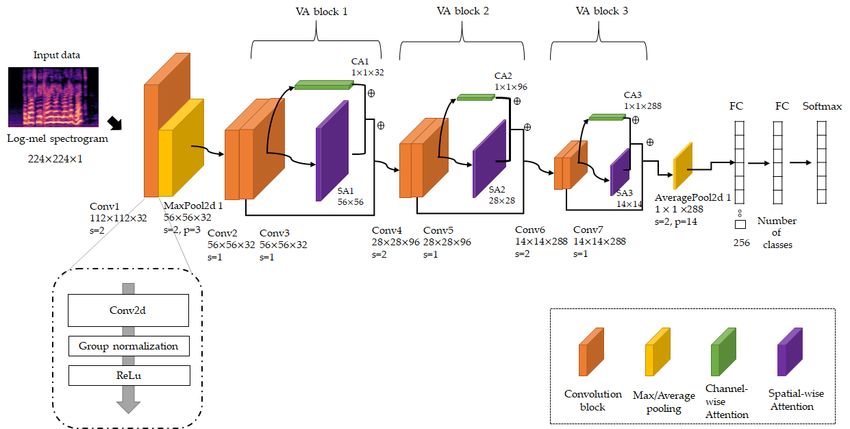
Sensors 2020, 20, 5559                                                                               2 of 21

have emerged in several domains, such as computer vision, speech recognition, and natural language
processing (NLP). Because deep-learning models can handle more complex features, recent SER
studies have used deep-learning models to identify speakers’ emotions using high-level features from
utterances. Many SER systems learn spectral features of utterances as high-level features, such as
gammatone, short-time Fourier transform (STFT), and mel-spectrogram, which are obtained as 2D
visual data by converting the time-based signal into the frequency domain utilizing the Fourier
transform and deep-learning models such as CNN and LSTM [12–15].
     The speech dataset has different acoustic features depending on the culture, context, and language
of the speakers. Therefore, the SER classification performance varies with speech datasets. However,
due to a lack of variety within speech datasets, it is difficult to classify the emotional state of speakers
in a new speech dataset that has not been learned. Therefore, recent studies have considered the
cross-corpus SER to classify emotions on a target speech dataset using a pretrained model on other
speech datasets. Numerous researchers have attempted to achieve improved cross-corpora accuracy.
Accordingly, transfer learning has primarily been adopted for cross-corpora.
     Transfer learning [16] is a machine-learning technique that aims to improve the performance
of a target domain with a small dataset by using knowledge from previously learned tasks with
large datasets. The underlying concept is to not only leverage the pretrained model’s weighted layer,
but also to selectively retrain some of the pretrained layers. In other words, some initial layers are
frozen to capture generic features of the pretrained domain, and the remaining layers are fine-tuned
to learn more specific features of the new domain. When the source dataset has a larger number of
training samples than the target dataset, the method of transferring and fine-tuning layers is effective in
assisting the learning target dataset. Speech datasets are composed of emotion-specific utterances with
different language, context, and recording times. Therefore, transfer learning is an effective method for
SER research when training small datasets utilizing the trained weights of large datasets.
     To achieve better performance in the speech dataset regardless of the utterance type, we propose
a method for identifying emotions by leveraging the previously trained weights in a large dataset.
In the proposed method, we use a log-mel spectrogram, which adopts mel scaling, which computes a
logarithmic scaling of the repetition frequency to represent human auditory characteristics representing
the 2D spectrogram to a spectrogram where the horizontal axis is the time, and the vertical axis is
the frequency of the speech signal and log-amplitude scaling to provide flexible and robust features.
We classify emotions using the log-mel spectrogram by learning the high-level neural features of
a spectrogram with a 2D CNN model and visual attention techniques. In our proposed visual
attention CNN (VACNN) model, by emphasizing the target-specific channels in the channel-wise
aspect and the most informative region of feature map in the spatial aspects through the visual attention
technique [17], the CNN model obtains more useful high-level information in the spectrogram for
improved emotion-classification performance.
     Our VACNN model is pretrained in a large dataset and is applied to fine-tune small datasets
for emotion classification. In addition, when learning small datasets, we utilize the bag of visual
words (BOVW) method [18] that represents each image by a histogram of the visual words to find
local and global features on the log-mel spectrogram to support the fine-tuned VACNN model.
In computer vision, feature descriptors (e.g., scale-invariant feature transform (SIFT), histogram of
oriented gradients (HOG), and speeded-up robust features (SURF)) are primarily used to detect
the edge and texture information of an image. The BOVW adapts the bag of words (BOW) method
used in NLP and implemented image features on the feature descriptor as the “words” of BOW.
The visual words represent local features in the image, and the BOVW creates a visual vocabulary by
grouping visual words based on their similarities. Because the BOVW represents a feature vector by
creating a sparse histogram, the BOVW is useful in capturing the local and global features in log-mel
spectrograms. Additionally, local and global features are expressed as attention weight through the
attention mechanism, so that the features learned by the convolution layer can be used to obtain local
and global information related to speech emotion in corpora. Moreover, methods that train spectral
Sensors 2020, 20, 5559 3 of 21
features using CNN for the source speech dataset and retraining for the target speech dataset have
never been used before in the SER task. This leads to reduced training times and enables improved
CNN model performance.
This study provides two key contributions:
(1) As a pretraining model, we train a log-mel spectrogram with a 2D CNN model with visual
attention modules. Visual attention consists of two modules: (1) A channel-wise attention module
that enhances convolutional features by the relationship between channels, so the model is able
to find informative features for feature refinement, and (2) a spatial attention module that assigns
weights to each pixel on convolutional features by concentrating spatial locations. Thus, the more
target-specific features are learned to improve the classification performance.
(2) We designed the VACNN model for pretraining a large speech dataset and fine-tuning a small
speech dataset to identify the emotion in utterances. Through fine-tuning, the proposed model
can consider the generic features of the pretrained layer and the specific features obtained
by retraining the pretrained layer. In addition, the textual information extracted from the
log-mel spectrogram through the feature descriptor is represented as a global statistic feature
and utilized as context attention weight in our VACNN to improve performance for SER and
cross-corpus SER. Our method exhibits a better overall accuracy of 7.73%, 15.12%, and 17.80%
for Ryerson Audio-Visual Database of Emotional Speech and Song (RAVDESS) [19], the Berlin
Database of Emotional Speech (EmoDB) [20], and Surrey Audio-Visual Expressed Emotion
(SAVEE) [21], respectively.
The remainder of the paper is organized as follows: In Section 2, we review existing SER literature.
In Section 3, we describe the steps of our proposed method. In Section 4, we describe our experimental
results and compare them with the state-of-the-art in the literature. Finally, in Section 5, conclusions
and future work are discussed.
2. Related Works
The SER field of research classifies the emotional state of a speaker by analyzing the digital signal
extracted from their utterances. In recent years, many researchers have conducted various studies
to classify emotions by analyzing various types of acoustic features extracted from speech signals.
Commonly, SER research uses a two-way method to analyze low-level features and utterance-based
spectral features.
Studies that use low-level features classify emotions by analyzing acoustic feature spaces, primarily
using SVM, GMM, HMM, and K-nearest neighbor (KNN). Sun et al. [9] applied decision tree SVM to
low-level features selected by the Fisher feature selection method in utterances. Then, they achieved
83.75% and 86.86% accuracy for the Chinese Emotional Speech Corpus (CASIA) [22] and the EmoDB
database, respectively. Kuchibhotla et al. [23] classified emotions through linear discriminant analysis,
regularized discriminant analysis (RDA), SVM, and KNN using low-level features selected using
feature subset selection techniques viz., sequential forward selection, and sequential floating forward
selection (SFFS). They achieved 92.6% accuracy for six emotions on EmoDB and 90.5% accuracy for six
emotions in the Spanish emotional speech database when they applied RDA to selected features using
the SFFS method. Noroozi et al. [24] selected 88 low-level features, including pitch, intensity, MFCC,
zero-crossing rate (ZCR), and filter bank energy parameters in utterances. Then, they used SVM or
random forest, with and without applying principal component analysis (PCA) to classify emotions in
utterances. They reported weighted accuracies of 56.07%, 65.28%, and 47.11% for SAVEE, Ryerson
Multimedia Laboratory (RML) [25], and eNTERFACE [26] datasets using Random Forest, respectively.
Fahad et al. [27] described a method to represent the discriminative features from MFCC through
a GMM and recognized emotions in utterances with HMM. They reported a weighted accuracy of
69.5% for the interactive emotional dyadic motion capture (IEMOCAP) databases [28]. In the studies
discussed above, they primarily learned low-level features using machine learning, and consideredSensors 2020, 20, 5559 4 of 21
only general acoustic features. This has the disadvantage of ignoring the relationship between features
that can be obtained from representations of utterances.
Other studies using spectral features, such as STFT and log-mel spectrograms, classify emotions
using deep-learning models. Misramadi et al. [29] combined bidirectional LSTM (BiLSTM) with
an attention mechanism to learn both the frame-wise raw spectral features and low-level features.
They attached a weighted pooling layer to the attention to compute the score for the contribution
of frames. They achieved weighted accuracy of 61.8% and 63.5% for IEMOCAP. Tao and Liu [30]
proposed a new variation of LSTM, advanced long short-term memory (A-LSTM), which applied a
weighted pooling Recurrent Neural Network (RNN) scheme. It could leverage the advantage of flexible
time dependency modeling capability. They applied A-LSTM to low-level features and sequential
acoustic features of IEMOCAP for SER and achieved an accuracy of 58.7%. Because they primarily
learn contextual information of sequence acoustic features using LSTM-based models, they could
ignore local correlations on the 2D spectral features depending on emotions.
Tarantino et al. [31] used the global windowing method on top of the already extracted frames to
express relationships between datapoints, and applied self-attention to extract 384 low-level features
to weight each frame based on correlations with the other frames. Then, they classified emotions using
a CNN model and achieved a weighted accuracy of 64.33% for IEMOCAP. In this work because they
applied windowing to an existing frame to overlap frames, frame related emotions could not receive a
weight score depending on which frame is overlapped by the global window.
Hararolasvadi and Demirel [32] selected the most discriminant frames using K-means clustering for
low-level features, including MFCC, pitch, intensity, and filter-bank energies. Later, for several frames,
they learned the spectra-temporal features from STFT through a 3D CNN model. They reported weighted
accuracies of 81.05%, 77.00%, and 72.33% for SAVEE for the six emotions, RML, and eNTERFACE’05
datasets, respectively. In this research, because the 3D CNN model learned only selected k frames,
the CNN model could ignore local correlations between spectral features on unselected frame
related emotions.
Mustaqeem and Kwon [33] revealed the amount of energy transmitted by a sound wave is
correlated to the amplitude of a sound wave. The amplitude of a sound wave denotes the maximum
displacement of an element in the middle from its rest location. They computed the maximum
amplitude in each frame using the peak value of sinusoidal wave function. The adaptive threshold
method [34] was used to remove the noises and silent portions, and, finally, a new audio file with the
same sample rates without any noise and silent signals was reconstructed. With this preprocessed audio,
they extracted STFT and used CNN and FC layers for SER. They achieved accuracies of 81.75% and
79.5% for IEMOCAP and RAVDESS, respectively. This method has a drawback in that the classifying
emotions can be time consuming because the audio file must be analyzed and converted to audio
without noise or silence for preprocessing. In the aforementioned studies [29–33], local correlations
between spectral features could be ignored by using normalized spectral features from pre-processing.
In recent years, cross-corpus SER studies have been performed to classify emotions for different
languages or genders. Schuller et al. [35] initially investigated cross-corpus SER studies using various
low-level features through an SVM. Zong et al. [36] designed a domain-adaptive least-squares regression
(DaLSR), which jointly trained the least-squares regression (LSR) model with the labeled training
samples from the source speech corpus. They achieved the best weighted accuracies of 52.27%,
36.40%, and 30.19% in EmoDB using eNTERFACE, eNTERFACE using EmoDB, and AFEW 4.0 using
EmoDB, respectively. Huang et al. [37] used a two-stage PCANet to cross-corpus SER. They train
feature extractors for source data, unlabeled target data, and generated intermediate data by PCANet
with filter alignment and fed output of three feature extractors as the final features into the source
data. They trained the source data with SVM and tested the target data. They achieved unweighted
accuracies of 61.41% and 63.75% for EmoDB using Airplane Behavior Corpus (ABC) [38], and ABC
using EmoDB, respectively. In these studies, they adopted unsupervised learning, so it could learn
irrelevant representations because of the absence of the label information.Sensors 2020, 20, 5559 5 of 21
Zhang et al. [39] designed transfer sparse discriminant subspace learning, which combines
discriminative subspace learning, graph-based distance metric, and feature selection. They achieved
an accuracy of 49.26%, 42.44%, and 42.42% for EmoDB using BAUM-1a, eNTERFACE using EmoDB,
and BAUM-1a [40] using EmoDB, respectively. Latif et al. [41] measured cross-corpus SER performance
using a low-level feature. They applied a deep belief network with three restricted Boltzmann machine
layers or sparse autoencoder and SVM to the source domain dataset and then applied transfer learning
for the target domain dataset. For positive or negative emotions, they learned acoustic features on FAU
Aibo [42] emotion corpus and IEMOCAP and then transferred these pretrained features when training
the EmoDB, SAVEE, and EMOVO corpus [43]. This research used captured feature distribution, so it
ignores the specific features of deep learning methods in which features of the source dataset are not
transferred to the training of the target dataset.
Liu et al. [44] designed a deep domain-adaptive convolutional neural network model, which
combined the CNN and domain-adaptive layer based on the maximum mean discrepancy (MMD)
regularization method. They learned salient features from the speech spectrograms and reduced the
distribution mismatch between the source and target datasets. They achieved an unweighted accuracy
of 49.93% and weighted accuracy of 58.13% for EmoDB using eNTERFACE, unweighted accuracy
38.10%, and weighted accuracy 38.10% for CASIA using EmoDB, and unweighted accuracy of 31.59%
and weighted accuracy of 31.68% for eNTERFACE using CASIA. This method uses MMD methods,
which can ignore class weight bias, so MMD can be minimized by either learning domain-invariant
representation or preserving the class weights in the source domain. In existing cross-corpus studies,
the discrepancy between feature distributions of different corpora have been considered. This can lead
to performance reduction because it ignores the target-specific features of spectral features. In order
to achieve better performance, we fused the fine-tuned our VACNN model pretrained on the source
dataset and the feature vector with the BOVW. It considers target-specific features of spectral features
and improves performance of cross-corpus SER. The proposed architecture and methodology in our
work are described in detail in next section.
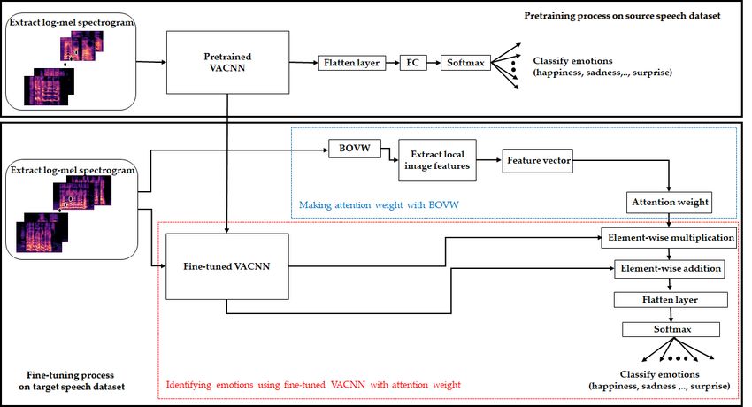
3. Proposed Methodology
In this study, to identify the emotions, we describe a model that learns the log-mel spectrogram on
a large dataset, and then propose a method that fine-tunes the pretrained model when learning a small
dataset. We use the characteristics of the log-mel spectrogram to recognize emotions in utterances.
Our method consists of two steps, as illustrated in Figure 1. First, we designed and pretrained our
VACNN model to a log-mel spectrogram extracted from the utterance of the large dataset (Figure 1,
top). The VACNN model is designed as a 2D CNN model that includes convolution blocks and a
spatial- and channel-wise visual attention module. The convolution block is composed of convolution
layers, group normalization (GN) [45], and rectified linear unit (ReLU) to learn high-level neural
features. In addition, both visual attention modules assist VACNN to capture the refined features
in the spatial- and channel-wise aspects. Second, we fused the fine-tuned VACNN model and the
attention weight of visual vocabulary for the log-mel spectrogram to identify the emotions for a small
dataset (Figure 1, bottom). We fine-tuned with the pretrained VACNN model on a large dataset in the
first step. To improve the fine-tuned VACNN, we extracted feature vectors from local image features
on a log-mel spectrogram using the BOVW and expressed it as an attention vector to assist VACNN.
For joint learning with feature vectors of BOVW, we computed the element-wise multiplication of the
attention vector and the fine-tuned VACNN. Then, we computed the element-wise sum to summarize
the features of high-level neural features in the VACNN and the feature vector with the BOVW. Finally,
a fully connected layer and softmax classifier were used to classify emotion in the log-mel spectrogram
on a small dataset. In the second step, we captured general and specific features using the fine-tuned
model (red block in the fine-tuning process), and utilized global static features represented by visual
vocabulary using the BOVW to capture the informational features in the target dataset (blue block in
the fine-tuning process).Sensors 2020, 20, 5559 6 of 21
Sensors 2020, 20, x FOR PEER REVIEW 6 of 21
Sensors 2020, 20, x FOR PEER REVIEW 6 of 21
Figure
Figure 1. 1. Overallarchitecture
Overall architectureofofour
ourpretraining
pretraining and
and fine-tuning
fine-tuning models
modelsfor
forSER.
SER.
Figure 1. Overall architecture of our pretraining and fine-tuning models for SER.
3.1.3.1. Visual
Visual Attention
Attention ConvolutionalNeural
Convolutional NeuralNetwork
Networkforfor Pretraining
Pretraining
3.1. Visual Attention Convolutional Neural Network for Pretraining
WeWe designed
designed a 2Da 2DCNNCNN modeltotocapture
model capturehigh-level
high-level neural
neural features
featuresof ofthe
thelog-mel
log-melspectrogram
spectrogram
Wesource
designed a 2DforCNN model to capture high-level neural features of the log-mel spectrogram
on the source dataset for SER. We used the log-mel spectrogram as a grayscale image shapewith
on the dataset SER. We used the log-mel spectrogram as a grayscale image shape with
on the source1 dataset
× 224 for SER. We andusedwidth
the log-mel spectrogram as achannels,
grayscalewhere
imageeachshape with
224224×224 ×1× as image
as the the image height
height and width size,
size, andandthethe numberof
number ofchannels, where each pixel
pixel has
has a
224 × 224 × 1 0astothe
a value image heightandandwhite
widthshading.
size, andTo theidentify
numberemotions
of channels, where eachour pixel has
value from from
adesigns
0 to 255
value from 0 to
for255
255
for and
black
for
black
black
white
and
shading.
white
To identify
shading. To
emotions
identify emotions
in utterances,
in utterances,
in
our model
utterances, our
model
designs
model
similar similar architecture
architecture to residualtoneural
residual neural (ResNet)
network network (ResNet) [46],
[46], which which
iswhich
mainly is mainly aused as a
designs
backbone similar
modelarchitecture
for vision to residual
recognition neural networkchannel
and designs (ResNet) [46],
and spatial-wiseis used
mainly asused
attention
backbone
as a
module
model for vision
backbone modelrecognition
for vision and designsand
recognition channel
designsandchannel
spatial-wise attention module
and spatial-wise attentioninspired
module by
inspired by convolutional block attention module (CBAM). The proposed VACNN model for the
convolutional
inspired by block attention
convolutional module
block (CBAM).
attention moduleThe(CBAM).
proposed VACNN
The proposed model
VACNNfor the source
model forspeech
the
source speech dataset is shown in Figure 2.
dataset
source is speech
showndataset
in Figure 2.
is shown in Figure 2.
Figure 2. Architecture of the proposed pretrain VACNN model.
Figure2.2.Architecture
Figure Architecture of
of the proposed
proposedpretrain
pretrainVACNN
VACNNmodel.
model.Sensors 2020, 20, 5559 7 of 21
We first obtained 112 × 112 feature maps, which have high-level features extracted from 3 × 3
convolution layers (stride = 2), which have 32 filters. To obtain the fine-grained features, we also applied
GN and ReLU after the convolution layer. We identified the three processes (convolution-GN-ReLU)
as a convolution block. The GN is inspired by layer normalization that normalizes along the channel
dimension, and instance normalization that normalizes each sample. To utilize the advantage that
the computations of layer and instance normalization are independent of batch size, GN divides the
channels into groups and computes normalization. We denoted the number of groups G and the
number of channels C. After the convolution layer, GN decides the number of channels per group
as C/G. For C/G, GN uses a feature-normalization method, such as batch normalization along the
height and width axes. Because GN’s computation is dependent on batch size, GN can show stable
performance in a wide range of batch sizes. Therefore, we used GN to normalize the feature maps with
high-level features on a log-mel spectrogram, such that the model can be normalized stably, regardless
of the small batch size according to the number of training samples. In addition, we applied the ReLU
function to activate the model. Then, we downsampled the content of feature maps to 56 × 56 by using
3 × 3 max pooling (stride = 2) to reduce the execution time while maintaining their salient features.
Next, we designed three VA-blocks to sequentially learn high-level neural features. Each VA block
has two convolution blocks as a first step. The convolution block is composed of 3 × 3 convolution layers,
GN, and ReLU activation, but shows a difference in stride size. In the first VA block, both convolution
blocks use a 1 × 1 stride with a convolution layer, which is convolved with the input at every pixel with
overlapping receptive fields, resulting in a 56 × 56 × 32 refined feature map. Otherwise, the second
uses a 2 × 2 stride with convolution layers in the first convolution block to capture high-level neural
features with a downsampled feature map of 28 × 28 × 96, using a 1 × 1 stride with convolution
layers in the second convolution block to find cross-channel correlations. The third VA block uses
two convolution blocks with the same structure as the second VA block with 288 filters and obtains
14 × 14 × 288 refined feature maps. Each convolution block in the VA blocks has a normalized layer
by GN and is activated by ReLU. In this model, we used 3 × 3 filters with convolution layers to learn
local features with a small receptive field proven by ResNet and VGG, and incrementally increase the
number of filters of the same size to extract the high-level neural features from spectrograms. Thus,
we employed the number of filters for convolutional layers, which resulted in the best performance on
the validation set.
After the last convolution block of VA blocks, we applied channel-wise visual attention and spatial
visual attention modules to obtain fine-grained features. We concatenated the VA blocks by adding
convolutional features. However, we subsequently performed spatial and channel-wise attention for
features captured from convolution blocks, so that features can determine where to focus and what
is meaningful on feature maps. These modules assist the model in learning target-specific features
of spatial and channel-wise aspects by passing the fine-grained feature from an earlier VA block to a
later VA block. Our VA modules were inspired by the CBAM by Woo et al. [47]. They jointly exploit
the inter-channel relationship initially investigated by Hu et al. [48] and the inter-spatial relationship
initially investigated by Zagoruyko and Komodakis [49]. High recognition performance in object
detection research is obtained with CBAM by exploiting the inter-channel relationship of features,
and then exploiting the inter-spatial relationship of the channel-wise refined feature. Our VA module
is similar to CBAM, but we devised a suitable VA module to refine the high-level neural features.
We denoted the height of the feature map as H, and the width of the feature map as W. The channel-wise
refined features Fc ∈ R1 × 1 × C from the channel-wise attention module are represented to emphasize
the informative features according to the channel relationship in the learned feature map V ∈ RH × W × C ,
as follows:
Fc = σ(W1 (W0 (GAP(V ))) + W1 (W0 (GMP(V )))). (1)
Here, σ is the sigmoid activation. W0 ∈ R1 × 1 × C/r and W1 ∈ R1 × 1 × C are parameters with a
multi-layer perceptron (MLP) layer, where r is the reduction ratio for the squeeze layer to emphasize
the informative feature between channels.Sensors 2020, 20, 5559 8 of 21
Our channel-wise attention module squeezes and restores the number of filters to aggregate and
emphasize inter-channel relationships in feature maps and applies sigmoid activation to parameterize
squeezed weight around the non-linearity. In [47,48,50], it is reported that the bottleneck configuration
with two FC layers, which reduces and restores the number of filters, is useful to emphasize channel-wise
dependencies. Sigmoid functions are inherently non-linear and thus the neural networks, perform
channel-wise recalibration by multiplying a value between 0 and 1 for each channel of the feature maps.
In addition, we applied global average pooling (GAP) and global max pooling (GMP) to generate
channel descriptors that include static information in feature maps. Woo et al. argued that max-pooling
and average pooling which are useful for obtaining channel-wise refined features. Max-pooling
encodes the degree of the most salient part, whereas average pooling encodes global features to the
channel. However, in previous studies [51,52], because GAP aggregates channel-wise statistics of
each feature map into one feature map, it forces the feature map to recognize certain elements within
the spectral features related target class. Additionally, GAP reduces overfitting because there are no
parameters to be learned in the global average pooling layer, reported in [51]. The GMP focuses on a
highly localized area on spectral features to find interpretable features within feature maps. The GMP’s
advantage with localized features is aligned with previous research [53,54]. Therefore, we argue that
it is useful for GAP, which represents the global feature of all channels and GMP, which extracts the
most specific portion of all channels to refine deep spectral features in the channel axis in learning SER
spectral features.
Next, we utilized our spatial attention module to find the inter-spatial relationship in the feature
map. Spatial attention encodes the spatial area of features by aggregating the local feature at spatial
position to capture inter-spatial relationship [17]. Spatial attention is commonly constructed by
computing statistics across the channel dimension. We obtained a spatially refined feature map
Fs ∈ RH × W as follows:
Fs = σ conv71 × 7 [AvgPool(V ); MaxPool(V )] . (2)
Here, σ is the sigmoid activation. conv71 × 7 denotes a 7 × 7 convolution operation with 1 × 1
stride, aggregating high-level features to a feature map having one channel. AvgPool is the average
operation of values across the channel dimension, MaxPool, and is the maximum operation of values
across channel dimensions.
For the feature map V from the convolution layer, we computed the average and max pooling
operations across the channel axis. Then, we concatenated the average and maximum-pooled
features and apply a convolution layer. These processes are similar to CBAM, but the convolution
layer is different. The CBAM adopts a standard 7 × 7 convolution layer, but we used unbiased
7 × 7 convolution with a 1 × 1 stride and activated refined features using sigmoid. Because the
convolution layer calculates spatial attention, we used an unbiased convolution layer to reduce the
risk of model overfitting due to bias that diversifies the model computation. In addition, we set
the number of channels to one to aggregate and regularize the spatial information on average- and
max-pooled features.
The CBAM applies the spatial attention module to a channel-wise refined feature and adopts
sigmoid activation, which is argued to show better performance. However, we applied the spatial
attention module and channel-wise attention module separately. By separately extracting the spatial
and channel relationship information in the feature map extracted from the convolution block,
the relationship of the original characteristic can be more widely detected. In addition, we computed
the element-wise sum of spatial refined features and channel-refined features to reduce information
transformation for learning high-level neural features.
The features from the third VA block with the convolution block and both spatial and channel-wise
attention modules were normalized in group normalization and ReLU activation. In addition, we obtained
an average pooled feature map with 1 × 1 × 288, calculating the average for feature maps. The average
pooled feature map enters a fully connected (FC) layer with 256 neurons, limiting redundancy and the
softmax classifier identifies emotions using the log-mel spectrogram.Sensors 2020, 20, 5559 9 of 21
This
Sensors 2020,model was
20, x FOR previously
PEER REVIEW trained with large datasets such as Toronto Emotional Speech Set
9 of 21
(TESS) [55] and the Ryerson Audio-Visual Database of Emotional Speech and Song (RAVDESS) for
detecting emotions
detecting emotions in in log-mel
log-mel spectrograms.
spectrograms. The model architecture
The model architecture and
and pretrained
pretrained weights
weights are
are
transferred to the learning process of the target datasets. In the next section, we describe the
transferred to the learning process of the target datasets. In the next section, we describe the method method
of leveraging
of leveraging the the pretrained
pretrained model
model and
and visual
visual vocabulary
vocabulary with
with the
the BOVW
BOVW when
when learning
learning other
other
speech datasets.
speech datasets.
3.2. Fusing Fine-Tuned
3.2. Fine-Tuned Model
Model and
and Attention
AttentionWeight
Weightwith
withBag
BagofofVisual
VisualWords
Words
In this
In this section,
section, we we describe
describe the
the fine-tuning
fine-tuning method
method to to learn
learn high-level
high-level features
features ofof small
small datasets
datasets
using pretrained layers
using layers forfor aalarge
largedataset.
dataset.Transfer
Transfer learning
learning shows
shows better performance
better performance to freeze the
to freeze
initial
the several
initial layers
several and fine-tuned
layers other other
and fine-tuned layers layers
when the when target
thedomain dataset is
target domain different
dataset from the
is different
source
from thedomain
source dataset
domainand has and
dataset fewer training
has samples samples
fewer training than thethan
sourced domain domain
the sourced dataset. dataset.
Speech
datasetsdatasets
Speech have a have
closea relationship, including
close relationship, emotions,
including but they
emotions, havehave
but they different features
different featuressuch as
such
language,
as language, intensity,
intensity, andandspeed. Therefore,
speed. Therefore,when whentaking the the
taking pretrained
pretrainedlayers on aonlarge
layers dataset,
a large we
dataset,
freeze
we layers
freeze up to
layers upthe to first VA block
the first VA blockand unfreeze
and unfreeze and retrain other other
and retrain layers.layers.
In the fine-tuning model,
In the fine-tuning
we downsampled
model, we downsampled featurefeature to 7 to
mapsmaps × 77 ×with 2 ×2 2× average
7 with 2 averagepooling
poolingtotoaggregate
aggregate feature maps
feature maps
while preserving the localization of high-level neural features. Furthermore,
while preserving the localization of high-level neural features. Furthermore, we reshaped feature maps we reshaped feature
maps
to 49 ×to288 × 288
49 to to jointly
jointly learn feature
learn feature vectorsvectors
from the from
BOVWthe BOVW
and to and
adaptto to
adapt
the FCto the FC layer.
layer.
In addition,
In addition, to to learn
learn specific
specific features
features ofof the
the target
target dataset,
dataset, wewe jointly
jointly learned
learned thethe feature
feature vector
vector
extractedby
extracted byanalyzing
analyzing thethe log-mel
log-mel spectrogram
spectrogram throughthrough
the BOVW the BOVW and fine-tuned
and fine-tuned model. The model. The
proposed
proposed fine-tuned
fine-tuned model is shown modelinisFigure
shown3.in Figure 3.
Figure 3. Architecture of the proposed fine-tuned model.
Figure 3. Architecture of the proposed fine-tuned model.
We ensemble the BOVW and fine-tuned models to improve classification performance by
learning features of both feature vectors expressing which part of the log-mel spectrogram primarilySensors 2020, 20, 5559 10 of 21
We ensemble the BOVW and fine-tuned models to improve classification performance by learning
features of both feature vectors expressing which part of the log-mel spectrogram primarily appears
according to emotion and high-level neural features learned by the VACNN model. The BOW is a
feature extraction technique primarily used in NLP and represents each sentence or document as a
feature vector with each word by counting the number of times each word appears in a document.
The BOW model is also applicable for vision-recognition research as BOVW. We use the BOVW to
represent the features of the log-mel spectrogram in three steps. First, we extracted local features
from images using the KAZE descriptor, which is robust to rotation, scale, and limited affine. Then,
we divided the feature space through a clustering algorithm as K-means clustering and defined the
center point of each group as a visual word. In this step, we used the silhouette value, which measures
how similar a point is to its own cluster compared to other clusters. In previous studies [56,57],
it is reported that silhouette achieves the best result in most case. In addition, [57] reported that the
silhouette shows most robust performance among cluster validity indices in their research. Given
observation p, let dsp be the average dissimilarity between the data point and all other points in its
own cluster. Let dop be the lowest average dissimilarity between data points and all data points in
another cluster. The silhouette Silp for each data point p is computed as follows:
dop − dsp
Silp = . (3)
max dsp , dop
We computed the average for the silhouette value to range from −1 to 1; an average silhouette
value close to 1 indicates that the point is correctly placed. We computed the average silhouette value
for visual words, and then selected the largest number of clusters that show a high silhouette value.
Finally, we created histograms with 128 visual words as feature vectors to represent the features
of the log-mel spectrogram. We employed the number of visual words that resulted in the best
performance on the validation set. The feature vector is entered into the MLP layer with 49 neurons to
squeeze the information of the feature vector. We expanded the dimensions and entered the MLP layer
with 288 neurons to assist the fine-tuned model.
In addition, we applied context attention to assist the fine-tuned model to jointly learn the
refined feature vector. Whereas the aforementioned visual attention emphasizes the salient features
on the feature map learned by the convolution layer, context attention compresses all the necessary
information of sequence data into a fixed-length vector in a different manner with visual attention. In
our implementation, the attention vectors are computed and applied to features extracted from the
VACNN, as follows:
SCts = ht | ·Whs , (4)
exp(SCts )
αts = Pn , (5)
i=1 exp(SCi )
X
Ct = αts ·hs , (6)
s
avt = tanh(Wc [Ct ; ht ]), (7)
av f s = tanh(Oavt ) + hs . (8)
Here, ht denotes the last hidden state of the refined feature vector for the target sequence, denotes
the dot product, and hs denotes all hidden states of the refined feature vector for the input sequence.
i denotes the index of hidden states, n denotes the number of hidden states, and denotes concatenate.
Wc is a learnable parameter with an MLP. In addition, O is extracted features using the VACNN model.
We utilize all the hidden states of the refined feature vector hs to calculate scores SCts using Luong’s
multiplicative style [58], which generalizes all the hidden states with unbiased MLP and dot product
to the last hidden state to compare their similarity. Then, we employed softmax on these scores to
produce the attention weights αts as a probabilistic interpretation to which state i is to be paid or to beSensors 2020, 20, 5559 11 of 21
ignored. The context vector Ct is generated by performing an element-wise multiplication of αts with
each state of hs . The context vector is generated using the sum of the hidden states weighted by the
attention weight. We can attain an attention vector avt by applying a hyperbolic tangent (tanh) for the
concatenated context vector Ct and the last hidden state ht . For joint learning with feature vectors,
we fed the attention vector avt into feature maps F of the VACNN using element-wise multiplication,
and used tanh as the nonlinear activation. Then, we can attain summarized features av f s by computing
the element-wise sum with hs to enforce efficiency of learning salient features in both high-level neural
features in the VACNN and the feature vector with the BOVW. We applied ReLU activations av f s and
then classified emotions using a classification layer and a softmax classifier with output classes.
4. Results and Discussion
4.1. Dataset
4.1.1. Berlin Database of Emotional Speech
The EmoDB [20], a benchmark dataset, is a Berlin emotional speech database produced by
Burkhardt. The EmoDB covers the following seven emotion categories: anger, boredom, neutral,
disgust, fear, happiness, and sadness. The voice was recorded by five male and five female actors
between the ages of 20 and 30. The speech corpus consists of 10-sentence German phrases with different
lengths, and the total number of utterance files is 535.
4.1.2. Ryerson Audio-Visual Database of Emotional Speech and Song
RAVDESS [19], a benchmark dataset, is a multimodal database used to recognize emotions with
facial expression and voice data (speech, song). It primarily includes three categories: voice-only,
face-and-voice, and face-only. Speeches were recorded with eight emotions—neutral, calm, happiness,
sadness, anger, fear, surprise, and disgust, by 24 professional actors consisting of 12 women and
12 men. Additionally, each speech was recorded separately with strong intensity and normal intensity
to express aspects of the voice based on the degree of emotion. We use voice-only data with 1440
utterance files to classify emotions using only utterances.
4.1.3. Toronto Emotional Speech Set
TESS [55], a benchmark dataset, is an English emotional speech database recorded by two female
actors recruited from the Toronto area. It has seven emotions: anger, disgust, fear, happiness, pleasant
surprise, sadness, and neutral. The female actors, aged 26 and 64 years, spoke a set of 200 target words
for each of the seven emotions as well as with the carrier phrase “say the word.” Thus, the speech
dataset consisted of a total of 2800 files with 400 sentences recorded for each emotion.
4.1.4. Surrey Audio-Visual Expressed Emotion
SAVEE [21], a benchmark dataset, is a multimodal database used to recognize emotions with
facial expressions and audio speech datasets. It is recorded by four male actors, aged between 27 and
31. Speech is recorded as seven emotions related to anger, disgust, fear, happiness, sadness, surprise,
and neutral. It has a speech data set of 480 sentences. Because we aim to identify the emotion of the
speaker, we use only the speech dataset. Table 1 shows an overview of each speech dataset used.Sensors 2020, 20, 5559 12 of 21
Table 1. Overview of the selected datasets.
Dataset Language Utterances Emotions Emotion Labels
Anger, Boredom, Neutral, Disgust, Fear,
EmoDB German 565 7
Happiness, Sadness
Neutral, Calm, Happiness, Sadness, Anger,
RAVDESS English 1440 8
Fear, Surprise, Disgust
Anger, Disgust, Fear, Happiness, Pleasant
TESS English 2800 7
Surprise, Sadness, Neutral
Anger, Disgust, Fear, Happiness, Sadness,
SAVEE English 480 7
Surprise, Neutral
4.2. Experiments
We propose a CNN-based model with spatial and channel-wise visual attention modules to
identify emotions in utterances and learn large speech datasets as prework. In addition, we propose a
fine-tuning method to improve the performance of classification for speech datasets using a pretrained
model and feature vector extracted by the BOVW. To verify the performance of our proposed method,
we first selected a large dataset to create a pretrained model. The TESS dataset has the largest number
of audio files among the four speech datasets in EmoDB, RAVDESS, SAVEE, and TESS. However,
because TESS is recorded by only two speakers, overfitting is a concern in experiments. Therefore,
we used both TESS, which has two speakers and RAVDESS, which has 24 speakers for the pretraining
dataset. To verify the performance of SER and cross-corpus SER, we tested for EmoDB, SAVEE,
and RAVDESS separately.
The log-mel spectrogram has been shown to effectively distinguish features in SER through SER
research. When extracting the log-mel spectrogram in utterances, the fast Fourier transformation
window length is 2048 and the hop length is 512. For training in our model, the log-mel spectrogram is
represented as a 2D grayscale image with 224 × 224 pixels.
For each experiment, we divided the data such that 80% was used for training and 20% for
testing. We performed 5-fold cross-validation. In 5-fold cross validation, each fold was iteratively
selected to test the model, and the remaining four folds were used to train the model [59,60]. For group
normalization, we fix the number of groups to 8. Also, for channel-wise attention in our VA module,
we fix the reduction ratio to 4. We use a batch size of 8, and the cross-entropy criterion is used as the
training objective function. The Adam algorithm is adopted for optimization. A group normalization
layer is adopted in VACNN to avoid overfitting. The model was trained with a 0.001 learning rate
and a decay one later every 10 epochs. To avoid overfitting, we used l2 weight regularization with
factor 0.0001.
To avoid overfitting, we adopted regularization methods in the experiments. First, early stopping
is used to train the model to prevent over-fitting. Overfitting occurs when the learning degree is
excessive, and underfitting occurs when the learning degree is poor. Early stopping is a continuously
monitored error during training through early stopping. When performance on the validation dataset
starts to decrease it stops model training before it overfits the training dataset. Thus, it can reduce
overfitting and improve the model generalization performance.
As another method to prevent overfitting, model selection was used in our experiments. Model
selection is a method that selects a model from a group of candidate models. Model selection designated
the most predictive and fitted model based on the validation accuracy for SER.
4.2.1. Results and Performance of VACNN for Pretraining
We used the VACNN architecture to train the TESS and RAVDESS datasets for pretraining. To train
the two datasets simultaneously, the speech data label was set as anger, disgust, fear, happiness, surprise,
sadness, and neutral. The batch size is 8 in the whole training process. The cross-entropy criterion was
used as the training objective function. The Adam algorithm was adopted for optimization. A group
normalization layer is adopted in the VACNN to avoid overfitting. First, we validate the TESS andSensors 2020, 20, 5559 13 of 21
RAVDESS datasets using the VACNN model for pretraining. To match the label with TESS, the calm
label of RAVDESS was recognized as a neutral emotion for pretraining. Table 1 shows the performance,
class level precision, recall, F1-score, and overall accuracy tested in TESS and RAVDESS using the
VACNN. Precision refers to the percentage of results that are relevant. Recall refers to the percentage
of total relevant results correctly classified by the algorithm. The F1-score is a statistical feature defined
as the harmonic mean between precision and recall. The overall accuracy is calculated by summing
the number of correctly classified values and dividing by the total number of values.
Table 2 enumerates the performance of the proposed VACNN model over the TESS and RAVDESS,
which indicates the effectiveness of the model in recognizing emotions with an overall accuracy of
89.03%. In precision, all emotions are recognized with more than 80% class accuracy. Anger showed
the highest accuracy of 94%. Fear and surprise showed the highest accuracy of 94%, whereas happiness
showed the lowest accuracy of 75%.
Table 2. Confusion matrix based on TESS and RAVDESS dataset for pretraining.
Emo Class Precision Recall F1-Score
Anger 0.94 0.88 0.91
Disgust 0.89 0.92 0.90
Fear 0.83 0.94 0.88
Happiness 0.90 0.75 0.82
Neutral 0.92 0.89 0.91
Sadness 0.83 0.90 0.87
Surprise 0.93 0.94 0.93
Average 0.89 0.89 0.89
4.2.2. Results and Performance of Cross-Corpus SER Test with Fine-Tuned VACNN and BOVW
To test the cross-corpus SER performance, we use the pretrained VACNN with TESS and
RAVDESS and apply it to learning the target dataset. When learning the target dataset, we freeze the
pretrained weight to the first VA block, retrain layers up to the last average pooling operation in the
VACNN architecture, and jointly learn the feature vector extracted by the BOVW through a context
attention mechanism. We tested cross-corpus SER performance for SAVEE, RAVDESS, and EmoDB.
For fine-tuning process, we recognized emotions for RAVDESS with eight emotions. Table 3 presents
the overall accuracy performance of the VACNN + BOVW with and without fine-tuning. In addition,
Table 3 shows that the overall accuracy performance of the model has the same structure as the
fine-tuned VACNN structure, but the CBAM module is applied instead of our VA module to compare
the performance of the VA and CBAM modules.
Table 3. Comparison of overall accuracy using the proposed VACNN + BOVW, fine-tuned VACNN +
BOVW, and fine-tuned VACNN with CBAM instead VA module + BOVW.
Fine-Tuned VACNN + Fine-Tuned VACNN
Dataset Pure VACNN + BOVW
BOVW (CBAM) + BOVW
RAVDESS 0.72 0.83 0.77
EmoDB 0.77 0.87 0.81
SAVEE 0.69 0.75 0.72
For each dataset, the transferred VACNN + BOVW with a pretrained layer on the other dataset
showed higher accuracy than the purely trained VACNN + BOVW. In addition, our fine-tuned model
shows a higher performance than the VACNN using CBAM instead of the VA module.
Tables 4–6 represent the SER performance in terms of precision, recall, and F1-score for the tested
RAVDESS, EmoDB, and SAVEE datasets, respectively, for pretraining with TESS and RAVDESS.Sensors 2020, 20, 5559 14 of 21
Table 4. Cross-corpus emotion recognition result using proposed fine-tuning method on RAVDESS.
Emo Class Precision Recall F1-Score
Anger 0.77 0.91 0.83
Calm 0.95 0.89 0.92
Disgust 0.89 0.85 0.87
Fear 0.91 0.84 0.87
Happiness 0.81 0.74 0.77
Neutral 0.74 0.88 0.80
Sadness 0.74 0.76 0.75
Surprise 0.86 0.86 0.85
Average 0.83 0.83 0.83
Table 5. Cross-corpus emotion recognition result using proposed fine-tuning method on EmoDB.
Emo Class Precision Recall F1-Score
Anger 0.94 0.91 0.93
Boredom 0.87 0.87 0.88
Disgust 0.95 0.95 0.97
Fear 0.74 0.80 0.77
Happiness 0.86 0.73 0.79
Neutral 0.80 0.85 0.81
Sadness 0.86 0.96 0.91
Average 0.86 0.87 0.87
Table 6. Cross-corpus emotion recognition result using proposed fine-tuning method on SAVEE.
Emo Class Precision Recall F1-Score
Anger 0.74 0.58 0.65
Disgust 0.81 0.65 0.72
Fear 0.59 0.76 0.67
Happiness 0.72 0.59 0.65
Neutral 0.88 0.93 0.90
Sadness 0.73 0.83 0.78
Surprise 0.59 0.65 0.67
Average 0.72 0.71 0.72
Table 4 shows the precision, recall, and F1-score for eight emotions for RAVDESS. Our method
shows an overall accuracy of 83.33% for RAVDESS. In terms of precision, calm emotion showed 95%
highest accuracy in the eight emotions, whereas sadness and neutral emotion showed 74% accuracy.
In recall, anger showed the highest accuracy of 91%, whereas happiness showed the lowest accuracy
of 74%.
Table 5 shows the precision, recall, and F1-score for seven emotions for EmoDB. Our method
shows an overall accuracy of 86.92% for EmoDB. In precision, disgust registered at 95% and had the
highest accuracy, whereas fear showed the lowest accuracy of 74%. In recall, sadness showed the
highest accuracy of 96%, whereas happiness showed the lowest accuracy of 73%.
Table 6 shows the precision, recall, and F1-score for seven emotions for SAVEE. Our method
shows an overall accuracy of 75% for SAVEE. In terms of precision, neutral emotion achieved 88%
and had the highest accuracy in the seven emotions, whereas surprise showed the lowest accuracy of
59%. In recall, neutral emotions showed the highest accuracy of 93%, while anger showed the lowest
accuracy of 58%.
Tables 7–9 show the confusion matrix in RAVDESS, EmoDB, and SAVEE, respectively, for the
cross-corpus SER test.Sensors 2020, 20, 5559 15 of 21
Table 7. Confusion matrix for emotion prediction on RAVDESS using RAVDESS and TESS.
Emo Class Anger Calm Disgust Fear Happiness Neutral Sadness Surprised
Anger 0.91 0.00 0.03 0.00 0.03 0.00 0.00 0.03
Calm 0.00 0.89 0.00 0.00 0.05 0.02 0.05 0.00
Disgust 0.10 0.02 0.85 0.00 0.00 0.00 0.03 0.00
Fear 0.00 0.00 0.03 0.84 0.03 0.00 0.08 0.02
Happiness 0.07 0.00 0.02 0.04 0.74 0.02 0.04 0.07
Neutral 0.00 0.00 0.00 0.00 0.12 0.88 0.00 0.00
Sadness 0.05 0.03 0.03 0.03 0.03 0.08 0.76 0.00
Surprise 0.00 0.00 0.00 0.06 0.02 0.00 0.06 0.86
Table 8. Confusion matrix for emotion prediction on EmoDB using RAVDESS and TESS.
Emo Class Anger Boredom Disgust Fear Happiness Neutral Sadness
Anger 0.91 0.00 0.00 0.04 0.05 0.00 0.00
Boredom 0.00 0.87 0.00 0.00 0.00 0.10 0.03
Disgust 0.00 0.00 0.95 0.05 0.00 0.00 0.00
Fear 0.04 0.00 0.00 0.8 0.00 0.04 0.12
Happiness 0.00 0.00 0.04 0.15 0.73 0.08 0.00
Neutral 0.03 0.12 0.00 0.00 0.00 0.85 0.00
Sadness 0.00 0.00 0.00 0.00 0.00 0.04 0.96
Table 9. Confusion matrix for emotion prediction on SAVEE using RAVDESS and TESS.
Emo Class Anger Disgust Fear Happiness Neutral Sadness Surprised
Anger 0.58 0.08 0.08 0.13 0.00 0.00 0.13
Disgust 0.00 0.65 0.07 0.00 0.12 0.08 0.08
Fear 0.00 0.05 0.76 0.05 0.05 0.05 0.05
Happiness 0.22 0.00 0.05 0.59 0.00 0.00 0.14
Neutral 0.00 0.00 0.00 0.00 0.93 0.07 0.00
Sadness 0.00 0.04 0.00 0.00 0.13 0.83 0.00
Surprise 0.00 0.3 0.05 0.00 0.00 0.00 0.65
In Table 7, RAVDESS shows the highest performance in anger, and anger is confused with
disgust, happiness, and surprise. In addition, sadness shows the lowest accuracy and is confused with
neutral emotions.
In Table 8, EmoDB shows the highest accuracy with disgust, and disgust is confused with fear.
In addition, happiness shows the lowest accuracy and is confused with neutral and disgust.
In Table 9, SAVEE showed the highest accuracy in neutral, and neutral was confused with sadness.
Anger showed the lowest accuracy and confused surprised and happiness.
As interest in cross-corpus SER increased, we proposed pretraining on a large dataset with TESS
and RAVDESS and a fine-tuned model when learning a relatively small dataset with RAVDESS,
EmoDB, and SAVEE. Table 10 compares the performance with cross-corpus SER studies in SAVEE,
EmoDB, and RAVDESS, respectively. Latif et al. used latent codes extracted by 88 low-level features
related to spectral energy, frequency, cepstral features, and dynamic information based on a generative
adversarial network (GAN). They pretrained the source dataset with SVM and transferred the feature
space to the target dataset. Mao et al. [61] pretrained the local invariant feature extracted by a sparse
autoencoder on the raw spectrogram with SVM for the source dataset and transferred feature space
with SVM to identify emotions on the target dataset. Goel and Beigi [62] extracted 384 features related
to ZCR, root-mean-square energy, pitch, and pretrained source dataset with LSTM and a fine-tuned
model to learn the low-level features of the target dataset. Mustaqeem and Kwon designed a stride
deep CNN model and learned the high-level features on a raw spectrogram and tested it in the
target dataset. It was shown that there have been many studies on cross-corpus SER performance,
mainly transferring the feature space or fine-tuned high-level features. Milner et al. [63] extractedYou can also read