THE PLASMA ENVIRONMENT OF COMET 67P/CHURYUMOV-GERASIMENKO THROUGHOUT THE ROSETTA MAIN MISSION
←
→
Page content transcription
If your browser does not render page correctly, please read the page content below

THE PLASMA ENVIRONMENT OF COMET
             67P/CHURYUMOV-GERASIMENKO THROUGHOUT
                      THE ROSETTA MAIN MISSION

   K. C. HANSEN1,∗ , T. BAGDONAT2 , U. MOTSCHMANN2 , C. ALEXANDER3 ,
M. R. COMBI1 , T. E. CRAVENS4 , T. I. GOMBOSI1 , Y.-D. JIA1 and I. P. ROBERTSON4
                    1 Department     of Atmospheric, Oceanic and Space Sciences,
                      University of Michigan, Ann Arbor, Michigan, 48109, USA
2 Institute for Theoretical Physics, Technical University of Braunschweig, Braunschweig, Germany
                   3 Jet Propulsion Laboratory, Pasadena, California, 91109, USA
   4 Department of Physics and Astronomy, University of Kansas, Lawrence, Kansas, 66045, USA

                      (∗ Author for correspondence: E-mail: kenhan@umich.edu)

              (Received 30 August 2006; Accepted in final form: 12 December 2006)

Abstract. The plasma environment of comet 67P/Churyumov-Gerasimenko, the Rosetta mission
target comet, is explored over a range of heliocentric distances throughout the mission: 3.25 AU
(Rosetta instruments on), 2.7 AU (Lander down), 2.0 AU, and 1.3 AU (perihelion). Because of
the large range of gas production rates, we have used both a fluid-based magnetohydrodynamic
(MHD) model as well as a semi-kinetic hybrid particle model to study the plasma distribution. We
describe the variation in plasma environs over the mission as well as the differences between the
two modeling approaches under different conditions. In addition, we present results from a field
aligned, two-stream transport electron model of the suprathermal electron flux when the comet is near
perihelion.

Keywords: comet, Churyumov-Gerasimenko, plasma, hybrid simulation, MHD simulation

                                       1. Introduction

The Rosetta mission target, Comet 67P/Churyumov-Gerasimenko (hereafter re-
ferred to as 67P/CG), is a fairly typical Jupiter-Family comet with a perihelion
distance of 1.3 AU and a maximum expected gas production rate in the vicinity of
5 × 1027 s−1 . Most of our knowledge of the plasma environment of comets comes
from ground-based observations of the ion tails of bright comets and the several
flybys of both weak and bright comets: 21P/Giacobini-Zinner by the ICE satellite
in 1985, 1P/Halley by several spacecraft in 1986, 26P/Grigg-Skjellerup by Giotto
in 1992 and 19P/Borrelly by Deep Space 1 in 2001. While there has been some
modeling work of the weaker comets, most of the published work is on Halley
activity class comets at heliocentric distances near 1 AU and gas production rates
of several ×1029 molecules s−1 .
   A well-developed cometary atmosphere extends to distances orders of mag-
nitude larger than the size of the nucleus. Self-consistent models of cometary
Space Science Reviews (2007) 128: 133–166
DOI: 10.1007/s11214-006-9142-6
                                                                                   C   Springer 2007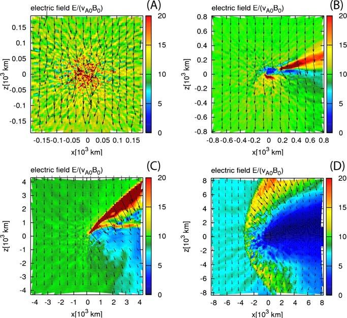
134                              K. C. HANSEN ET AL.

atmospheres must describe phenomena taking place at spatial and temporal scales
ranging from the initiation of transonic dusty gas flow near the nucleus (typical
scale lengths of 10−2 –10−1 km) to fast chemical reactions (typical scales of 100 –
102 km) to the formation of the cometary ionosphere (typical scales of 103 –104
km), to the solar wind interaction of the cometary atmosphere (typical scales of
105 –107 km). This range of phenomena and length scales is challenging and has
not been comprehensively modeled for any comet. This paper has been produced
as part of an effort to develop a systematic, comprehensive and self-consistently
coupled model of the environment of 67P/CG. Although this paper concentrates
on only the plasma environment of the comet, the models we present are being
coupled together with nucleus, Knudsen-layer, dust and gas models as part of an
International Space Science Institute (ISSI) project.
    The main photoionization product in the cometary coma is H2 O+ . These wa-
ter ions transfer a proton to other neutral molecules, which have a higher proton
affinity than the OH radical (the prime example is H2 O+ + H2 O → H3 O+ + OH).
The proton affinity of the parent molecules determines the reaction rate, therefore
protonated ions of molecules with high proton affinity are more abundant (relative
to other ions) than their parent molecules are (relative to other neutrals) (Häberli
et al., 1997).
    Neutral atoms and molecules of cometary origin move along ballistic trajectories
and become ionized with a characteristic ionization lifetime of 106 –107 s. Freshly
born ions are accelerated by the motional electric field of the high-speed solar
wind. The ion trajectory is cycloidal, resulting from the superposition of gyration
and E×B drift. For a moderately active comet the initial velocity-space distribution
is a ring-beam distribution, which has large velocity space gradients and is unstable
to the generation of low frequency transverse waves. The combination of ambient
and self-generated magnetic field turbulence pitch-angle scatters the newborn ions
from the pickup ring. As a result the pitch angles of the pickup-ring particles are
scattered on a spherical velocity space shell around the local solar wind velocity
(Coates et al., 1993; Motschmann and Glassmeier, 1993; Neugebauer, 1991).
    Conservation of momentum and energy require that the solar wind be deceler-
ated as newly born charged particles are “picked up” by the plasma flow. Continuous
deceleration of the solar wind flow by mass loading is possible only up to a certain
point at which the mean molecular weight of the plasma particles reaches a critical
value. At this point a weak shock forms and impulsively decelerates the flow to
subsonic velocities. A cometosheath forms between the cometary shock and the
magnetic field free region in the innermost coma. The plasma population in the
cometosheath is a changing mixture of ambient solar wind and particles picked
up upstream and downstream of the shock. Near the nucleus ion-neutral chemistry
and recombination starts to become more and more important. In the inner coma,
an “ionopause” or “diamagnetic cavity boundary,” separates the solar wind con-
trolled magnetized plasma from the magnetic field free cometary ionosphere, the
diamagnetic cavity. Deep inside the diamagnetic cavity the cometary plasma and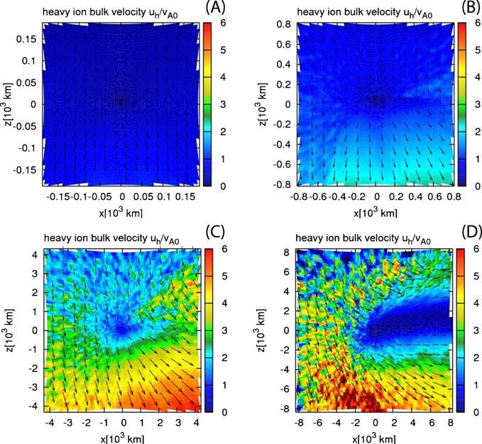
THE PLASMA ENVIRONMENT OF COMET 67P/CG                      135

the neutral gas are very strongly coupled by ion-neutral collisions, and they move
radially outward with the same expansion velocity.
    Complexities in this basic picture arise for weaker production rate comets where
the sizes of cometosheath and/or the bow shock standoff distance would be compa-
rable to or even smaller than the ion gyroradius (Bagdonat and Motschmann, 2002a;
Lipatov et al., 2002). This will be shown to be especially important at the time of
the Rosetta – 67P/CG rendezvous when the production rate is very low. At this
time, the classical ideas of bow shocks and diamagnetic cavities are meaningless.
The complex nature of the solar wind – comet interaction for weak production rate
can be further complicated by the large difference between the gyroradii of protons
(1 amu) as opposed to heavy ions (∼18 amu).
    For relatively active comets, the electron component of the plasma is derived
from multiple sources and cannot be simply described with a Maxwellian distri-
bution function. There are three possible electron sources near the comet (Gan
and Cravens, 1990): (1) the solar wind, or shocked solar wind, electrons which
travel down magnetic field lines into the cometary coma, (2) secondary electrons
produced by the impact of solar wind electrons which have sufficient energy to
ionize cometary neutrals, and (3) photoelectrons produced by photoionization of
cometary neutral gas by solar extreme ultraviolet and soft x-ray photons. Each of
these electron populations is modified through its collisional interaction with the
neutral gas and with the cometary plasma close to the comet. If the cometary gas
and plasma is dense enough then a relatively cold thermal electron population can
exist in the cometary coma.
    The application of global simulation models to the study of the cometary plasma
environment has been a valuable tool in understanding not only the general struc-
ture of the steady-state solar wind – comet interaction, but also the effects of the
dynamic solar wind. A significant, early use of global models of the cometary
environment was to study Comet 1P/Halley and data derived from the flybys of
the Giotto spacecraft. Wegmann et al. (1987) published a magnetohydrodynamic
(MHD) model which favorably compared to the HIS ion mass spectrometer on the
Giotto spacecraft and was able to study the plasma environment both inside and
outside the contact surface. Following this initial use of MHD to model the comet
environment during spacecraft flybys, the Schmidt-Wegmann model has been used
to study a series of data sets including comet 21P/Giacobini-Zinner (Huebner et al.,
1989), the Giotto encounter with comet 26P/Grigg-Skjellerup (Schmidt et al., 1993)
and the plasma tail of comet Austin 1990 V (Wegmann et al., 1996). During this
same period, an adaptive mesh model of the cometary environment was introduced
and was also used to study the Giotto encounter with comet 1P/Halley (Gombosi
et al., 1996). This model, which is used in this paper, has subsequently been used
to perform a number of simulations of the cometary environment. Many of these
studies use results from the MHD model to feed into other models of the comet
environment to study diverse topics such as the detailed ion chemistry of comets
1P/Halley (Häberli et al., 1997), Hale-Bopp (Gombosi et al., 1999), and Hyakutake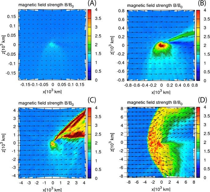
136                               K. C. HANSEN ET AL.

(Lovell et al., 2004), the x-ray emission of comets due to charge exchange of high
charge state solar wind ions (Häberli et al., 1997), and several detailed studies
of the plasma environment of comet Halley (Israelevich et al., 1997, 2000, 2003;
Tatrallyay et al., 1997, 2000). More recently, a new multi-fluid MHD model has
been introduced and used to study the Giotto flyby of comet 26P/Grigg-Skjellerup
with results being extrapolated to comet 67P/Churyumov-Gerasimenko, the Rosetta
target (Benna and Mahaffy, 2006).
    In addition to steady-state models of the cometary environment, global MHD
models have been used to study dynamics events such as ion-tail disconnections.
The first of these studies addressed the effect of interplanetary shocks on the
cometary ion tail (Wegmann, 1995). This study showed that tail rays and a tailward
moving ion cloud resembling tail disconnection events results from compression
due to an interplanetary shock. Follow on studies have considered the effect of var-
ious tangential discontinuities including a change in the solar wind flow direction
and a 90◦ rotation of the magnetic field (Rauer et al., 1995) which also show some
characteristic features of cometary ion tails. Work by Yi et al. (1996) studied how
crossing the heliospheric current sheet affects the ion tail and point to these crossing
as being the cause of most tail disconnection events. The cause of disconnection
events is still controversial and not with the scope of this paper, but global MHD
models of this type of phenomena are leading to a better understanding of how the
heliospheric environment affects comets.
    Finally, as outlined above, weak comets may not be well described by MHD mod-
els. In order to study the solar wind interactions with low production rate comets,
hybrid models have been developed. These simulations, which treat comets in the
kinetic regime, show the effect of cycloid motion of the picked up cometary ions
and the induced asymmetries (Lipatov et al., 1997, 2002; Motschmann and Kührt,
2006). A recent application of hybrid models studied the transition of the cometary
environment from a kinetic-dominated regime to a fluid-dominated regime (Bag-
donat and Motschmann, 2002b) with specific application to comet 46P/Wirtanen
(which was the intended Rosetta target before the change to 67P/CG). The study
examines cometary ion structures as they transition from the classical bow shock,
diamagnetic cavity structure of strong comets to the cycloidal tail and non-liner
Mach cones typical of weak comets. In this paper, we repeat a similar study for the
new Rosetta target, comet 67P/CG.

               2. Expected Activity and Solar Wind Parameters

Comet 67P/CG has been observed on a number previous perihelion passages, but
not intensively. Once it was identified as the Rosetta target – well after the most
recent perihelion passage – a more concerted effort was begun to monitor at least
its outgoing leg (Schulz et al., 2004; Weiler et al., 2004). We have chosen to model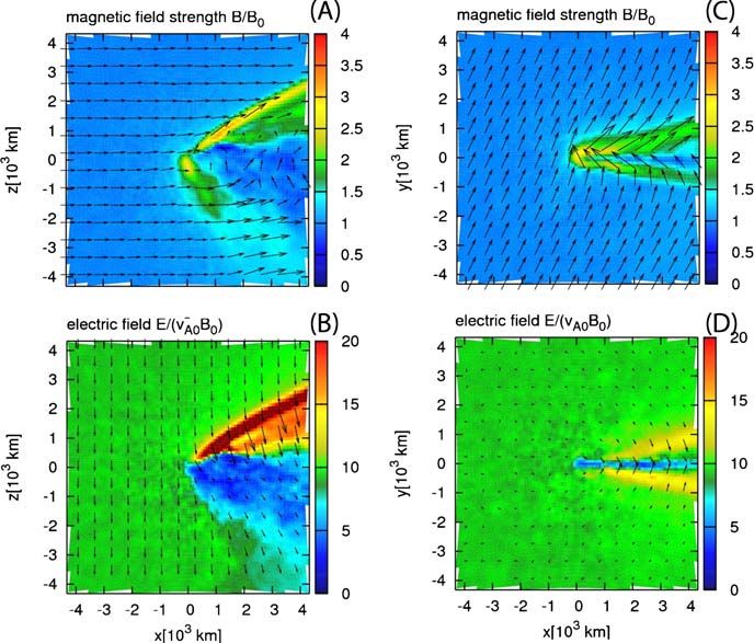
THE PLASMA ENVIRONMENT OF COMET 67P/CG                                       137

                                          TABLE I
                Solar wind conditions used for the plasma environment models.

           Location & status                                     Solar wind

 Case   Rosetta status      R(AU)      n(cm−3 )    v(km/s)    v A (km/s)    B(nT)      Angle   E(mV/m)

 a      Instruments on      3.25       0.9         400        36.8          1.6        73      1.54
 b      Lander down         2.7        1.4         400        36.9          2.0        70      1.00
 c                          2.0        2.5         400        38.7          2.8        63      0.75
 d      Perihelion          1.3        6.0         400        43.7          4.9        52      0.61

                                         TABLE II
                 Cometary parameters used for the plasma environment models.

                                   Location & status             Neutral coma

                     Case    Rosetta status       R (AU)     Q (s−1 )      λ (km)

                     a       Instruments on       3.25       1 × 1024      1.1 × 10⁷
                     b       Lander down          2.7        8 × 1025      7.3 × 10⁶
                     c                            2.0        8 × 1026      4.0 × 10⁶
                     d       Perihelion           1.3        5 × 1027      1.7 × 10⁶

the comet at four representative heliocentric radial distances that represent either
significant times of the mission or serve to span the range of plasma environments
that can be expected during the mission (see Tables I and II).
   In order to model the comet for the cases listed in Table I, we must choose
representative solar wind conditions. So that the models will be reasonably self
consistent, we have based the solar wind conditions on nominal values at 1 AU. At
that location we use u = 400 km/s, n = 10 cm−3 , Te = 1 × 10⁵ K, Ti = 5 × 10⁴
K and B = 7nT confined to the ecliptic plane, making an angle representative of
the Parker spiral at 1 AU. We then use an extrapolation to obtain the conditions
for each of the cases. Table I gives values in the upstream solar wind for density
(n), velocity (v), magnetic field magnitude (B) and Parker spiral angle, the Alfvén
speed (va ), and the electric field (E). Clearly these values are only representative
of the conditions that comet 67P/CG may encounter during the Rosetta mission,
however as average values they will give a good idea of the type and scale of the
expected interaction between the comet and the solar wind.
   The solar wind is known to be highly variable and these variations affect the
conditions experienced by comets in the heliosphere. It is possible to model the
range of different conditions using a series of steady state simulations with varied
upstream parameters. However, to accurately capture the effect of quickly varying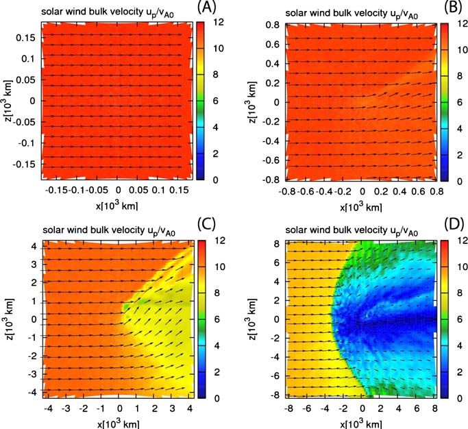
138                               K. C. HANSEN ET AL.

conditions it is necessary to simulate dynamics events such as solar wind com-
pression events or heliospheric current sheet crossings. Such studies are beyond the
scope of this paper as we wish to provide a general idea of the size and characteristic
of the cometary environment of comet 67P/CG throughout the Rosetta mission in
an average sense. However the effects of interplanetary shocks (Wegmann, 1995),
magnetic field rotations (Rauer et al., 1995) and heliospheric current sheet cross-
ings (Yi et al., 1996) have previously been studied using MHD models and the
results of those studies can be applied to comet 67P/CG when the comet is near
perihelion. No studies of dynamic events have been done for weak comets using
hybrid simulations.
    The cometary plasma environment, as outlined in the introduction, is driven
by the ionization of the neutral coma. Therefore, any plasma model must either
include a prescribed or a self-consistent model of the neutral distribution and its
interaction with the plasma. Table II indicates the values of the cometary neutral
production rate which are applied in the models presented in this paper. The neutral
distribution is taken to be a simple spherically symmetric source which expands at
constant velocity.
             Q           r
    nn =            exp  −                                                          (1)
          4πu n r 2        λ
where Q is the gas production rate, u n = 1 km/s is the radial neutral velocity,
r is the distance from the nucleus and λ is the ionization scale length. Both the
gas production rate, Q, and the ionization scale length, λ, depend on heliocentric
distance. Table II indicates the values for these parameters that we have adopted
in this paper. Given this neutral distribution and the ionization scale length (or
equivalently the ionization rate) both the hybrid and MHD models described below
can produce models of the comet’s plasma environment.

                         3. Plasma Environment Models

In this paper we concentrate on only the plasma component of the cometary envi-
ronment and apply our models specifically to comet 67P/CG, the Rosetta target. We
have applied two different models to the solar wind – comet interaction: a Hybrid
and an MHD model of the plasma.
    As outlined in the previous section, 67P/CG is a fairly typical Jupiter-Family
comet. The comet’s low gas production rate near the beginning of the Rosetta mis-
sion results in the cometary boundaries (bow shock, Mach cone, contact surface,
etc.) that move closer to the comet. The result is that the gyroradius of ions, either
newly picked-up or of solar wind origin, is quite large compared to the extent of
67P/CG’s plasma structures. While the comet is in this regime, a model which
includes finite-gyroradius effects is required to accurately describe the plasma. For
this reason, we have included a semi-kinetic hybrid particle model of the plasma.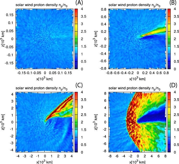
THE PLASMA ENVIRONMENT OF COMET 67P/CG                        139

However, when 67P/CG is closer to perihelion and the gas production rate is signif-
icantly larger, the finite gyroradius effects are smaller and a fluid description of the
plasma becomes valid. For this reason we also consider a magnetohydrodynamic
(MHD) model of the plasma. Each of these two models has different strengths and
weakness which we describe below.
    In the two models, an empirical neutral distribution described above is used to
compute the effects of mass loading and collisions. Because the models do not
directly model the many different cometary ions, nor the neutral distribution, there
is no reason to compute the ionization, charge exchange and collision terms in
minute detail. Therefore, mass addition in both models is handled via an effective
ionization rate (described above). The rate is chosen to include contributions from
both photoionization and charge exchange. Similarly, in each model the effects of
ion-neutral collisions as well as the momentum exchange effects of charge exchange
are handled through a friction term where the effective friction coefficient is chosen
to include, in an average sense, all relevant collisional processes. In detail, these
processes are handled in slightly different ways by the two models due mostly to
differing numerical techniques. In the following sections we give references for
each of the two models.
    For the perihelion case, we additionally include a two–stream transport model
of the electron population. This model provides information about the suprathermal
electrons along magnetic field lines threaded through the cometary coma.

3.1. T HE H YBRID MODEL

Hybrid codes have been successfully applied to space plasmas over the past 20 years
(Brecht, 1997; Winske, 1985; Winske et al., 2003, and references therein). In this
paper we apply the hybrid model of Bagdonat et al. (2002a,b) with only minor
modifications. We describe below only the very basic features of the model and
refer the reader to the above references for a detailed description of the methods
used.
   A hybrid model describes the plasma environment in a semi-kinetic manner. In
the model, electrons are assumed to be a massless charge-neutralizing fluid and
are modeled using typical fluid methods (conservation equations). The ions, which
have much larger gyroradii, are treated as particles and the code solves individual
equations of motion. This method resolves physical structures down to a time scale
below the inverse lower hybrid frequency.
   The hybrid model that we employ considers two ion species: the solar wind
protons and the ions of cometary origin. These cometary ions are significantly
heavier than the solar wind protons. In order to correctly model the ions, the dynamic
equations include collisions with neutral gas in addition to the Lorentz force. This
driver may become significant in dense atmospheres such as near the cometary
nucleus.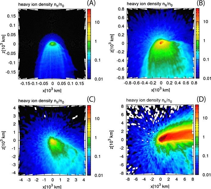
140                                    K. C. HANSEN ET AL.

    The electrons in the model interact with the ions mainly by virtue of their
pressure. We consider only a single electron fluid, but take into account the fact
that the temperature and the ratio of gas to magnetic pressure, expressed by the
plasma beta, are significantly different in the case of the electrons in the solar
wind compared to those of ionospheric origin. The consideration of these different
electron temperatures is described by Bagdonat et al. (2004).
    Because the solar wind flow is supersonic, information from the solar wind –
comet interaction does not travel upstream and therefore simple boundary condi-
tions can be chosen. Upstream we use a constant inflow boundary where newly
inserted particles have a thermal distribution and all field quantities are kept con-
stant. Downstream we apply an outflow boundary where all particles which cross
the boundary (leave the box) are deleted. All field quantities are linearly extrapo-
lated from the upstream side. All other boundaries are either periodic, in the case
of a rectangular simulation box, or also inflow-/outflow-boundaries in the case of
non-orthogonal grids.
    We present results of both 2D and 3D hybrid models of 67P/CG. We describe
the 3D grid structure here and point out that the 2D structure is similar, but quite
a bit simpler to understand and to implement. The hybrid model of Bagdonat and
Motschmann (2002b) operates on a three dimensional (3D) grid which is static but
curvilinear. The grid is hexahedral (each cell has six faces) and ordered, so that
each grid point can be described by a triple index. For the cometary case the grid,
as shown in Figure 1, is advantageous. The spatial resolution is increased in those
regions where significant small-scale processes take place.
    The use of the curvilinear grid implies serious technical challenges. For example,
if there were a constant ion density across the entire grid the large cells would have

Figure 1. Structure of curvilinear simulation grid used in the hybrid model of the interaction of the
solar wind with a comet. The point-like nucleus is at the origin.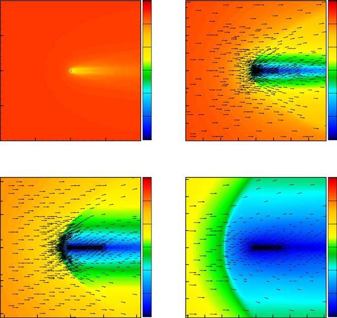
THE PLASMA ENVIRONMENT OF COMET 67P/CG                        141

significantly more particles in them then the small cells, especially in the 3D version
of the code. Of course this leads to a huge loss of computing efficiency. To overcome
this, we use particle coalescence to control the number of particles in a cell. The
code has been tested intensively and successfully applied not only to weak comets
(Bagdonat and Motschmann, 2002a,b; Bagdonat et al., 2004) but also to other weak
obstacles such as asteroids (Simon et al., 2006a), Mars (Bößwetter et al., 2004) and
Saturn’s moon Titan (Simon et al., 2006b).
    For the simulations in Section 4.1 each of the figures shows the entire simulation
domain. This domain is chosen in such a way that important potential plasma
signatures near the nucleus are covered, especially the bow shock, cometopause
and diamagnetic cavity. Distant tail structures are not captured by the currently used
domains and are beyond the scope of this study. Simulations in 2D are performed
on a 200 × 200 grid while in 3D the grid is 90 × 90 × 90. In each case, the smallest
cell at the nucleus is about one third the size of the largest at the box boundaries.
The runs become quasi-stationary after about 5000–7000 time steps and all results
are presented after 9000 time steps.

3.2. T HE MHD MODEL: BATSRUS

In order to model 67P/CG when its plasma can be described accurately as a fluid,
we are using the global, 3D magnetohydrodynamic (MHD) code BATSRUS (Block
Adaptive Tree Solarwind Roe-Type Upwind Scheme). The code solves the gov-
erning equations of ideal magnetohydrodynamics. In the MHD limit, the plasma
is treated as a single species plasma. Effects related to finite gyroradius, resistivity
and other kinetic effects are neglected. However, we are able to describe some non-
MHD effects by describing these deviations from ideal MHD (sources and sinks of
mass, momentum and energy, or resistive and diffusive processes) through appro-
priate source terms. Here we present a few details about the aspects of BATSRUS
that are relevant to the solar wind – comet interaction and refer the reader to an
extensive literature related to the numerical algorithms used in the code. A review
of many of the fundamental aspects of the model algorithms is found in Powell
et al. (1999). Details of how the cometary environment is modeled with BATSRUS
can be found in Gombosi et al. (1996) and Gombosi et al. (1999) in addition to
the many papers which apply BATSRUS results to the study of several different
comets (Haberli et al., 1997a,b; Israelevich et al., 1999, 2000, 2003; Lovell:2004;
Tatrallyay et al., 1997, 2000).
    One of the most important features of BATSRUS is the ability to easily adapt
the grid to resolve specific regions of space. BATSRUS utilizes the approach of
adaptive blocks (Powell et al., 1999; Stout et al., 1997). Adaptive blocks parti-
tion space into regions, each of which is a regular Cartesian grid of cells, called
a block. If the region needs to be refined, then the block is replaced by 8 child
sub-blocks, each of which contains the same number of cells as the parent block.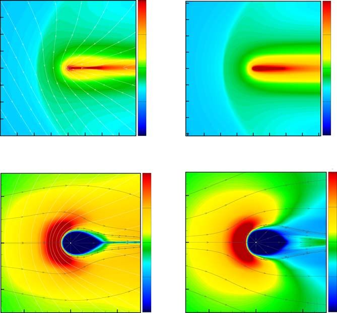
142                                                       K. C. HANSEN ET AL.

                                                         TABLE III
                                                    MHD model grid cell sizes.

                         Location & status                            Domain (km)

     Case             Rosetta status       R (AU)        Min x      Max x            Boundary (+x)        Refinement levels

     a                Instruments on       3.25          0.06        250               2,000                12
     b                Lander down          2.7           0.06        250               2,000                12
     c                                     2.0           0.06        7,500             60,000               17
     d                Perihelion           1.3           0.5         2.5 × 10⁵         4 × 10⁶              19

             -4

                                                                                 -40

             -2
                                                                                 -20
 Z [10 km]

                                                                        Z [km]

             0                                                                    0
 3

                                                                                 20
             2

                                                                                 40

             4
                  4          2         0            -2          -4                     40        20     0        -20     -40
                                       3
                                   X [10 km]                                                          X [km]

Figure 2. Example of the adaptive grid used in the MHD (BATSRUS) model for simulation of case
b (2.0 AU). The left figure shows the grid in the region of the bow shock, while on the right we show
the grid in the region of the diamagnetic cavity and the nucleus.

The use of cells of varying sizes allows us to resolve features of vastly different
length scales. In the simulations presented in this paper, we are able to resolve
the body, the diamagnetic cavity and the solar wind – neutral cloud interaction
even though these occur at vastly different length scales (see Figure 2). Table III
indicates smallest and largest cell sizes as well as the size of the simulation do-
main for the MHD simulations in this paper. Note that the adaptive mesh allows us
to use an extremely large simulation box and therefore self-consistently model
the mass loading and subsequent slowing of the plasma upstream of the bow
shock.
    In the model all processes associated with mass loading (ionization, charge ex-
change, recombination, etc.) are handled through appropriate sources terms. These
are implemented in the same manner as the source terms used in our previous study
of the comet Hale-Bopp (Gombosi et al., 1999). Differences from that paper only
THE PLASMA ENVIRONMENT OF COMET 67P/CG 143
require adjusting the gas production rate to that of comet 67P/CG and adjusting the
photoionization scale length for heliocentric distance.
For the MHD simulations presented in this paper, the cometary nucleus is treated
as a 2.5 km radius hard sphere. Having an actual body in the simulation is not
important near perihelion where the scale of the solar wind – comet interaction is
very large, but the small size of the interaction at 3.25 AU requires a body. In the
model, where the radial velocity (vr ) at the surface is into the body, the density,
pressure and vr are forced to have a zero gradient and therefore mimic an absorbing
sphere. For other cells where the radial velocity just outside the body is outward, vr
is set to zero at the body and the pressure and density are fixed to small values. This
assures that the body itself is not a large source of plasma. The velocity parallel
to the body and all three components of the magnetic field are forced to have zero
gradients, thus in effect allowing their values to float. We do not solve equations
inside the body.
3.3. T HE E LECTRON M ODEL
As describe above, the electron component of the plasma is not a simple Maxwellian
due to the several electron sources including the shocked and unshocked solar
wind, secondary electrons produced by the impact of solar wind electrons and
photoelectrons. In each case, collisions with the neutral gas of the cometary coma
modifies the electrons as they travel along magnetic field lines.
In this paper we present a model of the 67P/CG electron population using meth-
ods described by Gan and Cravens (1990). Gan constructed a model of the spatial
and energy distributions of electrons in the vicinity of comet Halley. The method in-
volves the calculation of suprathermal electron fluxes using a two-stream transport
technique which included electron impact cross sections for rotational, vibrational,
and electronic excitation of water molecules. Their model also calculated electron
temperatures for the thermal electron population and found that cold, “ionospheric”
electrons should indeed be present for cometocentric distances less than a few thou-
sand km.
The Rosetta target comet, 67P/Churyumov-Gerasimenko, even near perihelion,
is a considerably weaker comet than Halley was in 1986. Nonetheless, we have
undertaken electron modeling for this comet near perihelion using the methods
described in Gan and Cravens (1990). In our model, the electron transport is
constrained by the magnetic field topology which we have extracted from the
perihelion results of the MHD model discussed above. For the results presented
here, the field line shape is approximately parabolic over the region of the coma
where the calculation occurs. In principle, the model can be used for any field
line which threads the coma, however below we present results from a repre-
sentative field line which crosses the Sun-comet line at 50 km upstream of the
nucleus.144 K. C. HANSEN ET AL.
4. Results
4.1. H YBRID MODEL RESULTS
The hybrid model regards solar wind protons and cometary ions as separate species.
As the cometary ions are much heavier than the solar wind protons, hereafter we
use the phrases “heavy ions” and “cometary ions” synonymously when referring
to ions whose source is the comet. In the following discussion the subscript p
refers to solar wind protons while cometary ions are indicated by the subscript
h. In Figures 3 to 10 we present cometary ion density n h , cometary ion velocity
u h , solar wind proton density n p , solar wind proton velocity v p , magnetic field
B and electric field E as our standard parameters. We first discuss 2-dimensional
(2D) simulation results followed by a brief discussion of a 3-dimensional (3D)
case. The 2D simulation plane contains the undisturbed solar wind flow velocity
Figure 3. 2D hybrid model results of the cometary ion density n h at heliocentric distances of 3.25 AU
(A, upper left), 2.7 AU (B, upper right), 2.0 AU (C, lower left), and 1.3 AU (D, lower right). This
density is normalized to the undisturbed solar wind density n 0 .THE PLASMA ENVIRONMENT OF COMET 67P/CG 145 (x axis) as well as the undisturbed interplanetary electric field (negative z axis). The undisturbed interplanetary magnetic field lies in the x-y plane (perpendicular to the simulation plane). In principle 2D and 3D simulations qualitatively reproduce the same cometary evolution with the same characteristic plasma structures, however the location of the structures shifts. In 3D the tendency is that the interaction region becomes smaller and the spatial scales are compressed. The effect is much less than one order of magnitude, it is on the order of a factor 2. The advantages of the 2D simulations are better particle statistics and therefore less noisy simulation results. 4.1.1. 2D Simulation Results The 2D simulation results are presented in Figures 3 to 8. Let us start with the evolution of the cometary ion density n h shown in Figure 3 and the corresponding cometary ion velocity vh shown in Figure 4. Far away from the sun at 3.25 AU the cometary activity is extremely weak and the cometary plasma is extremely faint. Figure 4. 2D hybrid model results of the cometary ion velocity vh at heliocentric distances of 3.25 AU (A, upper left), 2.7 AU (B, upper right), 2.0 AU (C, lower left), and 1.3 AU (D, lower right). This velocity is normalized to the Alfvén velocity in the undisturbed solar wind.
146                                K. C. HANSEN ET AL.

The cometary ions behave mainly like test particles. The loading of the solar wind is
thus small so that there is no major modification of the solar wind parameters. The
pickup process of freshly ionized cometary particles directs them perpendicular to
the solar wind flow as is clearly seen in Figure 3A. This perpendicular cometary
ion tail may be counter intuitive to those familiar with the ion tails of comets
which exhibit fluid-like behavior, however, its generation mechanism is simple. All
cometary ions feel mainly the Lorentz force
   Fh = q (E + vh × B) .                                                              (2)
For the present discussion, any friction forces may be neglected. As the velocity of
the newborn cometary ions near the nucleus is very small (vh ≈ 0) they feel mainly
the electric force q E where E is the interplanetary convective electric field
   E = −v p × B.                                                                      (3)
Thus the force to the cometary ions is
   Fh = −qv p × B                                                                     (4)
which is perpendicular to the solar wind flow velocity v p . Therefore the initial stage
of the cometary ion tail is just perpendicular to the solar wind flow. Later on, when
the cometary ions are accelerated to a finite velocity (vh > 0) they also feel a signif-
icant force qvh × B which causes cycloidal trajectories for each individual particle.
Figure 3A shows the early beginning of these cycloids. A quite similar behavior
was observed at the artificial comet of the AMPTE/UKS experiment (Haerendel
et al., 1986).
    At 2.7 AU the activity of the comet has increased. Figure 3B shows that the
maximum cometary ion density has grown by a factor of 10 compared to 3.25 AU.
Near the nucleus the cometary ion density, n h , is higher than the solar wind proton
density, n p , by a factor of 5 as seen by comparison of Figures 3B and 5B. Thus,
the feedback of the cometary ions to the solar wind is no longer negligible. The
ion tail still has a pronounced perpendicular component but it rotates slightly into
the solar wind flow. The ion tail follows the rotation of the electric field which
will be discussed below. This rotation of the cometary ion tail continues during
the further approach of the comet to the sun. At 2.0 AU, Figure 3C shows an ion
tail where parallel and perpendicular flow components are already of comparable
strength. At 1.3 AU the ion tail is mainly anti-sunward. Actually, Figure 3D shows
some deviation in +z direction. The ion tail rotation is accompanied by a strong
extension of the coma and the whole plasma interaction region. Comparison of
Figure 3A and 3D demonstrates a difference in spatial extent of about two orders
of magnitude.
    Let us now discuss the solar wind density, n p , and the corresponding velocity, v p ,
in more detail. Figures 5A and 6A demonstrate once more the absence of significant
feedback of the faint comet at 3.25 AU to the solar wind parameters. At 2.7 AU a
cone like downstream structure is highlighted in Figures 5B and 6B. This structure
THE PLASMA ENVIRONMENT OF COMET 67P/CG 147 Figure 5. 2D hybrid model results of the solar wind proton density n p at heliocentric distances of 3.25 AU (A, upper left), 2.7 AU (B, upper right), 2.0 AU (C, lower left), and 1.3 AU (D, lower right). This density is normalized to the undisturbed solar wind density n 0 . is just the indication of a Mach cone which is caused by the cometary obstacle in the superfast solar wind flow. The actual obstacle is not the comet itself, but is the region of high cometary ion density, n h , very near to the nucleus. An ideal, symmetric Mach cone would be excited by a point like obstacle. However, the cometary coma, combined with the pick-up process, present an obstacle which is rather asymmetric causing an asymmetric shape of the Mach cone. Further approach of the comet to the sun evolves the Mach cone as depicted in Figures 5C and 6C. A bow shock is not yet seen at the heliocentric distance of 2.0 AU, however the bow shock has clearly arisen at 1.3 AU as demonstrated in Figures 5D and 6D. The subsolar bow shock position is at about 3000 km. For the perihelion case, the hybrid model predicts a gyroradius of picked-up oxygen ions of ≈13, 000 km and for solar wind protons of ≈80 km just in front of the bow shock. We note, however that small simulation box does not allow for the upstream mass loading to slow the plasma and that if this effect were included the gyroradius of both species would be further reduced.
148                                     K. C. HANSEN ET AL.

Figure 6. 2D hybrid model results of the solar wind proton velocity v p at heliocentric distances of
3.25 AU (A, upper left), 2.7 AU (B, upper right), 2.0 AU (C, lower left), and 1.3 AU (D, lower right).
This velocity is normalized to the Alfvén velocity in the undisturbed solar wind.

    Figures 7 and 8 show the evolution of the magnetic field, B, and the electric field,
E. Starting at 3.25 AU the B and E fields confirm our expectation that the faint
coma has only very weak feedback on the solar wind parameters. At 2.7 AU the
magnetic field perturbation (Figure 7B) lies along the perpendicular cometary ion
tail and is a good indicator of the Mach cone. Typically, the field strength fluctuates
by 50 per cent with respect to the background. Very near to the nucleus the magnetic
pile up is about 300 percent. We note that in this 2D simulation the undisturbed
solar wind magnetic main component points into the page (B y > 0). The smaller
x component points along the x axis (Bx = 0). Both components are chosen to
correspond to Parker’s solar wind model. Thus the magnetic field lines may slide
over the nucleus and no conflict with the 2D model is caused. At 2.0 AU the magnetic
field still has a cone-like shape whereas at 1.3 AU the bow shock is fully developed.
The jump of the magnetic field strength at the bow shock is about 3.5 near the
subsolar region. The evolution of the electric field may be followed in Figure 8.
THE PLASMA ENVIRONMENT OF COMET 67P/CG 149 Figure 7. 2D hybrid model results of the magnetic field B at heliocentric distances of 3.25 AU (A, upper left), 2.7 AU (B, upper right), 2.0 AU (C, lower left), and 1.3 AU (D, lower right). This field is normalized to the undisturbed magnetic field in the solar wind. The main component of B points into the plane and it is not to be seen in the arrow plot. The color representation shows the full value of B. The normalized, undisturbed electric field strength is about 10. This number varies slightly with the heliocentric distance as our electric field normalization is coupled to the Mach number. The exact undisturbed normalized electric field values are 11.2 at 3.25 AU, 11.0 at 2.7 AU, 10.5 at 2.0 AU and 9.3 at 1.3 AU. The direction of the undisturbed electric field is always the negative z axis. The electric field maps the plasma structures in a way analogous to the magnetic field. However, additional insight into cometary plasma dynamics comes from the study of the direction of the electric field. To simplify notation let us introduce the directions north (positive z direction), south (negative z direction), east (positive x direction, anti-sunward) and west (negative x direction, sunward). The undisturbed solar wind electric field points south (see Equation (3)) while our choice of a magnetic field points into the plane (positive y direction). For an alternative choice of a magnetic field pointing out of the plane the electric field would point north and for all subsequent structures
150                                   K. C. HANSEN ET AL.

Figure 8. 2D hybrid model results of the electric field E at heliocentric distances of 3.25 AU (A,
upper left), 2.7 AU (B, upper right), 2.0 AU (C, lower left), and 1.3 AU (D, lower right).

north and south would exchange. When the solar wind approaches the cometary
obstacle it is deflected around the obstacle as shown in Figure 6. The predominant
solar wind deflection is northward and the reaction of the electric field is an eastward
rotation because of Equation (3) which is to be seen in Figure 8B and 8C.

4.1.2. Boundaries in the Cometary Plasma Environment
Two major plasma boundaries may be identified in the plasma environment of the
comet by the hybrid simulations. One boundary is the bow shock. It forms within
2.0 AU and it is fully developed at 1.3 AU. Beyond 2.0 AU the precursor of the bow
shock is the Mach cone which is mapped in the solar wind proton data (see Figures 4
and 6) and in the fields (see Figures 7 and 8). With increasing cometary activity the
Mach cone develops more fully and eventually forms the bow shock. The second
boundary is a jump in the cometary ion density. In the cometary community several
descriptions are in use for this jump, e.g. cometopause, ion composition boundary
and heavy ion density jump. This jump evolves as a function of the heliocentric
THE PLASMA ENVIRONMENT OF COMET 67P/CG                        151

distance and as it develops a strong asymmetry the different terms vary in their
appropriateness. In contrast to the bow shock this heavy ion density jump exists
not only near perihelion but also in larger heliocentric distance. Let us follow the
evolution of this jump (see Figure 3). The density jump may be identified already at
3.25 AU when the cometary ion density is very faint. The ion tail points southward.
The northern and the western edges of the tail are very steep and form the early
stage of the boundary. The description as a cometopause for this jump is appropriate,
however the term ion composition boundary is not as the solar wind completely
penetrates the ion tail. Increasing cometary activity at 2.7 AU and 2.0 AU prevents
the ion tail penetration more and more and deflects the solar wind protons. This
process has the tendency to separate the solar wind protons and the cometary ions.
A nearly complete separation is reached at 1.3 AU. Proton density and cometary ion
density behave complementary as can be seen in Figures 3D and 4D. At perihelion
the descriptions ion composition boundary and cometopause are both justified.

4.1.3. 3D Simulation Results
3D hybrid simulations should in principle lead to a more accurate picture of the solar
wind – comet interaction than comparable 2D simulations. However, the increased
computational effort required for 3D simulations is enormous and therefore cell
resolutions and particle statistics must be reduced. For this reason, the 2D and 3D
simulations should be thought of as complimentary: 2D provides better resolved
results and insight into the basic interaction features while 3D locates these features
more accurately and provides insight into differences between the ecliptic plane
(which contains the upstream solar wind) and the polar plane. Additionally, the 3D
simulations provide an additional degree of freedom for the plasma motion and
allow the magnetic field lines to drape around the cometary coma, a feature that
cannot be present in the 2D models.
    Figures 9 and 10 represent 3D hybrid model results for a heliocentric distance
of 2 AU. Overall, the 3D results in the x-z plane capture the same qualitative picture
of the solar wind – comet interaction as do the 2D results. Quantitatively, differ-
ences include the fact that the interaction region is smaller and also include small
differences in the magnitudes of various plasma quantities. For the presentation we
cut the 3D data in the x-z plane (which we call the polar plane) and in the x-y plane
(which we call ecliptic plane). The polar plane corresponds to the 2D simulation
plane. Our standard parameters are shown in Figures 9 and 10. In the 3D results the
obstacle generally appears to be weaker compared to the 2D case. One reason for
this is the presence of a third direction in which the solar wind can flow around the
obstacle. This additional degree of freedom naturally tends to weaken the feedback
to the solar wind. Another reason is the much stronger magnetic field line curvature
force in the 3D situation compared to the 2D situation. This force accelerates the
cometary ions in the anti-sunward direction, forming the main ion tail. It leads to
a more efficient transport of heavy ions away from the nucleus which makes the
obstacle to appear effectively weaker than in the 2D case. The 3D results probably
152 K. C. HANSEN ET AL. Figure 9. 3D hybrid model simulation results at heliocentric distance of 2 AU. Cometary ion density n h (A, E), solar wind proton density n p (B, F), cometary ion velocity vh (C, G), solar wind proton velocity v p (D, H). Left panel (A – D): polar plane. Right panel (E – H): ecliptic plane.
THE PLASMA ENVIRONMENT OF COMET 67P/CG                                 153

Figure 10. 3D hybrid model simulation results at heliocentric distance of 2 AU. Magnetic field B (A,
C) and electric field E (B, D). Left panel (A – B): polar plane. Right panel (C – D): ecliptic plane.

provide a more quantitatively valid picture, but the 2D results exhibit more detail
due to the higher particle statistics. For an understanding of ROSETTA data both
types of simulation results should be considered.

4.2. MHD M ODEL RESULTS

In this section we describe results from our MHD model of the 67P/CG at the
same radial distances as described for our Hybrid model. As outlined above, the
comet – solar wind interaction is not well described by MHD when the pick-up ion
gyroradius is much larger than the scale lengths of the cometary coma. Therefore,
realistically, the MHD results are only valid for the 1.3 and 2.0 AU cases (c,d).
However, we have included the MHD model runs for the 2.7 and 3.25 AU cases for
completeness. Although in these cases the non-MHD effects associated with the
gyro-motion of the particles is very significant, we find that the MHD results do
still provide pieces of information that may be beneficial to the reader if taken in
the proper context.
154                                      K. C. HANSEN ET AL.

Figure 11. MHD model results of the Cometary mass density ρ at heliocentric distances of 3.25 AU
(A, upper left), 2.7 AU (B, upper right), 2.0 AU (C, lower left), and 1.3 AU (D, lower right). The color
contours represent the plasma mass density normalized to the upstream value, ρ0 , in the solar wind
(ρ/ρ0 ).

   Figures 11 – 15 represent the MHD model of comet 67P/CG. In each case
the figures are normalized to the upstream solar wind conditions given in Table I.
Figure 11 shows the cometary mass density for the model. We note that because the
model is single species MHD it is not possible to differentiate the solar wind protons
from the cometary ions as is possible in our Hybrid model and for this reason we
show only the mass density. The figure clearly depicts several main features of the
comet – solar wind interaction that are possible to model with MHD. At each of
the heliocentric distances, note that the cometary ions are picked-up well upstream
of the bow shock. As indicated in Table III, our adaptive mesh MHD model is
capable of modeling a very large region of space. This allows us to easily resolve
the gradual slowing of the plasma upstream of the bow shock due to the extended
THE PLASMA ENVIRONMENT OF COMET 67P/CG                                                                   155

                                                     (A)                                                                                (B)
         -0.2                                          12           -0.8                                                                  12

                                                                    -0.6
                                                       10                                                                                 10
         -0.1                                                       -0.4

                                                       8                                                                                  8
                                                                    -0.2
 Z [10 km]

                                                            Z [10 km]
              0                                        6                 0                                                                6
 3

                                                            3
                                                                        0.2
                                                       4                                                                                  4
             0.1                                                        0.4

                                                       2                                                                                  2
                                                                        0.6

             0.2                                       0                0.8                                                               0
                0.2    0.1      0        -0.1   -0.2                       0.8    0.6   0.4   0.2      0    -0.2     -0.4   -0.6   -0.8
                                 3                                                                      3
                             X [10 km]                                                              X [10 km]

                                                     (C)                                                                                (D)
              -4
                                                       12                -8                                                               12

                                                                         -6
                                                       10                                                                                 10

              -2                                                         -4

                                                       8                                                                                  8
                                                                         -2
 Z [10 km]

                                                            Z [10 km]

              0                                        6                 0                                                                6
 3

                                                            3

                                                                         2
                                                       4                                                                                  4
              2                                                          4

                                                       2                                                                                  2
                                                                         6

              4                                                          8                                                                0
                   4    2       0        -2     -4                            8    6     4     2       0        -2   -4     -6     -8
                                 3                                                                      3
                             X [10 km]                                                              X [10 km]

Figure 12. MHD model results of the solar wind plasma velocity v at heliocentric distances of 3.25 AU
(A, upper left), 2.7 AU (B, upper right), 2.0 AU (C, lower left), and 1.3 AU (D, lower right). The
color contours represent the magnitude of the velocity normalized to the Alfvén velocity, v A0 , in the
undisturbed solar wind (v/v A0 ). Black arrows indicate the direction and magnitude of the flow in the
depicted plane.

cometary ion pickup. The slowing can clearly be seen upstream of the shock in
both the ramping up of mass density (Figure 11) and the slowing of the plasma
velocity (Figure 12). This is a very important feature of the cometary – solar wind
interaction. Table IV shows how the pickup well upstream of the bow shock slows
and modifies the plasma for the 1.3 AU case. The plasma density just upstream of
the bow shock is 2.4 times greater than in the unperturbed solar wind and at the
same time the plasma has slowed dramatically (almost a factor of 2). The result is
that the sonic (M S ), Alfvénic (M A ) and fast magnetosonic (M F ) Mach numbers are
all greatly reduced from the upstream values. The shock is therefore very weak,
with a compression ratio of only 1.6. Additionally, we note that the magnetic field
156 K. C. HANSEN ET AL.
Figure 13. MHD model results of the magnetic field B at heliocentric distances of 3.25 AU (a, upper
left), 2.7 AU (b, upper right), 2.0 AU (c, lower left), and 1.3 AU (d, lower right). The color contours
represent the magnitude of B normalized to the upstream value, B0 , in the solar wind (B/B0 ).
is increased by about 50% over the upstream value, implying that the gyroradius
of ions is smaller than in the unperturbed solar wind.
The gradual slowing of the plasma upstream of the comet serves also to push
the solar wind – comet interaction toward the fluid regime. The plasma is slowed
and the magnetic field is compressed yielding a smaller gyroradius of both the
solar wind protons and of the pickup ions. In the perihelion case, for example, the
gyroradius of the solar wind protons and pick-up ions far upstream of the shock are
≈13, 500 km and ≈90 km respectively while just in front of the bow shock they are
reduced to ≈5, 000 km and ≈50 km. This would imply that the MHD simulation at
even 2.0 AU may be a relatively good model of the comet – solar wind interaction.
Figures 11 – 13 clearly show the cometary bow shock which forms at a crit-
ical point where the plasma has slowed sufficiently. Table V gives locations forTHE PLASMA ENVIRONMENT OF COMET 67P/CG 157
Figure 14. MHD model results of the cometary mass density ρ in the near nucleus region when 67P
is at heliocentric distances of 3.25 AU (A, upper left), 2.7 AU (B, upper right), 2.0 AU (C, lower left),
and 1.3 AU (D, lower right). The color contours represent the plasma mass density normalized to the
upstream value, ρ0 , in the solar wind (ρ/ρ0 ).
the shock standoff distance in both a sunward (+x) and in a perpendicular (−y)
directions.
At this point we highlight the fact that the 1.3, 2.0 and 2.7 AU cases all look
relatively similar and differ mainly by the scale over which the interaction occurs.
This is especially evident in Figure 13 which shows the compression of the magnetic
field behind the shock. In each of the cases, behind the bow shock we observe a
compression of the mass density and a corresponding drop in the plasma velocity.
The cometary pick-up ions form a tail in the antisunward direction. In each of the
cases, the magnetic field can be seen to “pile up” behind the bow shock and in front
of the diamagnetic cavity (which we discuss below).
The 3.25 AU case shows a quite different phenomenology. In this case the
upstream slowing of the plasma is small and is not sufficient to cause a bow shock158 K. C. HANSEN ET AL.
(A) -20
(B)
-20 10
5
-10 -10 7.5
3.75
Z [km]
Z [km]
0 2.5 0 5
10 1.25 10 2.5
20 0 0
20 10 0 -10 -20 20 10 0 -10 -20
X [km] X [km]
(C) (D)
10 10
-40
-200
7.5 7
-20
Z [km]
Z [km]
0 5 0 5
20
2.5 2
200
40
0 0
40 20 0 -20 -40 200 0 -200
X [km] X [km]
Figure 15. MHD model results of the magnetic field B in the near nucleus region when 67P is at
heliocentric distances of 3.25 AU (A, upper left), 2.7 AU (B, upper right), 2.0 AU (C, lower left), and
1.3 AU (D, lower right). The color contours represent the magnitude of B normalized to the upstream
value, B0 , in the solar wind (B/B0 ). Gray lines represent the plasma streamlines.
to form upstream of the comet. The model predicts a shock will form at the body
and extend tailward. No ion tail forms, and in fact the plasma density behind the
body (tailward) is lower than the upstream solar wind density because the body acts
to create an evacuated region.
Figures 14 and 15 show the innermost part of the comet – solar wind interaction.
In each of the figures we have zoomed in by a factor of 10–20 times from Figures 11
and 13. The simulations each include a body which is 2.5 km in diameter. Figure 14
shows the plasma mass density near the comet for each of the four heliocentric dis-
tances. For the three cases closest to the Sun (b, c, d) the plasma is mostly comprised
of cometary ions although the exact fraction cannot be determined in MHD. ForTHE PLASMA ENVIRONMENT OF COMET 67P/CG 159
TABLE IV
MHD model parameters near the bow shock at 1.3 AU.
Parameter Value in solar wind Upstream of shock Downstream of shock Jump ratio
n/n 0 1.0 2.4 3.9 1.6
v/v A 0 9.2 5.0 3.0 0.6
B/B0 1.0 1.5 2.3 1.6
MS 9.4 1.5 0.8 0.5
MA 9.3 5.2 2.6 0.5
MF 6.6 1.4 0.7 0.5
TABLE V
MHD model bow shock and diamagnetic cavity locations.
Bow shock Diamagnetic cavity
Case R (AU) +x axis −y axis +x axis −y axis
a 3.25 3,600 9,500 38 49
b 2.7 590 1,500 6.5 7.3
c 2.0 58 150 – –
d 1.3 – – – –
cases c and d (1.3 and 2.0 AU) we see that the flow of neutrals radially outward from
the nucleus, coupled with the photoionization and the ion-neutral collision results
in outward plasma flow (Figure 15 shows the plasma streamlines) which resists the
incident, compressed solar wind/pickup ion flow. This outward flow is supersonic
and therefore results in three different discontinuities. The outermost of these is
the surface which separates the upstream flow from the cometary radial outward
flow. In Figure 15 a stagnation point is evident sunward of the comet which is the
upstream limit of this surface. Because upstream, magnetized plasma is excluded
from a region near the comet, a diamagnetic cavity forms. Inside this cavity, which
has a sharp but distinct boundary, the magnetic field is zero to round-off error of the
simulation. Inside the diamagnetic cavity the supersonic plasma must pass through
a shock before it can be deflected tailward. In the simulation, this inner shock co-
incides with the diamagnetic cavity boundary to the resolution of the simulation.
Table V gives the location of the diamagnetic cavity boundary both in the sunward
(+x) and perpendicular (−y) directions for the 1.3 and 2.0 AU cases.
If we now address Figures 14 and 15 for the 2.7 and 3.25 AU cases (a,b) we see
that no diamagnetic cavity forms. The figures indicate that because of the weakness
of the upstream mass loading and the resulting size of the comet, the diamagnetic
cavity would lie inside the body and therefore does not exist.160 K. C. HANSEN ET AL.
Figure 15 shows the magnetic field magnitude for each of the cases that we
have addressed previously. In the figure the magnetic field pile up in front of the
diamagnetic cavity is clear for the 1.3 and 2.0 AU cases. Due to the higher resolution
of the MHD model, the pile up of the magnetic field results in a much higher peak
value of the field than in the hybrid model, with an increase of a factor of 13–15
over the upstream value for these two cases.
Finally, we address the difference in the MHD model between the ecliptic and the
polar planes. Although each of the MHD simulations is fully 3D, we have thus far ad-
dressed only the polar plane because this corresponds to the 2D Hybrid results. Fig-
ure 16 shows results from the MHD simulation in both the polar and ecliptic planes
for the 1.3 AU case. Although this case is not the same as the shown for the 3D Hy-
-8
(A) (B)
1000 -8 1000
-6 -6
-4 100 -4 100
-2 -2
Y [10^3 km]
Z [10 km]
0 10 0 10
3
2 2
4 1 4 1
6 6
8 0.1
8 0.1
8 6 4 2 0 -2 -4 -6 -8 8 6 4 2 0 -2 -4 -6 -8
3
X [10^3 km] X [10 km]
(C) (D)
10 10
-200 -200
7.5 7
Z [km]
Y [km]
0 5 0 5
2.5 2
200 200
0 0
200 0 -200 200 0 -200
X [km] X [km]
Figure 16. MHD model results of the simulation results at heliocentric distance of 1.3 AU. On the
left are slices through the ecliptic plane (which contains the solar wind magnetic field) and on the
right are slice through the polar plane. Color contours in the top panels show normalized solar wind
mass density, while the lower panels show magnetic field magnitude. White lines are magnetic field
lines and gray lines are plasma flow streamlines.THE PLASMA ENVIRONMENT OF COMET 67P/CG 161
brid results (Figures 9 and 10, 2.0 AU) it is the most relevant of the MHD models due
to the high production rate at this heliocentric distance. Most notable in the figures
is the field line draping in the ecliptic plane and the resulting narrow tail. The figure
shows that in the polar plane the tail is significantly broader. In addition, the field
line draping results in the plasma flow converging toward the Sun – comet line in the
tail in the ecliptic plane while diverging in the polar plane. This flow pattern results
in a compression of the magnetic field in the tail in the ecliptic plane and therefore
a much larger magnetic field magnitude in this plane than in the polar plane.
4.3. H YBRID/MHD COMPARISONS
In the above sections we have presented results from both our Hybrid and MHD
models of the plasma environment of Comet 67P/CG. Here we wish to call out a few
specific similarities and differences between the two models in order to highlight
strengths and weaknesses of each approach and the complimentary nature of using
two quite different models. We note that a direct comparison is best near perihelion
where the MHD is most valid, but that even in the 3.25 AU case a comparison of
the models yields interesting information.
For the perihelion case, the larger production rate produces significant upstream
mass loading which results in a slowing of the plasma, a decrease in the ion gyro-
radius and a much weaker shock. Clearly, this is an important effect in the overall
solar wind – comet interaction. The numerical approach of adaptive blocks used in
the MHD model allows a very large simulation domain and makes the model ideal
for capturing this effect. Because the Hybrid model domain is small, the upstream
pickup is not captured and the MHD model therefore predicts a lower compression
ratio across the shock than the Hybrid model. The two models do predict that the
bow shock will stand off from the comet at similar distances of about 3,500 km.
Also for the perihelion case, the MHD adaptive blocks allow features of the inner
coma to be explored, namely the diamagnetic cavity and the features associated with
it such as the magnetic pile up and the inner shock and contact surface. The hybrid
model would be expected to also predict this complex interaction of the compressed
and mass loaded upstream plasma with the cometary plasma if the resolution of the
model could be greatly increased.
Although the two models produce very similar results for the perihelion case,
the Hybrid model does capture asymmetries due to particle gyration that cannot
be modeled in the MHD framework. The Hybrid model predicts a ion tail that is
offset in the +z direction while the MHD model predicts an anti-sunward tail. From
these results, it is clear that, for the perihelion case, using the two models together
provides a better picture of the solar wind – comet interaction than either model
provides individually.
For cases where the comet is further from the Sun and the production rate is
much lower, the Hybrid model clearly excels. In these simulations the Hybrid modelYou can also read