Revised SEDD (RSEDD) Model for Sediment Delivery Processes at the Basin Scale - MDPI
←
→
Page content transcription
If your browser does not render page correctly, please read the page content below
sustainability

Article
Revised SEDD (RSEDD) Model for Sediment
Delivery Processes at the Basin Scale
Walter Chen *        and Kent Thomas
 Department of Civil Engineering, National Taipei University of Technology, Taipei 10608, Taiwan;
 t107429401@ntut.edu.tw
 * Correspondence: waltchen@ntut.edu.tw; Tel.: +886-2-2771-2171 (ext. 2628)

 Received: 18 May 2020; Accepted: 15 June 2020; Published: 17 June 2020

 Abstract: Sediment transport to river channels in a basin is of great significance for a variety of reasons
 ranging from soil preservation to siltation prevention of reservoirs. Among the commonly used
 models of sediment transport, the SEdiment Delivery Distributed model (SEDD) uses an exponential
 function to model the likelihood of eroded soils reaching the rivers and denotes the probability as the
 Sediment Delivery Ratio of morphological unit i (SDRi ). The use of probability to model SDRi in
 SEDD led us to examine the model and check for its statistical validity. As a result, we found that
 the SEDD model had several false assertions and needs to be revised to correct for the discrepancies
 with the statistical properties of the exponential distributions. The results of our study are presented
 here. We propose an alternative model, the Revised SEDD (RSEDD) model, to better estimate SDRi .
 We also show how to calibrate the model parameters and examine an example watershed to see if the
 travel time of sediments follows an exponential distribution. Finally, we reviewed studies citing the
 SEDD model to explore if they would be impacted by switching to the proposed RSEDD model.

 Keywords: soil erosion; sediment delivery ratio; SEDD; RSEDD

1. Introduction
     Surface soil erosion is a major threat to food production and the environment, and the problem
has been compounded by climate change in recent years. As the weather becomes more unpredictable
and extreme, soil erosion is expected to increase more rapidly and therefore to become more damaging
in the future. Furthermore, when the eroded soils or sediments are carried away by overland flow to
navigable rivers, they also create significant problems for the safe navigation and the proper use of
waterways. In the case of non-navigable rivers (such as those leading to reservoirs), the situation is
worse. The accumulation of sediments can be a major origin of non-point source pollution, critically
affecting water supply and demand in the region. Because of the damaging consequences of soil
erosion, establishing a model to assess the creation and transport of sediments is vitally important at
the basin scale, and it has been a topic of research for the last quarter-century.

1.1. SEDD Model
      Sediment Delivery Ratio (SDR) is the ratio between the sediment yield at the basin outlet and the
gross erosion of the basin. There are several basin-scale sediment delivery models, such as the SEdiment
Delivery Distributed (SEDD), the Unit Stream Power Based Erosion Deposition (USPED), and the
WaTEM/SEDEM models. The WaTEM/SEDEM is a soil erosion and deposition model developed and
extended by KU Leuven [1–3]. This model considers the transport capacity of sediments and the flow
routing according to topological changes to determine whether the dominant process for each grid
cell is deposition or erosion. Similar to WaTEM/SEDEM, the USPED model assumes that the soil
erosion rate and flow accumulation are transport capacity limited [4–7]. The LS factor of the Universal

Sustainability 2020, 12, 4928; doi:10.3390/su12124928                       www.mdpi.com/journal/sustainability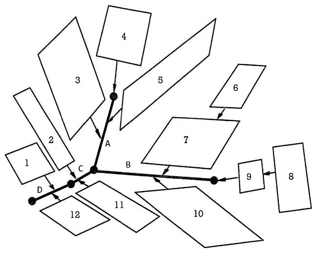
Sustainability 2020, 12, 4928                                                                       2 of 16

Soil Loss Equation (USLE) model is modified with the upslope contributing area to determine the
transport capacity function (T). In the USPED model, the divergence of the transport capacity index
(∆T) for each grid cell determines whether deposition or erosion is the dominant process. Finally,
the SEDD model was proposed by Ferro and Porto [8], although its formulation can be traced back to
Ferro and Minacapilli [9]. Based on probability, the authors of SEDD hypothesized that “the Sediment
Delivery Ratio, SDRi , of each morphological area is a measurement of the probability that the eroded
particles arrive from the considered area into the nearest stream reach” [9]. Furthermore, the authors
defined the travel time as “the time that particles eroded from the source area and transported through
the hillslope conveyance system take to arrive at the channel network” [9]. Assuming that Fi is the
cumulative distribution function (CDF) of the travel time tp,i , the authors assert that the relationship
between lnFi and tp,i is linear. Then, they support the assertion with data from seven Sicilian basins.
As a result, the following exponential function was used to describe the relationship between the SDRi
and the travel time:
                                              SDRi = e−βtp,i                                          (1)

where SDRi is the SDR of morphological unit i, β is a constant for a given basin (1/m), and tp,i is the
travel time of morphological unit i (m) and defined as:

                                                                N
                                                lp,i     Xp
                                                            λi,j
                                         tp,i = √      =    √                                          (2)
                                                  sp,i       si,j
                                                             j=1

where sp,i = the slope of the hydraulic path (m/m), lp,i = the length of the hydraulic path (m). Combining
Equations (1) and (2), SDRi can be represented as:
                                                         lp,i             PNp    λi,j
                                                     −β √s           −β          √s
                                           −βtp,i          p,i             j=1        i,j
                                 SDRi = e           =e              =e                                 (3)

where Np = the number of morphological units localized along the hydraulic path j, and λi,j and
si,j = the length (m) and slope (m/m) of each morphological unit i localized along the hydraulic path j.
       Many studies have used Equations (1)–(3) and the subsequent SDRw (SDR for the entire basin) to
estimate the movement of sediments and their impact on particular watersheds [10–14]. However,
our examination of the SEDD model led us to believe that the model might have been inadequately
formulated to represent the probability concept declared. We will show why we think so and present
our revised version of the model in the following sections.

1.2. Incorrect Assertions of SEDD
      There are several improper assumptions and false assertions of SEDD:

(a)    “the Sediment Delivery Ratio, SDRi , of each morphological area is a measurement of the probability
       that the eroded particles arrive from the considered area into the nearest stream reach” [9];
(b)    the SDRi equation is an exponential distribution (exponential probability distribution);
(c)    “the relationship between lnFi and −tp,i is linear” [9];
(d)    “the probability that the eroded particles arrive from the morphological unit into the nearest
       stream reach is assumed proportional to the probability of non-exceedance of the travel time,
       tp,i ” [9];
(e)    the β coefficient can be lumped together with “the effects due to roughness and runoff along the
       hydraulic path” [8];
(f)    the Fi is a CDF of the travel time represented by Equation (2).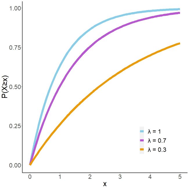
Sustainability 2020, 12, 4928                                                                          3 of 16

      It was further asserted by Ferro and Minacapilli [9] that:

                                                                   −lnFi
                                                           βi =                                           (4)
                                                                    tp,i

      These incorrect assertions will be discussed in Section 2.2.

2. Analysis
     We will start by describing the statistical properties of exponential functions and distributions,
outline the potential issues of the SEDD model, and explain how to formulate a Revised SEDD
(RSEDD) model.

2.1. Properties of Exponential Distributions
      The exponential function has a nice property concerning its differentiation and integration:

                                                           d x
                                                              ( e ) = ex                                  (5)
                                                           dx
                                                       Z
                                                               ex dx = ex + C                             (6)

where ex is the exponential function and C is a constant.
     In other words, the differentiation and integration of an exponential function is still an exponential
function. Exponential functions play a crucial role in statistical analysis. For example, if a probability
distribution takes the form of an exponential function, its probability distribution function (or probability
density function, PDF) will be an exponential distribution. The exponential distribution is generally
written as:
                                      f (x) = λe−λx x ≥ 0 and λ > 0                                       (7)

where f (x) denotes a PDF, the curve of a continuous probability distribution. Equation (7) is also called
the exponential PDF. Note the difference between exponential functions and exponential distributions.
It is also worth noting that the value f (x) is known as the probability density at x, not the probability at
x. For discrete random variables, however, relative frequency is the probability density. Unfortunately,
for continuous random variables, “it is not meaningful to associate a probability value with each
possible outcome on a continuum. Instead, for continuous random variables we associate probability
values with intervals on the continuum” [15]. For a continuous random variable, the probability at x is
zero. It is the area under the curve of a PDF that represents the probability of a variable falling in the
corresponding interval.
       The exponential distribution is a one-parameter probability distribution, which is λ. The mean of
the exponential distribution is 1/λ, and the standard deviation of the exponential distribution is also
1/λ. The exponential distribution has been applied to various fields of study, such as vehicle headway
distribution [16], the failure rates of air conditioning system in airplanes [17], the catchment-scale water
residence time [18], and the relative species abundance [19]. The cumulative distribution function
(CDF) of the exponential distribution is:
                                  Z   x                Z   x
                         F(x) =            f (u)du =           λe−λu du = 1 − e−λx x ≥ 0 and λ > 0        (8)
                                      −∞               0

where F(x) denotes a CDF (the Fi in SEDD). The PDF and CDF of the exponential distribution of typical
values of λ are shown in Figure 1a,b, respectively.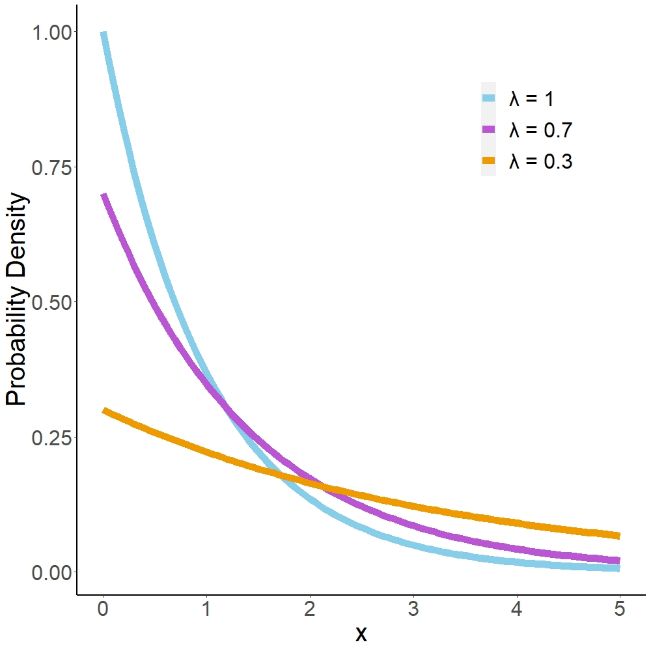
Sustainability 2020, 12, 4928 4 of 16
Sustainability 2020, 12, x FOR PEER REVIEW 4 of 16
(a) (b)
Figure
Figure 1.
1. The
The(a)
(a)probability
probabilitydistribution
distribution function
function (PDF)
(PDF) and
and the
the (b)
(b) cumulative
cumulative distribution
distribution function
function
(CDF) of the exponential distribution of typical values of λ..
(CDF) of
2.2. Examination
2.2. Examination of
of SEDD
SEDD Assertions
Assertions
The SEDD
The SEDD model
model was wasdescribed
describedininSection
Section1.1,1.1,and
andthe incorrect
the incorrect assertions
assertions were listed
were in Section
listed 1.2.
in Section
We will devote this section to discussing the issues of SEDD. We will identify
1.2. We will devote this section to discussing the issues of SEDD. We will identify the potential the potential problems
that call for
problems a revised
that call for SEDD (RSEDD)
a revised SEDDmodel to better
(RSEDD) suit the
model to underlying
better suit statistical requirements
the underlying for
statistical
modeling SDR
requirements for .
i modeling SDRi.
As mentioned earlier, using
As mentioned earlier, using morphological
morphological units,units, Ferro
Ferro andand Minacapilli
Minacapilli [9] [9] considered
considered SDR SDRii as
as
the probability that the eroded particles arrive from the source area into the
the probability that the eroded particles arrive from the source area into the nearest river channel. nearest river channel.
This seems
This seems to toimply
implythatthatthey
theyconsider
considerSDR
SDRi to be the PDF of travel time, tp,i . tOn
i to be the PDF of travel time,
the other hand, they also
p,i. On the other hand, they
wrotewrote
also that the probability
that as mentioned
the probability above is “proportional
as mentioned to the probability
above is “proportional to the of non-exceedance
probability of non-of
the travel time”. This statement seems to suggest that they consider SDR to
exceedance of the travel time.” This statement seems to suggest that they iconsider SDRi to be the CDFbe the CDF of travel time
instead.
of travel Although the Although
time instead. statementsthemight be contradictory
statements might be to each other, ittowould
contradictory not matter
each other, because
it would not
neither is correct. To formulate the relationship between SDR i and tp,i , the authors
matter because neither is correct. To formulate the relationship between SDRi and tp,i, the authors of of SEDD decided to
use an exponential function as shown in Equation (1) and repeated here as
SEDD decided to use an exponential function as shown in Equation (1) and repeated here as Equation Equation (9):
(9):
SDRi = e−βtp,i (9)
= , (9)
This is probably because of the nice properties of the exponential function (Equations (5) and (6))
This is probably because of the nice properties of the exponential function (Equations (5) and
and the fact that they needed a linear relationship (Equation (4)) between lnFi and tp,i to explain the
(6)) and the fact that they needed a linear relationship (Equation (4)) between lnFi and tp,i to explain
observed linear data from the seven Sicilian basins. However, there are a few critical problems. First,
the observed linear data from the seven Sicilian basins. However, there are a few critical problems.
the total area under a PDF has to be equal to one:
First, the total area under a PDF has to be equal to one:
Z ∞
f((x))dx =
=11 (10)
(10)
−∞
f((x)) ≥
≥ 00 for
forall
allxx (11)
(11)
Second,
Second, the
the CDF
CDF should
should be
be aa non-decreasing
non-decreasing function
function of
of xx and
and satisfy
satisfy the following equation:
the following equation:
( )=1 (12)
→
lim F(x) = 1 (12)
x→+∞
The integration of Equation (9) is:
1 1
= ( ) = = 1− = 1− , (13)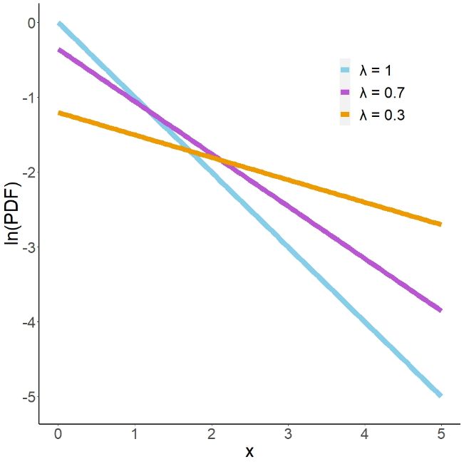
Sustainability 2020, 12, 4928                                                                                         5 of 16

      The integration of Equation (9) is:
                      Z   x             Z   x               Z         x
                                                                                        1          1
                               SDRi =           f (u)du =                 e−λu du =        1 − e−λx = 1 − e−βtp,i      (13)
                          −∞            −∞                        0                     λ            β

       Obviously, the total area under Equation (9) is not equal to one, and Equation (13) does not
approach one when x approaches infinity. Hence, Equation (9) is not a PDF. Moreover, since Equation (9)
is not a non-decreasing function, Equation (9) is not a CDF, either. As a result, we can conclude that
assertions (a), (b), (d), and (f) are incorrect.
       In addition, it can be seen that the logarithm of the CDF of Equation (9) is not linear because
Equation (13) is not a linear function. It can also be observed from Equation (13) that the integration
(i.e., CDF) of Equation (9) is not an exponential function. Therefore, a linear relationship between
lnFi and tp,i such as that in Equation (4) does not exist. The only condition that Equation (4) is valid
occurs when Equation (9) is a CDF. Since we have already shown that Equation (9) is not a CDF, we can
conclude that assertion (c) and Equation (4) are incorrect.
       Finally, the SEDD model assumes that tp,i of each morphological unit increases with the increase
of the length of the hydraulic path (lp,i ) and with the decrease of the square root of the slope of the
hydraulic path (sp,i ):
                                                 tp,i ∝ lp,i                                        (14)
                                                                      1
                                                              tp,i ∝ √                                                 (15)
                                                                      sp,i
                                                                                   √
     Therefore, there exists a constant between tp,i and the product of lp,i and 1/ sp,i . The SEDD model
lumps together the constant and the β coefficient, which changes the coefficient β from its original
meaning. Therefore, we think assertion (e) is not appropriate. We will correct these problems by
presenting the Revised SEDD (RSEDD) model in the next section.

2.3. RSEDD Model
      To distinguish from the SEDD model, we will call the following model the Revised SEDD model
(RSEDD). To comply with the statistical requirements of a probability distribution function, Equation (1)
is re-written as follows:
                                        SDRi = βe−βtp,i tp,i ≥ 0                                    (16)

      Note that β is always positive and tp,i is an exponential random variable. The CDF of Equation (16)
is the integration of Equation (16):

                                           Z             tp,i
                                   Fi = F tp,i =                  βe−βu du = 1 − e−βtp,i tp,i ≥ 0                      (17)
                                                       0

     We plot the natural logarithm of Y-axis values in Figure 2. The PDF and CDF of the exponential
distribution of typical values of λ are shown in Figure 2a,b, respectively. Note that the logarithm of
Equation (17) is not a linear function (Figure 2b). Therefore, the relationship between lnFi and tp,i is
not linear as was suggested by the SEDD model. On the contrary, Figure 2a reveals that the natural
logarithm of the exponential PDF is linear. We will use this linear property to solve for the model
parameters of RSEDD later.
     Recall that the original SEDD model assumes that tp,i of each morphological unit increases with
the increase of the ratio of the length of the hydraulic path (lp,i ) to the square root of the slope of the
hydraulic path (sp,i ). Therefore,

                                                                                lp,i
                                                                             −β √s
                                                           −βtp,i                 p,i
                                                SDRi = e                  =e             tp,i ≥ 0                      (18)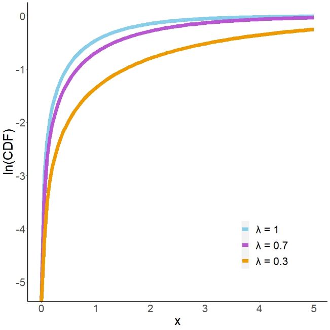
Sustainability 2020, 12, 4928 6 of 16
Sustainability 2020, 12, x FOR PEER REVIEW 6 of 16
(a) (b)
Figure
Figure 2.
2. The
The natural
natural logarithm
logarithm of of Figure
Figure 1a,b
1a,b (Y-axis
(Y-axis values
values only).
only). This
This shows
shows that
that the
the relationship
relationship
between
between ln(CDF) andttp,ip,iisisnot
ln(CDF)and notlinear
linear(Figure
(b), but2b),
thebut the relationship
relationship betweenbetween ln(PDF)
ln(PDF) and tp,iand tp,i is linear
is linear (a).
(Figure 2a).
Equation (18) holds because the SEDD model lumps together the constant between tp,i and
√
lp,i / Recall
sp,i (representing “the SEDD
that the original effects model
due to assumes
roughness and
that tp,irunoff
of eachalong the hydraulic
morphological unitpath”) the β
and with
increases
coefficient.
the increaseHowever,
of the ratio this
ofwould change
the length thehydraulic
of the β from
coefficientpath ( ,its
) tooriginal meaning.
the square We
root of will
the introduce
slope of the
a new constant
hydraulic path (k (dimensionless)
, ). Therefore, and re-write Equation (2) as follows:
,
lp,i
= ,k = = kd (18)
= tp,i (19)
√ , p,i
sp,i , ≥0
Equation (18) holds because the SEDD model lumps together the constant between tp,i and
lp,i
,⁄ , (representing “the effects due to roughness
dp,i = √ and runoff along the hydraulic path”) and (20)
the
sp,i
β coefficient. However, this would change the coefficient β from its original meaning. We will
where dp,i aisnew
introduce the pseudo
constanttravel time (m). Therefore,
k (dimensionless) and re-write Equation (2) as follows:
,l
−βtp,i ,
= −βk √p,is = , (19)
SDRi = βe = βe p,i = βe−βkdp,i d
, p,i ≥ 0 (21)
,
The rest is the same as the SEDD model. The , = exponent term has to be summed along the(20)
path
traveled by the sediments from the morphological unit , i to the nearest river. This summation is
illustrated
where dp,i isinthe
Figure 3 and
pseudo Equation
travel (22):Therefore,
time (m).
N,
lp,i X p
,
λi,j (21)
= , =√ = =√ ,
, ≥0 (22)
sp,i si,j
j=1
The rest is the same as the SEDD model. The exponent term has to be summed along the path
where Npby= the
traveled the sediments
number offrom the morphological
morphological unit i to
units localized the the
along nearest river. path
hydraulic j, and λi,j and
This summation is
si,j = the length (m) and slope (m/m) of each morphological unit i localized along the hydraulic path j.
illustrated in Figure 3 and Equation (22):
There are two parameters (β and k) of the RSEDD model as shown in Equation (21). As previously
,
shown in Figure 2, the logarithm of CDF is not linear, ,
= but the logarithm of PDF is. Therefore, to determine
(22)
the model parameters, the PDF of a basin (instead , of the CDF)
, should be used. This modification will
guarantee that the new RSEDD model is a proper depiction of the exponential distribution of travel
where Np = the number of morphological units localized along the hydraulic path j, and λi,j and si,j =
time and that SDRi is the “probability density” of the eroded particles arriving from the considered
the length (m) and slope (m/m) of each morphological unit i localized along the hydraulic path j.Sustainability 2020, 12, 4928 7 of 16
area into the nearest stream reach. To solve for model parameters β and k, take the natural logarithm of
Sustainability 2020, 12,
Equation x FOR PEER REVIEW
(21): 7 of 16
ln(SDRi ) = ln(βe−βkdp, i ) = lnβ − βkdp,i (23)
Figure 3. Illustration of the morphological unit i and the path traveled by the sediments from the
Figure 3.morphological
Illustrationunit i to the
of the nearest river in aunit
morphological basin.
i and the path traveled by the sediments fromthe
morphological unit i to the nearest river in a basin.
Equation (23) is a linear function. By plotting ln(SDRi ) against dp,i , we can determine β from the
intercept and k from the slope of the linear plot (similar to Figure 2a). In other words, given SDRi and
There are travel
pseudo two timeparameters
dp,i , we can(β and k)β of
determine andthe RSEDD
k and use RSEDDmodel as shown
to model sedimentin Equation
delivery at the (21). As
previously shown
basin scale. in Figure 2, the logarithm of CDF is not linear, but the logarithm of PDF is.
Therefore, to determine the model parameters, the PDF of a basin (instead of the CDF) should be
3. Example Watershed
used. This modification will guarantee that the new RSEDD model is a proper depiction of the
To test if the travel time follows an exponential distribution, we use a watershed from literature
exponential distribution of travel time and that SDRi is the “probability density” of the eroded
as an example [20]. Conceptually, the basin can be divided into morphological units with uniform
particlesgradients
arriving(andfrom the considered
properties) area 4.into
as shown in Figure the nearest
Assuming stream
that all units reach.
have the same To solve
gradient for model
of 0.3
parameters
and β and
that k, hydraulic
their take the paths
natural logarithm
(arrows) of Equation
are shown in Figure 5,(21):
we can calculate the slope lengths and
travel times using Figure 5 and Table 1. Note that ordinary GIS software calculates the flow lengths
ln( ) = ln( , ) = −
to the outlet of the basin, but RSEDD (SEDD) calculates the flow lengths, only to the river channels.
(23)
Here are the null hypothesis and alternative hypothesis:
Equation (23) is a linear function. By plotting ln(SDRi) against dp,i, we can determine β from the
intercept and k from the slopeH0 :of
thethe linear
travel plot
times (similar
follow to Figure
an exponential 2a). In other words, given
distribution (24)SDRi and
pseudo travel time dp,i, we can determine β and k and use RSEDD to model sediment delivery at the
basin scale. Ha : the travel times do not follow an exponential distribution (25)
3. Example Watershed
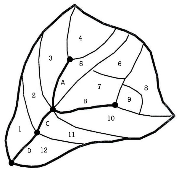
To test if the travel time follows an exponential distribution, we use a watershed from literature
as an example [20]. Conceptually, the basin can be divided into morphological units with uniform
gradients (and properties) as shown in Figure 4. Assuming that all units have the same gradient of
0.3 and that their hydraulic paths (arrows) are shown in Figure 5, we can calculate the slope lengths
and travel times using Figure 5 and Table 1. Note that ordinary GIS software calculates the flow
lengths to the outlet of the basin, but RSEDD (SEDD) calculates the flow lengths only to the riverSustainability 2020, 12, x FOR PEER REVIEW 8 of 16
Sustainability 2020, 12, 4928 8 of 16
Sustainability 2020, 12, x FOR PEER REVIEW 8 of 16
Figure 4. An example watershed (re-drawn from [20]).
Figure 4. An example watershed (re-drawn from [20]).
Figure 4. An example watershed (re-drawn from [20]).
Figure 5. Divide the sample watershed in Figure 4 into morphological units and calculate the travel
Figure 5. Divide the sample watershed in Figure 4 into morphological units and calculate the travel
times (re-drawn from [20]). The arrows indicate flow directions, and the dots correspond to the dots in
times (re-drawn
Figure 5. Divide from [20]). The
the sample arrows in
watershed indicate
Figureflow directions,
4 into and the
morphological dotsand
units correspond
calculatetothe
thetravel
dots
Figure 4.
in Figure
times 4.
(re-drawn from [20]). The arrows indicate flow directions, and the dots correspond to the dots
in Figure 4. Table 1. Pseudo travel time of each morphological area.
Table 1. Pseudo travel time of each morphological area.
λi,j
Morphological
TableUnit Hydraulic
1. Pseudo travel time of eachλi,j
Path si,j
morphological √
area.
s
i,j
dp,i
Hydraulic ,
Morphological
1 Unit 1Path 1.0 , ,
0.3 1.83 dp,i
1.83
Hydraulic ,,
Morphological
2 Unit 2 2.7, 0.3
, 4.93 dp,i
4.93
31 3Path
1 1.0
2.6 0.3
0.3 1.83
4.75, 1.83
4.75
4 12 4 12 2.7
1.0
1.6 0.3
0.3 4.93
1.83
2.92 4.93
1.83
2.92
5 23 5 23 2.6
3.9
2.7 0.3
0.3 4.75
7.12
4.93 4.75
7.12
4.93
6 34 6–7 34 1.6
1.6
2.6 0.3
0.3 2.92
2.92
4.75 6.02
2.92
4.75
7 7 1.7 0.3 3.10 3.10
45 45 3.9
1.6 0.3 7.12
2.92 7.12
2.92
8 8–9 0.9 0.3 1.64 2.92
95 6 6–7
9 5 1.6
3.9
0.7 0.3
0.3 2.92
7.12
1.28 6.02
7.12
1.28
1067 7
106–7 1.7
1.6
2.6 0.3
0.3 3.10
2.92
4.75 3.10
6.02
4.75
1178 118–9
7 2.1
0.9
1.7 0.3
0.3 3.83
1.64
3.10 3.83
2.92
3.10
1289 128–9
9 1.3
0.7
0.9 0.3
0.3 2.37
1.28
1.64 2.37
1.28
2.92
10
9 10
9 2.6
0.7 0.3 4.75
1.28 4.75
1.28
11
10
We used the Kolmogorov-Smirnov 11
test in 10 2.1 hypothesis
2.6
our statistical 0.3 3.83
4.75
testing. 3.83
4.75
Reordering the dp,i in
12
Table 1 from the smallest11 to the largest, we can 12calculate2.1
11 1.3 0.3
the cumulative 2.37
3.83 2.37 of our sample
3.83
distribution
12
watershed and the corresponding cumulative12 distribution1.3of the0.3 2.37 distribution
exponential 2.37 as shown
We used the Kolmogorov-Smirnov test in our statistical hypothesis testing. Reordering the dp,i
in Table 2. For a confidence coefficient (1–α) of 0.95, we obtained the sample statistic of 0.213 (Dn ).
in Table
We 1used
fromthe
theKolmogorov-Smirnov
smallest to the largest,test
wein can calculate
our thehypothesis
statistical cumulativetesting.
distribution of our sample
Reordering the dp,i
in Table 1 from the smallest to the largest, we can calculate the cumulative distribution of our sampleSustainability 2020, 12, 4928 9 of 16
Since Dn is not greater than the critical value of 0.375 (D12,0.05 ), we cannot reject the null hypothesis (H0 )
that these data come from an exponential distribution. However, we cannot accept the null hypothesis
(H0 ) either because we only know a Type I error (probability equal to α = 0.05) and do not know
the probability of making a Type II error [21]. The hypothesis testing on this example watershed is
not conclusive.
Table 2. Results of the Kolmogorov-Smirnov test.
x Frequency Cumulative Cumulative (%) Corresponding Exponential CDF (%) Difference
1.28 1 1 0.083 0.284 0.201
1.83 1 2 0.167 0.380 0.213
2.37 1 3 0.250 0.463 0.213
2.92 1 4 0.333 0.535 0.201
2.92 1 5 0.417 0.535 0.118
3.10 1 6 0.500 0.556 0.056
3.83 1 7 0.583 0.634 0.050
4.75 1 8 0.667 0.711 0.045
4.75 1 9 0.750 0.711 0.039
4.93 1 10 0.833 0.725 0.108
6.02 1 11 0.917 0.794 0.123
7.12 1 12 1.000 0.845 0.155
Total 12
Mean 3.82 Dn 0.213
λ 0.262 D12,0.05 0.375
4. Discussion
The original studies of the SEDD model preceded several studies evaluating SDR, and its impact
on geomorphology and other related issues was far-reaching. Therefore, a revision to the model
would have an impact on the conclusions of some (but not all) of the publications which cited the
original model. There are two different categories of impacts we have ascertained from our literature
review: (a) foundation research that established and confirmed the SEDD model and validated the
use of the model, and (b) studies which merely mention the SEDD model without implementation.
The first category is strongly impacted by the revision of SEDD, while the revision has no impact on
the second category.
The first collection of studies are studies that established, tested, and calibrated the SEDD model
parameters (or its offsets, such as MOSEDD) and those studies in which SEDD plays a significant role
in the procedure of the research. The first type of studies established that although there were many
different gross erosion estimation models (RUSLE, USLE, USLE-M, USLE-MM, etc.), the SDR of the
SEDD model was conceptually practical for estimating the sediment yield. Therefore, the specific
gross erosion model considered was not particularly influential. The conclusions of these studies
would require recalibration as the base model would be changed. However, the separation of the
physical concept of sediment delivery and the SEDD from the gross erosion estimation concept remains
intact. Alternatively, the second type of study used the SEDD model as a significant component.
The conclusions and results would need to be re-evaluated to see the extent of the impact due to the
use of a new model. These studies and their contributions are as follows: the relationship between
channel network parameters and the sediment transport efficiency [22], the testing and calibration of
the SEDD model [8,23–28], the assessment of sediment connectivity in dendritic and parallel Calanchi
systems [29,30], sediment load impact on a reservoir [14], the estimation of the response to land
use/cover change in a catchment [31], sediment yield in monocrop plantation areas, such as reafforested
eucalyptus and olive orchards [13,32], the assessment of sediment delivery/soil erosion processes using
Caesium-137 [23,33–37], testing of the correction of the topographic factors of the RUSLE [38–42],
soil erosion and sediment yield estimation [10,43–58], agricultural non-point pollution [59], clay content
relationship with sediment delivery [60], the assessment of the temporal variation of sediment yield [61],
chemical transport in sediment delivery processes [62,63], agricultural methods impact on soil erosion
and sediment yield [11,12], impact of bushfire or wildfire on soil erosion [64], comparison of multipleSustainability 2020, 12, 4928 10 of 16
SDR models/gross erosion models [65,66], soil texture prediction [67], relating geomorphic features
to soil erosion [68], landscape management and water resources management [69], and land use and
impact of check dams on sediment yield [70–72].
Many studies have cited the conclusions or observations made by Ferro and Minacapilli [9] and
the SEDD model within their literature review. However, they have not explicitly employed the
SEDD model or the SDR equation. These represent the second collection of studies related to the
SEDD model. Common citations are for the following reasons: (1) as an example of research which
uses RUSLE, (2) travel time as a basis for the regionalization of SDR, (3) defining SDR, (4) sediment
transport and its relationship with storage time and the sediment delivery ratio, (5) lumped sediment
delivery ratio, (6) linkage between different scales using the SDR equation, (7) empirical models to
evaluate sediment yield and soil erosion, (8) sediment yield being proportional to the sediment delivery
processes, (9) topographic factors and their relationship with SDR, (10) spatially distributed empirical
erosion models, and (11) calibration of measured and calculated sediment yields [2,68,73–129].
The preceding literature review includes all accessible papers to the authors of this study (using the
Scopus database). It confirms that between 1995, the year the SEDD model was published, to 2019,
there has been no revision of the SEDD model similar to what is proposed in this study. Note that
there might be additional studies that have not been included in the literature review of this study
because these papers utilized the SEDD model but did not reference the original study of the SEDD
model [9]. For example, Diwediga et al. [130] utilized the SEDD model to study soil erosion response to
sustainable land management in the Mo River Basin, Togo, Africa, but referenced the Di Stefano et al. [36]
equation instead. Finally, the great influence the original paper on sediment delivery research over the
past 25 years gives rise to an innumerable number of references. These references might exist in less
accessible databases, conference materials, and in national/state/municipal level public research that are
beyond our ability to review.
5. Summary and Conclusions
Using exponential distributions to model naturally occurring phenomena is quite common in
natural science and engineering analysis. The use of exponential distribution to model the probability
of sediments entering river channels is an essential contribution of SEDD, and the model has been
widely used to study different basins in the world. However, there are several false assertions by the
SEDD model, which do not seem to have been noticed in the literature. We reviewed this often used
model and proposed to revise it to better suit the underlying statistical requirements. As a result,
the RSEDD model was introduced with two model parameters, β and k. The calibration of these
parameters can be done using the logarithm of PDF. We also reviewed literature citing the SEDD
model to see the impact of the revision on these studies. The first collection of studies are studies that
calibrated the SEDD model parameters or used the SEDD model as a significant component of the
studies. These studies need to be re-evaluated to see the extent of the impact. The second collection of
studies used the SEDD model as an example or merely mentioned the model without implementation.
The revision does not affect these studies. However, it remains to be seen whether the new RSEDD
model can reliably predict SDRi and sediment yield in future watershed research.
Author Contributions: Conceptualization, W.C.; Data curation, K.T.; Formal analysis, W.C.; Funding acquisition,
W.C.; Investigation, W.C. and K.T.; Methodology, W.C.; Project administration, W.C.; Resources, W.C.; Software,
K.T.; Supervision, W.C.; Writing—original draft, W.C. and K.T.; Writing—review & editing, W.C. All authors have
read and agreed to the published version of the manuscript.
Funding: This study was partially supported by the National Taipei University of Technology-King Mongkut’s
Institute of Technology Ladkrabang Joint Research Program (Grant Number NTUT-KMITL-108-01) and the
Ministry of Science and Technology (Taiwan) Research Project (Grant Number MOST 108-2621-M-027-001).
Acknowledgments: We thank Kieu Anh Nguyen, Chih-Hung Wang, and Tse-Wei Lo for assistance with manuscript
preparation. We also thank the anonymous reviewers for their careful reading of our manuscript and insightful
suggestions to improve the paper.
Conflicts of Interest: The authors declare no conflict of interest.Sustainability 2020, 12, 4928 11 of 16
References
1. Van Oost, K.; Govers, G.; Desmet, P. Evaluating the effects of changes in landscape structure on soil erosion
by water and tillage. Landsc. Ecol. 2000, 15, 577–589. [CrossRef]
2. Van Rompaey, A.J.J.; Verstraeten, G.; Van Oost, K.; Govers, G.; Poesen, J. Modelling mean annual sediment
yield using a distributed approach. Earth Surf. Proc. Landf. 2001, 26, 1221–1236. [CrossRef]
3. Verstraeten, G.; Van Oost, K.; Van Rompaey, A.; Poesen, J.; Govers, G. Evaluating an integrated approach to
catchment management to reduce soil loss and sediment pollution through modelling. Soil Use Manag. 2002,
18, 386–394. [CrossRef]
4. Mitasova, H.; Hofierka, J.; Zlocha, M.; Iverson, L.R. Modeling topographic potential for erosion and deposition
using GIS. Int. J. Geogr. Inf. Syst. 1996, 10, 629–641. [CrossRef]
5. Mitas, L.; Mitasova, H. Distributed soil erosion simulation for effective erosion prevention. Water Resour. Res.
1998, 34, 505–516. [CrossRef]
6. Mitasova, H.; Mitas, L. Multiscale soil erosion simulations for land use management. In Landscape Erosion and
Landscape Evolution Modeling; Harmon, R., Doe, W.W., Eds.; Springer: New York, NY, USA, 2001; pp. 321–348.
7. Warren, S.D.; Mitášová, H.; Hohmann, M.G.; Landsberger, S.; Iskander, F.Y.; Ruzycki, T.S.; Senseman, G.M.
Validation of a 3-D enhancement of the Universal Soil Loss Equation for prediction of soil erosion and
sediment deposition. Catena 2005, 64, 281–296. [CrossRef]
8. Ferro, V.; Porto, P. Sediment delivery distributed (SEDD) model. J. Hydrol. Eng. 2000, 5, 411–422. [CrossRef]
9. Ferro, V.; Minacapilli, M. Sediment delivery processes at basin scale. Hydrol. Sci. J. 1995, 40, 703–717. [CrossRef]
10. Fernandez, C.; Wu, J.Q.; McCool, D.K.; Stöckle, C.O. Estimating water erosion and sediment yield with GIS,
RUSLE, and SEDD. J. Soil Water Conserv. 2003, 58, 128–136.
11. Fu, G.; Chen, S.; McCool, D.K. Modeling the impacts of no-till practice on soil erosion and sediment yield
with RUSLE, SEDD, and ArcView GIS. Soil Tillage Res. 2006, 85, 38–49. [CrossRef]
12. Tanyaş, H.; Kolat, Ç.; Süzen, M.L. A new approach to estimate cover-management factor of RUSLE and
validation of RUSLE model in the watershed of Kartalkaya Dam. J. Hydrol. 2015, 528, 584–598. [CrossRef]
13. Burguet, M.; Taguas, E.V.; Gómez, J.A. Exploring calibration strategies of the SEDD model in two olive
orchard catchments. Geomorphology 2017, 290, 17–28. [CrossRef]
14. Olii, M.R.; Kironoto, B.A.; Yulistiyanto, B.; Sunjoto, S. Estimating spatially distributed of sediment yield
using GIS-RUSLE-SEDD model in catchment of reservoir in Java. In Multi-Perspective Water for Sustainable
Development, Proceedings of the 21st International Association for Hydro-Environment Engineering and Research-Asia
Pacific Division (IAHR-APD) Congress, Yohyakarta, Indonesia, 2–5 September 2018; IAHR-APD: Gyeonggi-Do,
Korea, 2018; pp. 351–358.
15. Neter, J.; Wasserman, W.; Whitmore, G.A. Applied Statistics, 4th ed.; Allyn and Bacon: Boston, MA, USA,
1993; pp. 153–155.
16. Zhang, G.; Wang, Y.; Wei, H.; Chen, Y. Examining headway distribution models with urban freeway loop
event data. Transp. Res. Rec. 2007, 1999, 141–149. [CrossRef]
17. Proschan, F. Theoretical explanation of observed decreasing failure rate. Technometrics 2000, 42, 7–11. [CrossRef]
18. McGuire, K.J.; McDonnell, J.J.; Weiler, M.; Kendall, C.; McGlynn, B.L.; Welker, J.M.; Seibert, J. The role of
topography on catchment-scale water residence time. Water Resour. Res. 2005, 41, 1–14. [CrossRef]
19. Shipley, B.; Vile, D.; Garnier, É. From plant traits to plant communities: A statistical mechanistic approach to
biodiversity. Science 2006, 314, 812–814. [CrossRef] [PubMed]
20. Morgan, R.P.C.; Quinton, J.N.; Smith, R.E.; Govers, G.; Poesen, J.W.A.; Auerswald, K.; Chisci, G.; Torri, D.;
Styczen, M.E.; Folly, A.J.V. The European Soil Erosion Model (EUROSEM): Documentation and User Guide;
Silsoe College, Cranfield University: Bedford, UK, 1998; pp. 35–36.
21. Mendenhall, W.; Sincich, T. A Second Course in Business Statistics: Regression Analysis, 3rd ed.; Dellen Publishing
Company: San Francisco, CA, USA, 1989; pp. 37–40.
22. Ferro, V. Further remarks on a distributed approach to sediment delivery. Hydrol. Sci. J. 1997, 42, 633–647. [CrossRef]
23. Ferro, V.; Porto, P.; Tusa, G. Testing a distributed approach for modelling sediment delivery. Hydrol. Sci. J.
1998, 43, 425–442. [CrossRef]Sustainability 2020, 12, 4928 12 of 16
24. Ferro, V.; Di Stefano, C.; Minacapilli, M.; Santoro, M. Calibrating the SEDD model for Sicilian ungauged basins.
In Erosion Prediction in Ungauged Basins: Integrating Methods and Techniques, Proceedings of the Symposium HS01
Held During International Union of Geodesy and Geophysics (IUGG) 2003, Sapporo, Japan, 30 June–11 July 2003;
IAHS-AISH Publication: Wallingford, Oxfordshire, UK, 2003; Volume 279, pp. 151–161.
25. Di Stefano, C.; Ferro, V.; Minacapilli, M. Testing the SEDD model in Sicilian basins. In Sediment. Budgets 2,
Proceedings of the Symposium S1 Held during the Seventh International Association of Hydrological Sciences (IAHS)
Scientific Assembly, Foz do Iguaçu, Brazil, 3–9 April 2005; IAHS-AISH Publication: Wallingford, Oxfordshire,
UK, 2005; Volume 292, pp. 152–161.
26. Di Stefano, C.; Ferro, V. Testing the Modified Sediment Delivery Model (MOSEDD) at SPA2 Experimental
Basin, Sicily (Italy). Land Degrad. Dev. 2017, 28, 1557–1567. [CrossRef]
27. Di Stefano, C.; Ferro, V. Testing Sediment Connectivity at the Experimental SPA2 Basin, Sicily (Italy).
Land Degrad. Dev. 2017, 28, 1992–2000. [CrossRef]
28. Di Stefano, C.; Ferro, V. Modelling sediment delivery using connectivity components at the experimental
SPA2 basin, Sicily (Italy). J. Mt. Sci. 2018, 15, 1868–1880. [CrossRef]
29. Di Stefano, C.; Ferro, V. Assessing sediment connectivity in dendritic and parallel calanchi systems.
Catena 2019, 172, 647–654. [CrossRef]
30. Caraballo-Arias, N.A.; Di Stefano, C.; Ferro, V. Morphological characterization of calanchi (badland) hillslope
connectivity. Land Degrad. Dev. 2018, 29, 1190–1197. [CrossRef]
31. Yan, R.; Zhang, X.; Yan, S.; Chen, H. Estimating soil erosion response to land use/cover change in a catchment
of the Loess Plateau, China. Int. Soil Water Conserv. Res. 2018, 6, 13–22. [CrossRef]
32. Porto, P.; Cogliandro, V.; Callegari, G. Exploring the performance of the SEDD model to predict sediment yield
in eucalyptus plantations. Long-term results from an experimental catchment in Southern Italy. In Institute
of Physics (IOP) Conference Series: Earth and Environmental Science, Proceedings of the 3rd International Conference
Environment and Sustainable Development of Territories: Ecological Challenges of the 21st Century, Kazan, Russia,
27–29 September 2017; IOP Publishing: Bristol, UK, 2018; Volume 107.
33. Di Stefano, C.; Ferro, V.; Porto, P. Linking sediment yield and caesium-137 spatial distribution at basin scale.
J. Agric. Eng. Res. 1999, 74, 41–62. [CrossRef]
34. Di Stefano, C.; Ferro, V.; Rizzo, S. Assessing soil erosion in a small Sicilian basin by caesium-137 measurements
and a simplified mass balance model. Hydrol. Sci. J. 2000, 45, 817–832. [CrossRef]
35. He, Q.; Walling, D.E. Testing distributed soil erosion and sediment delivery models using 137Cs measurements.
Hydrol. Proc. 2003, 17, 901–916. [CrossRef]
36. Di Stefano, C.; Ferro, V.; Porto, P.; Rizzo, S. Testing a spatially distributed sediment delivery model (SEDD)
in a forested basin by cesium-137 technique. J. Soil Water Conserv. 2005, 60, 148–157.
37. Porto, P.; Walling, D.E. Use of caesium-137 measurements and long-term records of sediment load to calibrate
the sediment delivery component of the SEDD model and explore scale effect: Examples from southern Italy.
J. Hydrol. Eng. 2015, 20. [CrossRef]
38. Di Stefano, C.; Ferro, V.; Porto, P. Modelling sediment delivery processes by a stream tube approach.
Hydrol. Sci. 1999, 44, 725–742. [CrossRef]
39. Di Stefano, C.; Ferro, V.; Porto, P. Length slope factors for applying the revised universal soil loss equation at
basin scale in southern Italy. J. Agric. Eng. Res. 2000, 75, 349–364. [CrossRef]
40. Di Stefano, C.; Ferro, V.; Porto, P.; Tusa, G. Slope curvature influence on soil erosion and deposition processes.
Water Resour. Res. 2000, 36, 607–617. [CrossRef]
41. Zhao, Z.; Thien, L.C.; Yang, Q.; Rees, H.W.; Benoy, G.; Xing, Z.; Meng, F.-R. Model prediction of soil drainage
classes based on digital elevation model parameters and soil attributes from coarse resolution soil maps.
Can. J. Soil Sci. 2008, 88, 787–799. [CrossRef]
42. Vigiak, O.; Borselli, L.; Newham, L.T.H.; McInnes, J.; Roberts, A.M. Comparison of conceptual landscape
metrics to define hillslope-scale sediment delivery ratio. Geomorphology 2012, 138, 74–88. [CrossRef]
43. Jain, M.K.; Kothyari, U.C. Estimation of soil erosion and sediment yield using GIS. Hydrol. Sci. 2000, 4,
771–786. [CrossRef]
44. Son, K.I.; Lee, J.J. Prediction of erosion and deposition in a mountainous basin. In Sediment. Budgets 2,
Proceedings of Symposium S1 Held during the Seventh International Association of Hydrological Sciences (IAHS)
Scientific Assembly, Foz do Iguaçu, Brazil, 3–9 April 2005; IAHS-AISH Publication: Wallingford, Oxfordshire,
UK, 2005; Volume 292, pp. 152–161, 185–193.Sustainability 2020, 12, 4928 13 of 16
45. Mutua, B.M.; Klik, A.; Loiskandl, W. Modelling soil erosion and sediment yield at a catchment scale: The case
of Masinga catchment, Kenya. Land Degrad. Dev. 2006, 17, 557–570. [CrossRef]
46. Di Stefano, C.; Ferro, V. Evaluation of the SEDD model for predicting sediment yield at the Sicilian
experimental SPA2 basin. Earth Surf. Proc. Landf. 2007, 32, 1094–1109. [CrossRef]
47. Bhattarai, R.; Dutta, D. Estimation of soil erosion and sediment yield using GIS at catchment scale. Water Resour.
Manag. 2007, 21, 1635–1647. [CrossRef]
48. Drzewiecki, W.; Mularz, S. Simulation of water soil erosion effects on sediment delivery to Dobczyce
Reservoir. Int. Arch. Photogramm. Remote Sens. Spat. Inf. Sci.—ISPRS Arch. 2008, 37, 787–794.
49. Vigiak, O.; Newham, L.T.H.; Whitford, J.; Melland, A.; Borselli, L. Comparison of landscape approaches to
define spatial patterns of hillslope-scale sediment delivery ratio. In I14. Biophysical Modelling to Prioritise
Catchment Management Effort, Proceedings of the 18th World IMACS Congress and MODSIM09 International
Congress on Modelling and Simulation. Modelling and Simulation Society of Australia and New Zealand and
International Association for Mathematics and Computers in Simulation, Cairns, Australia, 13–17 July 2009;
Anderssen, R.S., Braddock, R.D., Newham, L.T.H., Eds.; Modelling and Simulation Society of Australia and
New Zealand (MSSANZ): Canberra, Australia, 2009; pp. 4064–4070.
50. Ali, K.F.; De Boer, D.H. Spatially distributed erosion and sediment yield modeling in the upper Indus River
basin. Water Resour. Res. 2010, 46. [CrossRef]
51. Chen, L.; Qian, X.; Shi, Y. Critical Area Identification of Potential Soil Loss in a Typical Watershed of the
Three Gorges Reservoir Region. Water Resour. Manag. 2011, 25, 3445–3463. [CrossRef]
52. Capra, A.; Ferro, V.; Porto, P.; Scicolone, B. Quantifying interrill and ephemeral gully erosion in a small
Sicilian basin. Z. Geomorphol. 2012, 56 (Suppl. 1), 9–25. [CrossRef]
53. Saygın, S.D.; Ozcan, A.U.; Basaran, M.; Timur, O.B.; Dolarslan, M.; Yılman, F.E.; Erpul, G. The combined
RUSLE/SDR approach integrated with GIS and geostatistics to estimate annual sediment flux rates in the
semi-arid catchment, Turkey. Environ. Earth Sci. 2014, 71, 1605–1618. [CrossRef]
54. Lee, S.E.; Kang, S.H. Geographic information system-coupling sediment delivery distributed modeling based
on observed data. Water Sci. Technol. 2014, 70, 495–501. [CrossRef] [PubMed]
55. Kang, S.H. GIS-based sediment transport in Asian monsoon region. Environ. Earth Sci. 2014, 73, 221–230. [CrossRef]
56. Pohlert, T. Projected climate change impact on soil erosion and sediment yield in the river Elbe catchment.
In Sediment Matters; Heininger, P., Cullmann, J., Eds.; Springer International Publishing: Cham, Switzerland,
2015; pp. 97–108.
57. Taguas, E.V.; Guzmán, E.; Guzmán, G.; Vanwalleghem, T.; Gómez, J.A. Characteristics and importance of
rill and gully erosion: A case study in a small catchment of a marginal olive grove. Cuadernos Investigacion
Geografica 2015, 41, 107–126. [CrossRef]
58. Batista, P.V.G.; Silva, M.L.N.; Silva, B.P.C.; Curi, N.; Bueno, I.T.; Acérbi Júnior, F.W.; Davies, J.; Quinton, J.
Modelling spatially distributed soil losses and sediment yield in the upper Grande River Basin—Brazil.
Catena 2017, 157, 139–150. [CrossRef]
59. Di Stefano, C.; Ferro, V.; Palazzolo, E.; Panno, M. Sediment delivery processes and agricultural non-point
pollution in a Sicilian Basin. J. Agric. Eng. Res. 2000, 77, 103–112. [CrossRef]
60. Di Stefano, C.; Ferro, V. Linking clay enrichment and sediment delivery processes. Biosyst. Eng. 2002, 81,
465–479. [CrossRef]
61. Kothyari, U.C.; Jain, M.K.; Ranga Raju, K.G. Estimation of temporal variation of sediment yield using GIS.
Hydrol. Sci. 2002, 47, 693–706. [CrossRef]
62. Di Stefano, C.; Ferro, V.; Palazzolo, E.; Panno, M. Sediment delivery processes and chemical transport in a
small forested basin. Hydrol. Sci. 2005, 50, 697–712. [CrossRef]
63. Huang, J.; Li, Q.; Tu, Z.; Pan, C.; Zhang, L.; Ndokoye, P.; Lin, J.; Hong, H. Quantifying land-based pollutant
loads in coastal area with sparse data: Methodology and application in China. Ocean Coast. Manag. 2013, 81,
14–28. [CrossRef]
64. Di Piazza, G.V.; Di Stafano, C.; Ferro, V. Modelling the effects of a bushfire on erosion in a Mediterranean
basin. Hydrol. Sci. 2007, 52, 1253–1270. [CrossRef]
65. Kinsey-Henderson, A.E.; Post, D.A. Evaluation of the scale dependence of a spatially-explicit hillslope
sediment delivery ratio model. In Proceedings of the 3rd International Congress on Environmental Modelling
and Software (iEMSs), Burlington, VT, USA, 1 July 2006; BYU ScholarsArchive: Provo, UT, USA, 2006; p. 213.Sustainability 2020, 12, 4928 14 of 16
66. Post, D.A.; Kinsey-Henderson, A.E.; Bartley, R.; Hawdon, A. Deriving a spatially-explicit hillslope sediment
delivery ratio model based on the travel time of water across a hillslope. In Proceedings of the 3rd
International Congress on Environmental Modelling and Software (iEMSs), Burlington, VT, USA, 1 July 2006;
BYU ScholarsArchive: Provo, UT, USA, 2006; p. 213.
67. Zhao, Z.; Chow, T.L.; Rees, H.W.; Yang, Q.; Xing, Z.; Meng, F.-R. Predict soil texture distributions using an
artificial neural network model. Comput. Electron. Agric. 2009, 65, 36–48. [CrossRef]
68. López-Vicente, M.; Navas, A. Relating soil erosion and sediment yield to geomorphic features and erosion
processes at the catchment scale in the Spanish Pre-Pyrenees. Environ. Earth Sci. 2010, 61, 143–158. [CrossRef]
69. Tamene, L.; Le, Q.B.; Vlek, P.L.G. A Landscape Planning and Management Tool for Land and Water Resources
Management: An Example Application in Northern Ethiopia. Water Resour. Manag. 2014, 28, 407–424. [CrossRef]
70. Zhao, G.; Kondolf, G.M.; Mu, X.; Han, M.; He, Z.; Rubin, Z.; Wang, F.; Gao, P.; Sun, W. Sediment yield
reduction associated with land use changes and check dams in a catchment of the Loess Plateau, China.
Catena 2017, 148, 126–137. [CrossRef]
71. Tamene, L.; Adimassu, Z.; Aynekulu, E.; Yaekob, T. Estimating landscape susceptibility to soil erosion using
a GIS-based approach in Northern Ethiopia. Int. Soil Water Conserv. Res. 2017, 5, 221–230. [CrossRef]
72. Xu, Y.; Tang, H.; Wang, B.; Chen, J. Effects of landscape patterns on soil erosion processes in a mountain–basin
system in the North China. Nat. Hazard. 2017, 87, 1567–1585. [CrossRef]
73. Walling, D.E.; He, Q. Use of fallout 137Cs measurements for validating and calibrating soil erosion and
sediment delivery models. IAHS-AISH Publ. 1998, 249, 267–278.
74. De Roo, A.P.J. Modelling runoff and sediment transport in catchments using GIS. Hydrol. Proc. 1998, 12,
905–922. [CrossRef]
75. Di Stefano, C.; Ferro, V.; Porto, P. Applying the bootstrap technique for studying soil redistribution by
caesium-137 measurements at basin scale. Hydrol. Sci. 2000, 45, 171–183. [CrossRef]
76. Lu, X.X.; Higgitt, D.L. Sediment delivery to the Three Gorges 2: Local response. Geomorphology 2001, 41,
157–169. [CrossRef]
77. Prosser, I.P.; Rutherfurd, I.D.; Olley, J.M.; Young, W.J.; Wallbrink, P.J.; Moran, C.J. Large-scale patterns of
erosion and sediment transport in river networks, with examples from Australia. Mar. Freshw. Res. 2001, 52,
81–99. [CrossRef]
78. Merritt, W.S.; Letcher, R.A.; Jakeman, A.J. A review of erosion and sediment transport models. Environ. Model.
Softw. 2003, 18, 761–799. [CrossRef]
79. Kaur, R.; Singh, O.; Srinivasan, R.; Das, S.N.; Mishra, K. Comparison of a subjective and a physical approach
for identification of priority areas for soil and water management in a watershed—A case study of Nagwan
watershed in Hazaribagh District of Jharkhand, India. Environ. Model. Assess. 2004, 9, 115–127. [CrossRef]
80. Phillips, J.D.; Slattery, M.C.; Musselman, Z.A. Dam-to-delta sediment inputs and storage in the lower trinity
river, Texas. Geomorphology 2004, 62, 17–34. [CrossRef]
81. Amore, E.; Modica, C.; Nearing, M.A.; Santoro, V.C. Scale effect in USLE and WEPP application for soil
erosion computation from three Sicilian basins. J. Hydrol. 2004, 293, 100–114. [CrossRef]
82. Scanlon, T.M.; Kiely, G.; Xie, Q. A nested catchment approach for defining the hydrological controls on
non-point phosphorus transport. J. Hydrol. 2004, 291, 218–231. [CrossRef]
83. Lu, H.; Moran, C.J.; Sivapalan, M. A theoretical exploration of catchment-scale sediment delivery. Water Resour.
Res. 2005, 41, 1–15. [CrossRef]
84. Parsons, A.J.; Wainwright, J.; Brazier, R.E.; Powell, D.M. Is sediment delivery a fallacy? Earth Surf. Proc.
Landf. 2006, 31, 1325–1328. [CrossRef]
85. Verstraeten, G.; Prosser, I.P.; Fogarty, P. Predicting the spatial patterns of hillslope sediment delivery to river
channels in the Murrumbidgee catchment, Australia. J. Hydrol. 2007, 334, 440–454. [CrossRef]
86. Grauso, S.; Pagano, A.; Fattoruso, G.; De Bonis, P.; Onori, F.; Regina, P.; Tebano, C. Relations between
climatic-geomorphological parameters and sediment yield in a mediterranean semi-arid area (Sicily, Southern
Italy). Environ. Geol. 2008, 54, 219–234. [CrossRef]
87. Lu, H.; Richards, K. Sediment delivery: New approaches to modelling an old problem. In River Confluences,
Tributaries and the Fluvial Network; Rice, S.P., Roy, A.G., Rhoads, B.L., Eds.; John Wiley & Sons Ltd.: Chichester,
UK, 2008; pp. 337–366.
88. Krishna Bahadur, K.C. Mapping soil erosion susceptibility using remote sensing and GIS: A case of the
Upper Nam Wa Watershed, Nan Province, Thailand. Environ. Geol. 2009, 57, 695–705. [CrossRef]Sustainability 2020, 12, 4928 15 of 16
89. Ding, J.; Richards, K. Preliminary modelling of sediment production and delivery in the Xihanshui River
basin, Gansu, China. Catena 2009, 79, 277–287. [CrossRef]
90. Verstraeten, G.; Rommens, T.; Peeters, I.; Poesen, J.; Govers, G.; Lang, A. A temporarily changing Holocene
sediment budget for a loess-covered catchment (central Belgium). Geomorphology 2009, 108, 24–34. [CrossRef]
91. Higgitt, D. Continental-scale river basins. In Sediment Cascades: An Integrated Approach; Burt, T.P., Allison, R.J.,
Eds.; John Wiley & Sons, Ltd.: Chichester, UK, 2009; p. 397.
92. Zhao, Z.; Yang, Q.; Benoy, G.; Chow, T.L.; Xing, Z.; Rees, H.W.; Meng, F.-R. Using artificial neural network
models to produce soil organic carbon content distribution maps across landscapes. Can. J. Soil Sci. 2010, 90,
75–87. [CrossRef]
93. Alatorre, L.C.; Beguería, S.; García-Ruiz, J.M. Regional scale modeling of hillslope sediment delivery:
A case study in the Barasona Reservoir watershed (Spain) using WATEM/SEDEM. J. Hydrol. 2010, 391,
109–123. [CrossRef]
94. Arekhi, S.; Shabani, A.; Alavipanah, S.K. Evaluation of integrated KW-GIUH and MUSLE models to predict
sediment yield using geographic information system (GIS) (Case study: Kengir watershed, Iran). Afr. J.
Agric. Res. 2011, 6, 4185–4198.
95. Hicks, D.M.; Shankar, U.; Mckerchar, A.I.; Basher, L.; Lynn, I.; Page, M.; Jessen, M. Suspended sediment
yields from New Zealand rivers. J. Hydrol. N. Z. 2011, 50, 81–142.
96. Walling, D.E.; Wilkinson, S.H.; Horowitz, A.J. Catchment erosion, sediment delivery, and sediment quality.
In Treatise on Water Science; Wilderer, P., Rogers, P., Uhlenbrook, S., Frimmel, F., Hanaki, K., Vereijken, T., Eds.;
Elsevier: Amsterdam, The Netherlands, 2011; Volume 2, p. 322.
97. Grismer, M.E. Erosion modelling for land management in the Tahoe basin, USA: Scaling from plots to forest
catchments. Hydrol. Sci. 2012, 57, 878–900. [CrossRef]
98. Chowdary, V.M.; Chakraborthy, D.; Jeyaram, A.; Murthy, Y.V.N.K.; Sharma, J.R.; Dadhwal, V.K. Multi-Criteria
Decision Making Approach for Watershed Prioritization Using Analytic Hierarchy Process Technique and
GIS. Water Resour. Manag. 2013, 27, 3555–3571. [CrossRef]
99. Park, W.S.; Hong, S.H.; Hwan, A.C.; Hyun, C. Assessment of soil loss in irrigation reservoir based on GIS.
J. Korean Soc. Surv. Geod. Photogramm. Cartogr. 2013, 31, 439–446. [CrossRef]
100. Zhao, Z.; MacLean, D.A.; Bourque, C.P.-A.; Swift, D.E.; Meng, F.-R. Generation of soil drainage equations
from an artificial neural network-analysis approach. Can. J. Soil Sci. 2013, 93, 329–342. [CrossRef]
101. Wu, L.; Long, T.-Y.; Liu, X.; Ma, X.-Y. Modeling impacts of sediment delivery ratio and land management
on adsorbed non-point source nitrogen and phosphorus load in a mountainous basin of the Three Gorges
reservoir area, China. Environ. Earth Sci. 2013, 70, 1405–1422. [CrossRef]
102. Son, K.-I.; Woo, K.-S.; Kang, Y.-G.; Kim, K.-M.; Son, G.-C. Characteristics of nonpoint source erosion from
burned mountain basin. Adv. Mater. Res. 2013, 610, 2787–2790. [CrossRef]
103. Dumitriu, D. Source area lithological control on sediment delivery ratio in Trotuş drainage basin
(Eastern Carpathians). Geogr. Fisica Din. Quat. 2014, 37, 91–100.
104. Karydas, C.G.; Panagos, P.; Gitas, I.Z. A classification of water erosion models according to their geospatial
characteristics. Int. J. Digit. Earth 2014, 7, 229–250. [CrossRef]
105. Kim, S.M.; Jang, T.I.; Kang, M.S.; Im, S.J.; Park, S.W. GIS-based lake sediment budget estimation taking into
consideration land use change in an urbanizing catchment area. Environ. Earth Sci. 2014, 71, 2155–2165. [CrossRef]
106. Zheng, M.; Liao, Y.; He, J. Sediment delivery ratio of single flood events and the influencing factors in a
headwater basin of the Chinese loess plateau. PLoS ONE 2014, 9, e112594. [CrossRef]
107. Bezak, N.; Rusjan, S.; Petan, S.; Sodnik, J.; Mikoš, M. Estimation of soil loss by the WATEM/SEDEM model
using an automatic parameter estimation procedure. Environ. Earth Sci. 2015, 74, 5245–5261. [CrossRef]
108. Gajbhiye, S.; Mishra, S.K.; Pandey, A. Simplified sediment yield index model incorporating parameter curve
number. Arab. J. Geosci. 2015, 8, 1993–2004. [CrossRef]
109. Mokhtari, A.R.; Garousi Nezhad, S. A modified equation for the downstream dilution of stream sediment
anomalies. J. Geochem. Explor. 2015, 159, 185–193. [CrossRef]
110. Strehmel, A.; Schönbrodt-Stitt, S.; Buzzo, G.; Dumperth, C.; Stumpf, F.; Zimmermann, K.; Bieger, K.;
Behrens, T.; Schmidt, K.; Bi, R.; et al. Assessment of geo-hazards in a rapidly changing landscape: The three
Gorges Reservoir Region in China. Environ. Earth Sci. 2015, 74, 4939–4960. [CrossRef]
111. Zhang, X.; Wu, S.; Cao, W.; Guan, J.; Wang, Z. Dependence of the sediment delivery ratio on scale and its
fractal characteristics. Int. J. Sediment. Res. 2015, 30, 338–343. [CrossRef]You can also read