Zhiwu Zhang Laboratory - User Manual for Genomic Association and Prediction Integrated Tool - ZZLab.net
←
→
Page content transcription
If your browser does not render page correctly, please read the page content below
GAPIT User Manual

                User Manual for

Genomic Association and Prediction Integrated Tool
                     (Version 3)

             Last updated on SEP 5, 2021

         Zhiwu Zhang Laboratory

                          1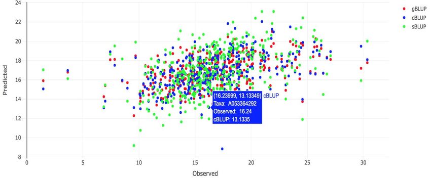
GAPIT User Manual

Disclaimer: While extensive testing has been performed by the Zhiwu Zhang Lab at (2014 to present) at
Washington State University and Edward Buckler Lab (2012-2014) at Cornell University, respectively.
Results are, in general, reliable, correct or appropriate. However, results are not guaranteed for any
specific set of data. We strongly recommend that users validate GAPIT results with other software
packages, such as SAS and TASSEL.

Support documents: Extensive support documents, including this user manual, source code,
demonstration scripts, data, and results, are available at GAPIT website hosted by Zhiwu Zhang
Laboratory: http://zzlab.net/GAPIT

Questions and comments: To benefit GAPIT community, questions and comments should be addressed
to GAPIT forum: https://groups.google.com/forum/#!forum/gapit-forum. The GAPIT team members will
periodically go through these questions and comments and address them accordingly. For countries with
restriction on Google, such as China, questions and comments are welcome to Jiabo Wang by email:
wangjiaboyifeng@163.com.

Citation: Multiple statistical methods are implemented in GAPIT version 1, 2 and 3. Citations of GAPIT
vary depending on methods and versions used in the analysis:

Method                     Method paper                           GAPIT Implimentation
Compression MLM (CMLM)     Zhang et al, 2010, Nature Genetics1    Version 1 by Lipka et al, 2012, Bioinformatics2
gBLUP                      Zhang et al, 2007, J. Anim. Science3   Version 1 by Lipka et al, 2012, Bioinformatics2
Enriched CMLM              Li et al, 2014, BMC Biology4           Version 2 by Tang et al, 2016, The Plant Genome5
SUPER                      Wang et al, 2014, PLoS One6            Version 2 by Tang et al, 2016, The Plant Genome5
MLMM                       Segura et al, 2012, Nature Genetics7   Version 3 by Jiabo Wang and Zhang, 2021, GPB8
FarmCPU                    Liu et al, 2016, PloS Genetics9        Version 3 by Jiabo Wang and Zhang, 2021, GPB8
cBLUP and sBLUP            Wang et al, 2019, Heredity10           Version 3 by Jiabo Wang and Zhang, 2021, GPB8
BLINK                      Huang et al, 2019, GigaScience11       Version 3 by Jiabo Wang and Zhang, 2021, GPB8

Note: These references are listed in section of Reference.

   The GAPIT project is partially supported by USDA, DOE, NSF, the Agricultural Research Center at
                  Washington State University, and Washington Grain Commission

                                                        2
GAPIT User Manual

                                                                  Table of Contents

1     INTRODUCTION .......................................................................................................................................... 6

1.1     WHY GAPIT? ......................................................................................................................................... 6
1.2     GETTING STARTED ................................................................................................................................. 7
1.3     HOW TO USE THE GAPIT USER MANUAL? ............................................................................................... 7

2     INPUT DATA ........................................................................................................................................... 8

2.1 PHENOTYPIC DATA ................................................................................................................................. 8
2.2 GENOTYPIC DATA ................................................................................................................................... 9
2.2.1 HAPMAP FORMAT .................................................................................................................................................9
2.2.2 NUMERIC FORMAT ..............................................................................................................................................10
2.3 KINSHIP ................................................................................................................................................ 11
2.4 COVARIATE VARIABLES ........................................................................................................................ 11
2.5 IMPORT GENOTYPE BY FILE NAMES ..................................................................................................... 12

3     ANALYSIS ................................................................................................................................................. 13

3.1     MIXED LINEAR MODEL (MLM) ............................................................................................................ 15
3.2     COMPRESSED MLM (CMLM) .............................................................................................................. 16
3.3     GENERAL LINEAR MODEL (GLM) ........................................................................................................ 16
3.4     P3D/EMMAX ....................................................................................................................................... 17
3.5     SUPER ................................................................................................................................................... 17
3.6     MULTIPLE LOCUS MIXED LINEAR MODEL (MLMM)............................................................................ 17
3.7     FARMCPU ............................................................................................................................................ 17
3.8     BLINK ................................................................................................................................................. 18
3.9     GENOMIC BLUP ................................................................................................................................... 18
3.10     COMPRESSED GBLUP ............................................................................................................................... 19
3.11     SUPER GBLUP ....................................................................................................................................... 19

4     OUTPUT RESULTS ............................................................................................................................... 20

4.1 PHENOTYPE DIAGNOSIS ........................................................................................................................... 20
4.2 MARKER DENSITY ................................................................................................................................... 20
4.3 LINKAGE DISEQUILIBRIUM DECAY .......................................................................................................... 21
4.4 HETEROZYGOSIS ..................................................................................................................................... 22
4.5 PRINCIPAL COMPONENT (PC) PLOT ........................................................................................................ 22
4.6 KINSHIP PLOT.......................................................................................................................................... 23
4.7 NEIGHBOR-JOINING (NJ)-TREE ................................................................................................................ 25
4.8 QQ-PLOT................................................................................................................................................. 25
4.9 MANHATTAN PLOT .................................................................................................................................. 27
4.10 ASSOCIATION TABLE .............................................................................................................................. 28
4.11 ALLELIC EFFECTS TABLE ...................................................................................................................... 28
4.12 COMPRESSION PROFILE ........................................................................................................................ 28
4.13 THE OPTIMUM COMPRESSION ............................................................................................................... 31

                                                                                  3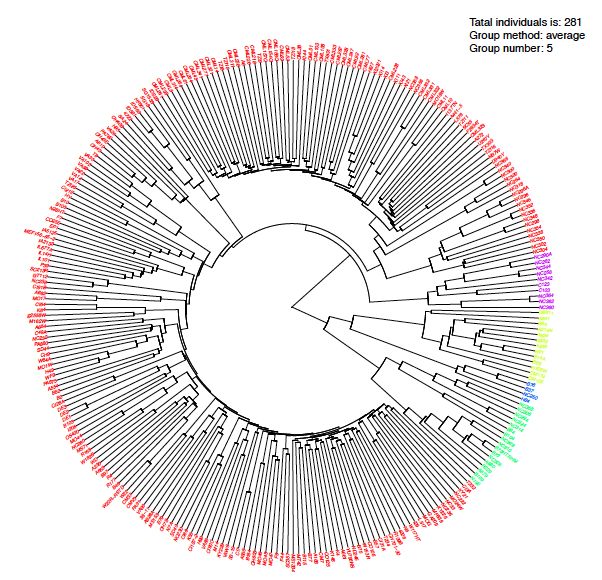
GAPIT User Manual

4.14 MODEL SELECTION RESULTS ................................................................................................................ 31
4.15 MULTIPLE TRAITS OR METHODS............................................................................................................. 32
4.16 GENOMIC PREDICTION .......................................................................................................................... 32
4.17 DISTRIBUTION OF BLUPS AND THEIR PEV. ........................................................................................... 34
4.18 INTERACTIVE GWAS PLOT .................................................................................................................... 35

5     TUTORIALS ............................................................................................................................................... 36

5.1     A BASIC SCENARIO ..................................................................................................................................... 36
5.2     ENHANCED COMPRESSION ........................................................................................................................... 36
5.3     USER-INPUTTED KINSHIP MATRIX AND COVARIATES........................................................................................... 37
5.4     MULTIPLE GENOTYPE FILES .......................................................................................................................... 37
5.5     NUMERIC GENOTYPE FORMAT ...................................................................................................................... 38
5.6     NUMERIC GENOTYPE FORMAT IN MULTIPLE FILES.............................................................................................. 38
5.7     FRACTIONAL SNPS FOR KINSHIP AND PCS ....................................................................................................... 39
5.8     MEMORY SAVING ...................................................................................................................................... 39
5.9     MODEL SELECTION ..................................................................................................................................... 40
5.10     SUPER ................................................................................................................................................. 40
5.11     MLMM ................................................................................................................................................ 40
5.12     FARM-CPU ............................................................................................................................................ 41
5.13     BLINK.................................................................................................................................................... 41
5.14     MULTIPLE MODEL .................................................................................................................................... 41
5.15     GBLUP ................................................................................................................................................. 42
5.16     CBLUP .................................................................................................................................................. 42
5.17     SBLUP .................................................................................................................................................. 42

6     PROTOTYPE.............................................................................................................................................. 43

6.1     PREPARATION ........................................................................................................................................... 43
6.2     GALLERY OF GAPIT GRAPHIC OUTPUT............................................................................................................ 43
6.3     GALLERY OF GAPIT FILE OUTPUT .................................................................................................................. 49
6.4     CROSS VALIDATION WITH REPLACEMENT.......................................................................................................... 49
6.5     CROSS VALIDATION WITHOUT REPLACEMENT .................................................................................................... 51
6.6     CONVERT HAPMAP FORMAT TO NUMERICAL .................................................................................................... 52
6.7     COMPILE SNPS FROM MULTIPLE GAPIT ANALYSES INTO ONE SET OF RESULTS ........................................................... 52
6.8     GENOMIC PREDICTION ................................................................................................................................ 54

7     APPENDIX ............................................................................................................................................. 55

7.1     TUTORIAL DATA SETS.................................................................................................................................. 55
7.2     TYPICAL WAYS OF READING DATA .................................................................................................................. 56
7.3     GAPIT OUTPUT FILES.................................................................................................................................. 57
7.4     FREQUENTLY ASKED QUESTIONS ................................................................................................................... 58
1.     HOW TO CITE GAPIT? ..........................................................................................................................................58
2.     HOW TO DETAIL THE ANALYSIS MODEL? .............................................................................................................58
3.     HOW MANY PCS TO INCLUDE? .............................................................................................................................58
4.     WHAT DO I DO IF I GET FRUSTRATED? .................................................................................................................58
5.     WHY GAPIT HAS DIFFERENT RESULTS FROM OTHER SOFTWARE? ......................................................................58

                                                                                  4
GAPIT User Manual

6.  THERE ARE MANY METHODS IMPLEMENTED IN GAPIT, WHICH ONE SHOULD I USE? .........................................58
7.  IS IT FEASIBLE I COMPARE DIFFERENT MODELS BY MYSELF? ..............................................................................59
8.  HOW DO I REPORT AN ERROR? .............................................................................................................................59
9.  WHAT SHOULD I DO WITH “ERROR IN FILE (FILE, "RT") : CANNOT OPEN THE CONNECTION”? ............................59
10.  WHAT SHOULD I DO WITH “ERROR IN GAPIT (... : UNUSED ARGUMENT(S) ...”? ...............................................59
11.  HOW DEAL WITH “ERROR IN SOLVE.DEFAULT(CROSSPROD(X, X)) : SYSTEM IS COMPUTATIONALLY
SINGULAR”? .................................................................................................................................................................59
12. HOW TO FIX THE ERROR OF USING COVARIATES FROM STRUCTURE AS FIXED EFFECTS? ..............................59
13. SHOULD I REMOVE SNPS WITH MAF BELOW 5%? ............................................................................................59
14. MY TRAIT WAS MEASURED IN MULTIPLE ENVIRONMENTS, HOW DO I USE THEM SIMULTANEOUSLY? ..............59
15. IS IT OK TO ANALYZE BINARY TRAITS (CASE-CONTROL) WITH GAPIT? ...........................................................59
16. WILL NORMALITY TRANSFORMATION HELP? .....................................................................................................59
17. SHOULD I USE PCS OR Q MATRIX? .....................................................................................................................59
7.5 GAPIT BIOGRAPHY .................................................................................................................................... 60
REFERENCES ............................................................................................................................................. 61

                                                                                      5
GAPIT User Manual

1 INTRODUCTION
   1.1 Why GAPIT?
GAPIT implemented a series of methods for Genome Wide Association (GWAS) and Genomic Selection
(GS). The software and related methods received thousands of citations:
Category Publication           Description                                       Year Citations*
Software GAPIT version 1 Implemented GLM, MLM, CMLM and gBLUP                    2012    1264
            GAPIT version 2 Implemented ECMLM and SUPER                          2016    207
            GAPIT version 3 Implemented MLM, FarmCPU, BLINK,                     2021     13
                               cBLUP and sBLUP
GWAS        MLM                Known as QK model to control both population      2005   3,238
                               (Q matrix) structure and kinship (K).
            Compressed         Individual is compressed into groups to reduce    2010   1,533
            MLM                confounding between kinship and testing
                               markers.
            SUPER              Derived kinship from associated markers           2014    153
                               (QTNs) instead of all markers and use QTNs
                               that are complementary to testing markers.
            Enriched           Optimization of group kinship                     2014     72
            compressed
            MLM
            MLMM               Step wise regression to include associated        2012    619
                               markers in MLM
            FarmCPU            Select associated markers as cofactor to control  2016    469
                               false positives using likelihood in MLM to
                               avoid overfitting and test markers without
                               kinship to eliminate confounding between
                               kinship and testing markers in iterative fashion.
            BLINK              Use GLM and Bayesian Information Content          2019     62
                               using batch stepwise regression
GS          gBLUP              Use RFLP markers to derive kinship among          1994    317
                               maize lines to estimate breeding values
            Marker based       Add second path to use kinship derived from       2006     50
            MTDFREML           markers
            Efficient kinship Define kinship as marker matrix multiplied by      2008   3,614
                               its transpose.
            sBLUP              Derive kinship from QTNs from SUPER               2019     29
                               method to estimate breeding values. The
                               method has higher prediction accuracy than
                               gBLUP for traits controlled with less number of
                               genes.
            cBLUP              Estimate individuals’ breeding values by the      2019     29
                               breeding values of their corresponding groups.
                               The method has higher prediction accuracy than
                               gBLUP for traits with low heritability.
*Google Scholar by September 5, 2021,

                                               6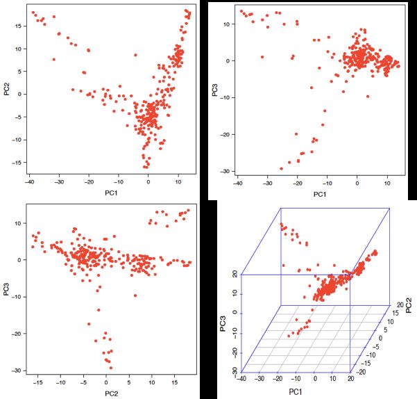
GAPIT User Manual

   In addition to the multiple available methods, GAPIT is user friendly and produces comprehensive
reports to interpret data and results in publication ready formats. For examples, GAPIT accept both
numeric and hapmap genotype formats. The individuals in the phenotype files do not have to be in the
same order as genotype files, or even can be partially different. GAPIT produces the distribution of
marker density and decay of linkage equilibrium to inform user if the markers are dense enough. When
multiple GWAS methods are selected, GAPIT produces the corresponding Manhattan plots with
overlapped associated markers highlighted as illustrated on the right for the GAPIT demo data from
maize. The results show that GLM method identified association signals above the Bonferroni threshold
(dash red lines). However, the association signals are inflated across the genome (the red dots on the QQ
plots). BLINK method identified two associated markers, including the marker close to a flowering time
gene, VGT1 on chromosome 8. The QQ plot suggests that 99% of the markers have p values under
expectation indicated by the solid red line.

   1.2 Getting Started
GAPIT is a package that is run in the R software environment, which can be freely downloaded from
http://www.r-project.org or http://www.rstudio.com. There are two sources to install GAPIT package.
Zhiwu Zhang Lab website:
 source("http://zzlab.net/GAPIT/GAPIT.library.R")
 source("http://zzlab.net/GAPIT/gapit_functions.txt")

GitHub:
 install.packages("devtools")
 devtools::install_github("jiabowang/GAPIT3",force=TRUE)
 library(GAPIT3)

The easiest way of using GAPIT is to COPY/PASTE GAPIT tutorial script. Here is an example using five
methods using the data from Zhiwu Zhang Lab website.
 #Import data from Zhiwu Zhang Lab
 myY
GAPIT User Manual

2 Input Data
There are size types of input data: phenotype (Y), genotype in hapmap format (G), genotype data in
numerical format (GD), genotype map (GM), kinship (K), and covariate variables (CV), see Table 2.1.
Phenotypic data must be provided and the rest are optional, including genotype data, map, kinship, and
covariate. Kinship can be provided by users or be generated from genotype data, or even omitted by suing
BLINK method. Genotypic data may not be needed for genomic prediction if the kinship matrix is
provided by the user. Covariate variables (fixed effects), such as population structure represented by the Q
matrix (subpopulation proportion) or principal components (PCs), are optional. GAPIT provides the
option to calculate PCs from the genotypic data. All input files should be saved as a “Tab” delimited text
file.

Notice: It is important that each taxa name is spelled, punctuated, and capitalized (R is case sensitive) the
same way in each of the input data sets. If this is not done, they will be excluded from the analysis.
Additionally, the taxa names must not be numeric.

Table 2.1 Gallery of GAPIT input data

 Parameter       Default   Options       Description
 Y               NULL      User          Phenotype
 KI              NULL      User          Kinship Matrix
 CV              NULL      User          Covariate Variables
 G               NULL      User          Genotype Data in Hapmap Format
 GD              NULL      User          Genotype Data in Numeric Format
 GM              NULL      User          Genotype Map for Numeric Format
 file.Ext.G      NULL      User          File Extension for Genotype in Hapmap Format
 file.Ext.GD     NULL      User          File Extension for Genotype Data in Numeric Format
 file.Ext.GM     NULL      User          File Extension for Genotype Map for Numeric Format
 file.fragment   NULL      User          The Fragment Size to Read Each Time within a File
 file.G          NULL      User          The Common Name of File for Genotype in Hapmap Format
 file.GD         NULL      User          The Common Name of File for Genotype Map for Numeric Format
 file.GM         NULL      User          The Common Name of File for Genotype Data in Numeric Format
 file.path       NULL      User          Path for Genotype Files
 file.from       0         >0            The First Genotype Files Named Sequentially
 file.to         0         >0            The Last Genotype Files Named Sequentially
Notice: The inputs in italic are supported by GAPIT version 1 and 2 (before 2017) only.

   2.1 Phenotypic Data
The user has the option of performing GWAS on multiple phenotypes in GAPIT. This is achieved by
including all phenotypes in the text file of phenotypic data. Taxa names should be in the first column of
the phenotypic data file and the remaining columns should contain the observed phenotype from each
individual. Missing data should be indicated by either “NaN” or “NA”. The first ten observations in the
tutorial data (mdp_traits.txt) are displayed as follows:

                                                     8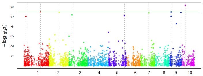
GAPIT User Manual

The file is “Tab” delimited. The first row consists of column labels (i.e., headers). The column labels
indicate the phenotype name, which is used for the remainder of the analysis.

The phenotype file can be input to R by typing command line:

 myY
GAPIT User Manual

Although all of the first 11 columns are required, GAPIT uses only 3 of these: the “rs” column, which is
the SNP name (e.g. “PZB00859.1”); the “chrom” column, which is the SNP’s chromosome; and the “pos”,
which is the SNP’s base pair (bp) position. It is sufficient to fill in the requested information in the
remaining eight columns with “NA”s. To be consistent with HapMap naming conventions, missing
genotypic data are indicated by either “NN” (double bit) or “N” (single bit).

For genotypic data in HapMap format, GAPIT accepts genotypes in either double bit or in the standard
IUPAC code (single bit) as following:

Genotype AA CC GG TT AG CT CG AT GT AC
Code      A C G T R Y S W K M

By default, the HapMap numericalization is performed so that the sign of the allelic effect estimate (in the
GAPIT output) is with respect to the nucleotide that is second in alphabetical order. For example, if the
nucleotides at a SNP are “A” and “T”, then a positive allelic effect indicates that “T” is favorable.
Selecting “Major.allele.zero = TRUE” in the GAPIT() function will result in the sign of the allelic effect
estimate being with respect to the minor allele. In this scenario, a positive allelic effect estimate will
indicate that the minor allele is favorable.

2.2.2 Numeric format
GAPIT also accepts the numeric format used by EMMA. Columns are used for SNPs and rows are used
for taxa. This format is problematic in Excel because the number of SNPs used in a typical analysis
exceeds the Excel column limit. Additionally, this format does not contain the chromosome and position
(physical or genetic) of the SNPs. Therefore, two separate files must be provided to GAPIT. One file
contains the numeric genotypic data (called the “GD” file), and the other contains the position of each
SNP along the genome (called the “GM” file). Note: The SNPs in the “GD” and “GM” files NEED to be
in the same order.

Homozygotes are denoted by “0” and “2” and heterozygotes are denoted by “1” in the “GD” file. Any
numeric value between “0” and “2” can represent imputed SNP genotypes. The first row is a header file
with SNP names, and the first column is the taxa name.

Example file (mdp_numeric.txt from tutorial data set):

                     taxa            PZB00859.1 PZA01271.1 PZA03613.2 PZA03613.1
                     33-16                    2          0          0          2
                     38-11                    2          2          0          2
                     4226                     2          0          0          2
                     4722                     2          2          0          2
                     A188                     0          0          0          2
                       …

This file is read into R by typing the following command line:

 myGD
GAPIT User Manual
The “GM” file contains the name and location of each SNP. The first column is the SNP id, the second
column is the chromosome, and the third column is the base pair position. As seen in the example, the
first row is a header file.
Example file (mdp_SNP_information.txt from tutorial data set):
Name Chromosome Position
PZB00859.1 1 157104
PZA01271.1 1 1947984
PZA03613.2 1 2914066
PZA03613.1 1 2914171
PZA03614.2 1 2915078
…
This file is read into R by typing the following command line:
myGMGAPIT User Manual Example file (mdp_population_structure.txt from tutorial data set): This file is read into R by typing the following command line: myCV
GAPIT User Manual

3 Analysis
GAPIT implemented a series of methods for GWAS and genomic selection toward high statistical power,
high prediction accuracy, and high computing speed, see Figure 3.1. The methods include General Linear
Model (GLM), Mixed Linear Model (MLM), Compressed MLM (CMLM), Enriched CMLM
(ECMLM), Settlement of MLM Under Progressively Exclusive Relationship (SUPER), Fixed and
random model Circulating Probability Unification (FarmCPU), and Bayesian-information and Linkage-
disequilibrium Iteratively Nested Keyway (BLINK).

Figure 3.1. Methods implemented in GAPIT for GWAS and genomic selection. All the methods support
GWAS, including General Linear Model (GLM), Mixed Linear Model (MLM), Compressed MLM
(CMLM), Enriched CMLM (ECMLM), Settlement of MLM Under Progressively Exclusive
Relationship (SUPER), Fixed and random model Circulating Probability Unification (FarmCPU), and
Bayesian-information and Linkage-disequilibrium Iteratively Nested Keyway (BLINK). Some of these
methods support genomic selection, including MLM, CMLM, ECMLM, SUPER, and FarmCPU. The
remaining (GLM and BLINK) can be used for breeding through marker assisted selection (MAS).

                                                 13
GAPIT User Manual
The similarity and difference among
these methods are summarized in the
figure on the right. The most simplest
model is to directly detect the
association between a phenotype (y) and
markers (Si) one at a time, where i=1 to
m, and m is number of markers. When a
cofactor, such as population structure (Q)
is introduced through a general linear
model (GLM), the cofactor may not
only account residuals (e) partially, but
also adjust some effect that does not
belong to the testing markers and
consequently reduce false positives. The
mixed linear model (MLM) applies the
same principle by adding individuals’
genetic effects as random cofactor
effects with variance structure defined
by the kinship (K) among individuals. In
both Q or Q+K models, Q and K stay
the same. There are no cofactors that are
adjusted by the marker tests.
The situation was changed by the
multiple loci mixed model (MLMM).
Through marker association tests, the
associated markers are fitted as the
cofactors for marker test. The cofactors
are adjusted through forward and
backward stepwise regression of mixed
model. However, both Q and K remain
unchanged.
In SUPER method, K is derived from the associated and markers and is adjected accordingly by the
marker tests. As the K is derived from a smaller number of markers than the K in MLM and MLMM that
are derived from all the markers, the confounding between K and some of markers become more severe.
SUPER eliminate the confounding by using the complementary kinship derived from associated markers
except the ones that are in strong linkage disequilibrium (LD) with the testing markers under a user
defined threshold.
To eliminate the ambiguous of determining associated markers are in LD with a testing marker, FarmCPU
completely remove the confounding from kinship by using a fixed effect model without a kinship derived
either from all markers, or associated markers. Instead the kinship derived from the associated markers is
used to select the associated markers using maximum likelihood method. This process overcome the
model overfitting problems of stepwise regression. FarmCPU uses both fixed effect model and the
random effect model iteratively.
The random effect model in FarmCPU to select associated markers using maximum likelihood method
remains a high computing cost for large number of individuals. BLINK approximate the maximum
14GAPIT User Manual
likelihood using Bayesian Information Content (BIC) in a fixed effect model to eliminate the
computational burden. BLINK also eliminate the assumption that causal genes are evenly distributed
across genome required by SUPER and FarmCPU methods. Consequently, BLINK is not only superior to
FarmCPU for computing speed, but also for high statistical power and less false positives.
Among these methods, researches demonstrated that method on higher stars has higher statistical power
for GWAS than the one on lower stars. These differences disappear in some cases suggesting interactions
between the methods and other factors, including populations, environments, and traits. For examples, all
methods work well for cases with extreme high heritability and major genes, or do not work for the
opposite situation. In all conditions, the order of statistical powers stay the same among all the methods.
The inversion of the order has not been found.
However, the interactions have been found for genomic selection. The genomic selection based on
SUPER, named SUPER BLUP, has higher prediction accuracy than the genomic selection based on MLM
known as genomic BLUP (gBLUP) for traits controlled with a smaller number of genes. The prediction
accuracies are reversed for traits controlled by a large number of genes. The genomic selection based on
CMLM, named Compressed BLUP, has higher accuracy for traits with low heritability than gBLUP.
Table 3.1. GAPIT input parameters.
Parameter Default Options Description
GLM, MLM, CMLM, SUPER,
model Blink Choose model to conduct GWAS
MLMM, FarmCPU, and Blink
kinship.algorithm VanRaden Zhang, Loiselle and EMMA Algorithm to Derive Kinship from Genotype
complete, ward, single,
kinship.cluster average Clustering algorithm to group individuals based on their kinship
mcquitty, median, and centroid
kinship.group Mean Max, Min, and Median Method to derive kinship among groups
group.from 1 User The starting number of groups of iteration
The ending number of groups of iteration, if larger than number of
group.to 1000000 User
individuals (n), n is used.
group.by 10 User Iteration interval for number of groups
LD.chromosome NULL User Chromosome for LD analysis
LD.location NULL User Location (center) of SNPs for LD analysis
LD.range NULL User Range around the Central Location of SNPs for LD Analysis
PCA.total 0 >0 Total Number of PCs as Covariates
PCA.scaling None Scaled, Centered.and.scaled Scale And/Or Center And Scale The SNPs Before Conducting PCA
SNP.FDR 1 >0 and 0 and 0 andGAPIT User Manual
STRUCTURE12 or conducting a principal component analysis13), the “Q+K” approach improves
statistical power compared to “Q” only14. An MLM can be described using Henderson’s matrix notation
as follows:
Y = Xβ + Zu + e, (1)
where Y is the vector of observed phenotypes; β is an unknown vector containing fixed effects, including
the genetic marker, population structure (Q), and the intercept; u is an unknown vector of random additive
genetic effects from multiple background QTL for individuals/lines; X and Z are the known design
matrices; and e is the unobserved vector of residuals. The u and e vectors are assumed to be normally
distributed with a null mean and a variance of:
u G 0
Var =
e 0 R (2)
where G = σ2aK with σ2a as the additive genetic variance and K as the kinship matrix. Homogeneous
variance is assumed for the residual effect; i.e., R= σ2eI, where σ2e is the residual variance. The proportion
of the total variance explained by the genetic variance is defined as heritability (h2).
σ a2
h2 =
σ a2 + σ e2 , (3)
3.2 Compressed MLM (CMLM)
As kinship is derived from all the markers, incorporating with the kinship for testing markers in a MLM
causes the confounding between the testing markers and the individuals’ genetic effects with variance
structure defined by the kinship. To reduce the confounding, individuals are replaced by their
corresponding groups in the compressed MLM developed by Zhang et al in 2010 15. Cluster analysis is
used to assign similar individuals into groups. The elements of the kinship matrix are used as similarity
measures in the clustering analysis. Various linkage criteria (e.g., unweighted pair group method with
arithmetic mean, UPGMA) can be used to group the lines together. The number of groups is specified by
the user. Once the lines are assigned into groups, summary statistics of the kinship between and within
groups are used as the elements of a reduced kinship matrix. This procedure is used to create a reduced
kinship matrix for each compression level.
A series of mixed models are fitted to determine the optimal compression level. The value of the log
likelihood function is obtained for each model, and the optimal compression level is defined as the one
whose fitted mixed model yields the largest log likelihood function value. There are three parameters to
determine the range and interval of groups for examination: group.from, group.to and group.by. Their
defaults are 0, n and 10, where n is the total number of individuals.
3.3 General Linear Model (GLM)
Regular MLM16 is an extreme case of CMLM where each individual is considered as a group. It can be
simply performed by setting the number of groups equal to the total number of individuals, e.g.
group.from = n and group.to = n, where n is total number of individuals shared in both the genotype and
phenotype files. Similarly, general linear model (GLM) is another extreme case of CMLM where all
individuals are considered as one group. It can be simply performed by setting the number of groups equal
16GAPIT User Manual
to one, i.e. group.from = 1 and group.to = 1. GLM is the working model in PLINK17, a primary software
for studies in human genetics.
3.4 P3D/EMMAx
In addition to implementing compression, GAPIT uses EMMAx/P3D1,18 to reduce computing time for
MLM, CMLM, ECMLM, and SUPER. If specified, the additive genetic (σ2a) and residual (σ2e) variance
components will be estimated prior to conducting GWAS. These estimates are then used for each SNP
where a mixed model is fitted.
3.5 SUPER
SUPER is an advanced version of FaST-Select, developed Wang et al. in 2016. The major difference
between SUPER and FaST-Select is that SUPER uses bin approach to select associated markers. The
entire genome is divided into equal sized bins and each bin is represented by the most significant marker
on the bin. The bin size and number of bins selected are optimized using maximum likelihood method in a
random model with the kinship derived from the selected bins. Consequently, the confounding between
the kinship and some of markers become more severe than the kinship derived from all markers. SUPER
eliminate the confounding by using the complementary kinship derived from associated markers except
the ones that are in strong linkage disequilibrium (LD) with the testing markers under a user defined
threshold. Both simulation and real data demonstrated that SUPER had higher statistical power than
regular MLM.
To run SUPER in GAPIT, simply specify model= "SUPER".
3.6 Multiple Locus Mixed Linear Model (MLMM)
GAPIT implemented a Multiple Loci Mixed Linear Model (MLMM) which use forward-backward
stepwise linear mixed-model regression to include associated markers as covariates.
To run MLMM in GAPIT, simply specify model= "MLMM".
3.7 FarmCPU
To solve the problem of false positive control and confounding between testing markers and cofactors
simultaneously, an iterative method, named Fixed and random model Circulating Probability Unification
(FarmCPU), was developed in 20169. The associated markers detected from the iterations are fitted as
the cofactors to control false positives for testing the rest markers in a fixed effect model. To avoid the
over model fitting problem in stepwise regression, a random effect model is used to select the associated
markers using maximum likelihood method9.
In the cycle of fixed effect model of iterations, markers are tested against the associated markers, not the
confounded kinship used by MLM, CMLM, ECMLM, SUPER, and MLMM. In the cycle of random
effect model of iterations, markers are selected among a small number of associated markers using
maximum likelihood method to avoid the over model fitting problem in stepwise regression used by
MLMM, which select marker among all available markers. Consequently, FarmCPU exhibits higher
statistical power than MLMM9. As FarmCPU tests markers in a fixed effect model, it is computational
efficient than the methods that test markers in random effect model, such as MLM, CMLM, ECMLM,
SUPER, and MLMM9.
To run FarmCPU in GAPIT, simply specify model= "FarmCPU".
17GAPIT User Manual
3.8 BLINK
BLINK method was designed to have both high statistical power and computational efficiency 11. It was
inspired by FarmCPU method with two major changes to achieve the objectives. One is to eliminate the
assumption that causal genes are evenly distributed across genome that required by FarmCPU. As the
assumption cause either inclusion of non causal genes, or missing the causal genes that are in the same bin
with another causal genes with stronger signal. BLINK works directly on markers instead of bins.
Markers that are in linkage disequilibrium (LD) with the most significant marker are excluded. For the
second remaining marker, the exclusion is conducted in the same way as the most significant marker, so
on and so forth until no marker can be excluded.
The other change is to use Bayesian Information Content (BIC) of a fixed effect model to approximate the
maximum likelihood of a random effect model to select the associated markers among the markers
remained the exclusion based on LD. As both the models of testing markers and selecting associated
markers as cofactors are fixed effect model, the computation complexity reach the maximum. A dataset
with one million individuals and one million markers can be solved in hours by using BLINK C version.
The BLINK R version can be run as standard alone, or through GAPIT. To run BLINK in GAPIT, simply
specify model= "Blink". The performances of the two versions were documented by the BLINK article on
GigaScience11.
3.9 Genomic BLUP
Genomic prediction is performed with the method based on genomic best linear unbiased prediction,
(gBLUP)3. The method was extended to compressed best linear unbiased prediction (cBLUP) by using the
CMLM approach that was proposed for GWAS1. The genetic potential for a group, which is derived from
the BLUPs of group effects in the compressed mixed model, is used as a prediction for all individuals in
the group.
The groups created from compression belong to either a reference (R) or an inference (I) panel. All groups
in the reference panel have at least one individual with phenotypic data, and all groups in the inference
panel have no individuals with phenotypic data. Genomic prediction for groups in the inference panel is
based on phenotypic ties with corresponding groups in the reference panel.
The group kinship matrix is then partitioned into to R and I groups as follows:
k k RI
k= RR
k II
(4)
k IR ,
where kRR is the variance-covariance matrix for all groups in the reference panel, kRI is the covariance
matrix between the groups in the reference and inference panels, kIR = (kRI)’ is the covariance matrix
between the groups inference and reference panels, and kII is the variance-covariance matrix between the
groups in the inference panels.
Solving of mixed linear model is performed on the reference individuals.
yR =X R + ZR u R + eR , (5)
where all terms are as defined in Equation (1), and the “R” subscript denotes that only individuals in the
reference panel are considered.
The genomic prediction of the inference groups is derived Henderson’s formula (1984) as follows:
u I =K IR K -1RR uR 18GAPIT User Manual
, (6)
where kIR, kRR , and uR are as previously defined, and uI is the predicted genomic values of the
individuals in the inference group.
The reliability of genomic prediction is calculated as follows:
PEV
Reliability=1- (7)
a2
where PEV is the prediction error variance which is the diagonal element in the inverse left-hand side of
the mixed model equation, and a is the genetic variance.
2
3.10 Compressed gBLUP
The compressed MLM substitute individuals with their corresponding groups that were clustered based on
the kinship among individuals. Research demonstrate that the compressed MLM had higher statistical
power for GWAS. Research also demonstrated that compressed MLM also had higher prediction accuracy
than the regular MLM, especially for traits with low heritability. As the regular MLM is an extreme case
of compressed MLM, the compressed MLM has higher, or at least equal prediction accuracy as the
regular MLM. When a compressed MLM is specified in GAPIT, individuals’ breeding values are
predicted by the breeding values of their corresponding groups.
3.11 SUPER gBLUP
The regular MLM uses the kinship derived from all the markers while SUPER uses the kinship derived
from the associated markers. As the associated markers are selected from all the markers using the
maximum likelihood method, the kinship used by SUPER has better likelihood than the kinship used by
the regular MLM. Researches demonstrated that the estimated breeding values from SUPER had higher
prediction accuracy than the estimated breeding values from the regular MLM.
19GAPIT User Manual
4 Output Results
GAPIT produces a series of output files that are saved in two formats. All tabular results are saved as
comma separated value (.csv) files, and all graphs are stored as printable document format (.pdf) files.
This section provides descriptions of these output files.
4.1 Phenotype diagnosis
GAPIT diagnosis phenotype in several ways, including scatter plot, histogram, box plot and accumulative
distribution.
4.2 Marker density
Marker density is critical to establish Linkage Disequilibrium (LD) between markers and causal mutations.
Comparison between the marker density and the LD decade over distance provides the indication if
markers are dense enough to have good coverage of LD.
20GAPIT User Manual
Figure 4.2.1 Frequency and accumulative frequency of marker density. Distribution of marker density is
displayed as a histogram and an accumulative distribution.
4.3 Linkage Disequilibrium Decay
Linkage disequilibrium are measured as R square for pair wise markers and plotted against their distance.
The moving average of adjacent markers were calculated by using a sliding windows with ten markers.
21GAPIT User Manual
Figure 4.3.1 Linkage disequilibrium (LD) decay over distance. LDs were calculated on sliding windows
with 100 adjacent genetic markers. Each dot represents a pair of distances between two markers on the
window and their squared correlation coefficient. The red line is the moving average of the 10 adjacent
markers.
4.4 Heterozygosis
The frequency of heterozygous were calculated for both individuals and markers. High level of
heterozygosis indicated low quality. For example, over 50% of heterozygosis on inbred lines for some of
markers suggested they problematic (see bottom right).
4.5 Principal Component (PC) plot
For each PC included in the GWAS and GPS models, the observed PC values are plotted.
22GAPIT User Manual
Figure 4.5.1 Pair-wise plots and 3D plots of principal component (PC).
4.6 Kinship plot
The kinship matrix used in GWAS and GPS is visualized through a heat map. To reduce computational
burden, this graph is not made when the sample size exceeds 1,000.
23GAPIT User Manual
Figure 4.6.1 Kinship plot. A heat map of the kinship matrix is created to indicate the relationship between
individuals.
24GAPIT User Manual
4.7 Neighbor-Joining (NJ)-tree
Following the compress group, we classify individuals to explain population structure. We also
can plot group PCA plot with previous group.
Figure 4.7.1 Neighbor-Joining (NJ)-tree The whole population was divided into 5 clusters with each
colors.
4.8 QQ-plot
The quantile-quantile (QQ) –plot is a useful tool for assessing how well the model used in GWAS
accounts for population structure and familial relatedness. In this plot, the negative logarithms of the P-
values from the models fitted in GWAS are plotted against their expected value under the null hypothesis
of no association with the trait. Because most of the SNPs tested are probably not associated with the trait,
the majority of the points in the QQ-plot should lie on the diagonal line. Deviations from this line suggest
the presence of spurious associations due to population structure and familial relatedness, and that the
GWAS model does not sufficiently account for these spurious associations. It is expected that the SNPs
on the upper right section of the graph deviate from the diagonal. These SNPs are most likely associated
with the trait under study. By default, the QQ-plots in GAPIT show only a subset of the larger P-values
(i.e., less significant P-values) to reduce the file size of the graph.
25GAPIT User Manual
Figure 4.8.1 Quantile-quantile (QQ) –plot of P-values. The Y-axis is the observed negative base 10
logarithm of the P-values, and the X-axis is the expected observed negative base 10 logarithm of the P-
values under the assumption that the P-values follow a uniform[0,1] distribution. The dotted lines show
the 95% confidence interval for the QQ-plot under the null hypothesis of no association between the SNP
and the trait.
26GAPIT User Manual
4.9 Manhattan Plot
The Manhattan plot is a scatter plot that summarizes GWAS results. The X-axis is the genomic position
of each SNP, and the Y-axis is the negative logarithm of the P-value obtained from the GWAS model
(specifically from the F-test for testing H0: No association between the SNP and trait). Large peaks in the
Manhattan plot (i.e., “skyscrapers”) suggest that the surrounding genomic region has a strong association
with the trait. GAPIT produces one Manhattan plot for the entire genome (Figure 3.4) and individual
Manhattan plots for each chromosome.
Figure 4.9.1 Manhattan plot. The X-axis is the genomic position of the SNPs in the genome, and the Y-
axis is the negative log base 10 of the P-values. Each chromosome is colored differently. SNPs with
stronger associations with the trait will have a larger Y-coordinate value.
27GAPIT User Manual
4.10 Association Table
The GWAS result table provides a detailed summary of appropriate GWAS results. The rows display the
results for each SNP above the user-specified minor allele frequency threshold. The SNPs sorted by their
P values (from smallest to largest).
Table 4.10.1 GWAS results for all SNPs that were analyzed.
This table provides the SNP id, chromosome, bp position, P-value, minor allele frequency (maf), sample
size (nobs), R2 of the model without the SNP, R2 of the model with the SNP, and adjusted P-value
following a false discovery rate (FDR)-controlling procedure19.
4.11 Allelic Effects Table
A separate table showing allelic effect estimates is also included in the suite of GAPIT output files. The
SNPs, presented in the rows, are sorted by their position in the genome.
Table 4.11.1 Information of associated SNPs.
This table provides the SNP id, chromosome, bp position, and the allelic effect estimate of each SNP
analyzed.
4.12 Compression Profile
There are seven algorithms available to cluster individuals into groups for the compressed mixed linear
model. There are also four summary statistics available for calculating the group kinship matrix. When
only one group number (i.e., one dimension for the group kinship matrix) is specified, a column chart is
created to illustrate the compression profile for 2*log likelihood function (the smaller the better), genetic
variance, residual variance and the estimated heritability.
28GAPIT User Manual
Figure 4.12.1. Compression profile with single group. The X-axis on all graphs display the summary
statistic method used to obtain the group kinship matrix. The rectangles with different colors indicate the
clustering algorithm used to group individuals.
Note: This graph is not created when multiple groups are specified.
29GAPIT User Manual
When a range of groups (i.e., a range of dimensions for the group kinship matrix) is specified, a different
series of graphs are created. In this situation, the X-axis displays the group number. Lines with different
style and colors are used to present the combinations between clustering algorithm and the algorithm to
calculate kinship among groups.
Figure 4.12.2. Compression profile over multiple groups. The X-axis on each graph is the number of
groups considered, and the Y-axes on the graphs are the -2*log likelihood function, the estimated genetic
variance components, the estimated residual variance component, the estimated total variance, and the
heritability estimate. Each clustering method and group kinship type is represented as a line on each graph.
Notice: This graph is not created when only one group is specified.
30GAPIT User Manual
4.13 The Optimum Compression
Once the optimal compression settings are determined, GAPIT produces a PDF file containing relevant
detailed information. This information includes the optimal algorithm to calculate the group kinship
matrix, the optimal clustering algorithm, the optimal number of groups, -2*log likelihood function and
the estimated heritability.
Figure 4.13.1 The profile for the optimum compression. The optimal method to calculate group kinship is
“Mean”, the optimal clustering method is “average”, the number of groups (ie., the dimension of the
group kinship matrix) is 251, the value of -2*log likelihood function is 1800.11, and the heritability is
41.6%.
4.14 Model Selection Results
By selecting “Model.selection = TRUE”, forward model selection using the Bayesian information
criterion (BIC) will be conducted to determine the optimal number of PCs/Covariates to include for each
phenotype. The results summary (below) for model selection are stored in a .csv file called
“.BIC.Model.Selection.Results”.
Table 4.14.1 Summary for Bayesian information criterion (BIC) model selection results.
31GAPIT User Manual
The number of PCs/Covariates, the BIC value, and the log Likelihood function value are presented. In this
table, the optimal number of PCs to include in the GWAS model is 2.
4.15 Multiple traits or methods
There are several new method integrated in. Furthermore, more than single method or trait result, we
propose a multiple method or traits Manhattan and QQ plots for comparison with methods or traits, this
part is based on MVP library to exhibit. There are two types of Manhattan plots (Orthogon and
Roundness).
Figure 4.15.1 Multiple traits or methods Manhattan and QQ plot. The dash line in the Figure A indicated
the common significant markers were detected by two methods or traits. The solid line in the Figure A
indicated the common significant markers were detected by more than two methods or traits.
4.16 Genomic Prediction
The genomic prediction results are saved in a .csv file.
Table 4.16.1 Genomic Breeding values and prediction error variance.
32GAPIT User Manual
The individual id (taxa), group, RefInf which indicates whether the individual is in the reference group (1)
or not (2), the group ID number, the BLUP, and the PEV of the BLUP.
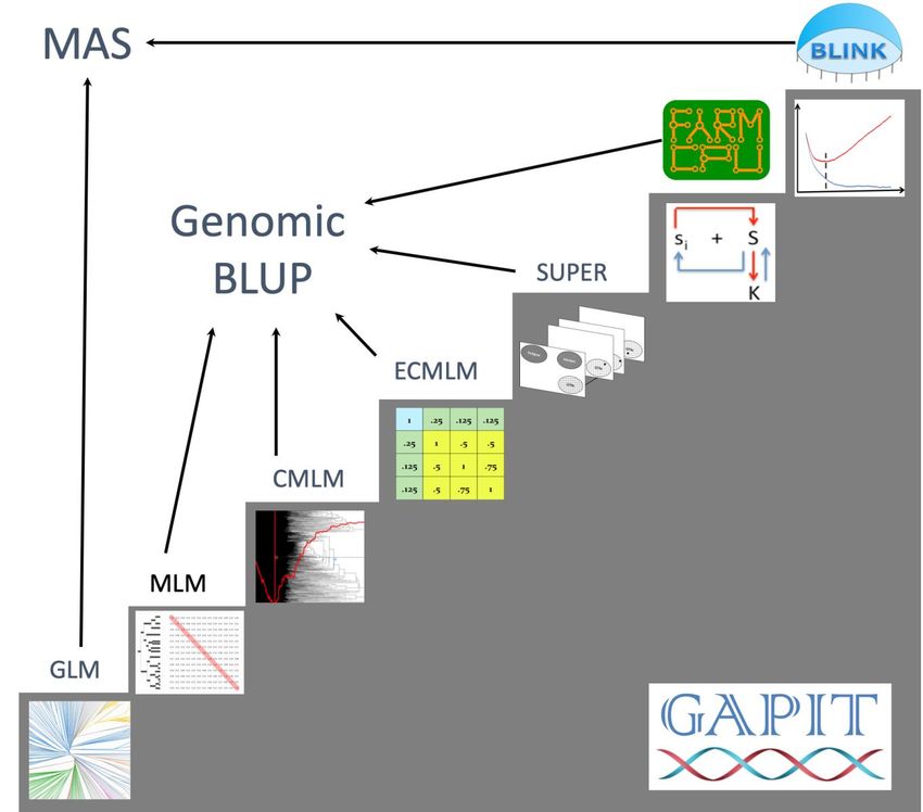
Figure 4.16.1 Interactive GS plot for gBLUP, cBLUP and sBLUP.
33GAPIT User Manual
4.17 Distribution of BLUPs and their PEV.
A graph is provided to show the joint distribution of GBV and PEV. The correlation between them is an
indicator of selection among the sampled individuals 20.
Figure 4.17.1 Joint distribution of genomic breeding value and prediction error variance.
34GAPIT User Manual
4.18 Interactive GWAS plot
A graph is provided to show the Interactive Manhattan and QQ plot with “Inter.Plot=T”. These files are
HTML and supported to act with mouse. The more details of SNP will be showed when the mouse moved
on the point.
Figure 4.18.1 Interactive Manhattan and QQ plot.
35GAPIT User Manual 5 Tutorials The “Getting started” section should be reviewed before running these tutorials, and it is assumed that the GAPIT package and its required libraries have been installed. These tutorials begin with a scenario requiring minimal user input. Subsequent scenarios require a greater amount of user input. Each scenario involves two steps: reading in the data and then running the GAPIT() function. All tutorials are available on the GAPIT home page, which also contains the R source code and results for all the scenarios. The GAPIT maize demonstration data (described at www.panzea.org) are from a maize association panel consisting of 281 diverse lines21. The genotypic data consist of 3,093 SNPs distributed across the maize genome, and are available in HapMap and numeric format. The three phenotypes included are ear height, days to pollination, and ear diameter. The kinship matrix was calculated using the method of Loiselle et al.22 and the fixed effects used to account for population structure were obtained from STRUCTURE 23. Notice: It is important that the correct paths to the directories are specified. Please note that two backward slashes (“\\”) are necessary when specifying these paths. 5.1 A Basic Scenario The user needs to provide two data sets (phenotype and genotype) and one input parameter. This parameter, “PCA.total”, specifies the number of principal components (PCs) to include in the GWAS model. GAPIT will automatically calculate the kinship matrix using the VanRaden method 24, perform GWAS and genomic prediction with the optimum compression level using the default clustering algorithm (average) and group kinship type (Mean). The scenario assumes that the genotype data are saved in a single file in HapMap format. If the working directory contains the tutorial data, the analysis can be performed by typing these command lines: #Step 1: Set data directory and import files myY
You can also read