Bayesian method for causal inference in spatially-correlated multivariate time series - arXiv
←
→
Page content transcription
If your browser does not render page correctly, please read the page content below
Bayesian Analysis (2018)                    00, Number 0, pp. 1–28

                                                  Bayesian method for causal inference in
                                                spatially-correlated multivariate time series
                                                               Bo Ning∗ , Subhashis Ghosal∗ and Jewell Thomas†‡
arXiv:1801.06282v3 [stat.ME] 12 Mar 2018

                                                 Abstract.
                                                     Measuring the causal impact of an advertising campaign on sales is an essential
                                                 task for advertising companies. Challenges arise when companies run advertising
                                                 campaigns in multiple stores which are spatially correlated, and when the sales
                                                 data have a low signal-to-noise ratio which makes the advertising effects hard to
                                                 detect. This paper proposes a solution to address both of these challenges. A novel
                                                 Bayesian method is proposed to detect weaker impacts and a multivariate struc-
                                                 tural time series model is used to capture the spatial correlation between stores
                                                 through placing a G-Wishart prior on the precision matrix. The new method is to
                                                 compare two posterior distributions of a latent variable—one obtained by using
                                                 the observed data from the test stores and the other one obtained by using the
                                                 data from their counterfactual potential outcomes. The counterfactual potential
                                                 outcomes are estimated from the data of synthetic controls, each of which is a
                                                 linear combination of sales figures at many control stores over the causal period.
                                                 Control stores are selected using a revised Expectation-Maximization variable
                                                 selection (EMVS) method. A two-stage algorithm is proposed to estimate the pa-
                                                 rameters of the model. To prevent the prediction intervals from being explosive, a
                                                 stationarity constraint is imposed on the local linear trend of the model through a
                                                 recently proposed prior. The benefit of using this prior is discussed in this paper.
                                                 A detailed simulation study shows the effectiveness of using our proposed method
                                                 to detect weaker causal impact. The new method is applied to measure the causal
                                                 effect of an advertising campaign for a consumer product sold at stores of a large
                                                 national retail chain.
                                                 MSC 2010 subject classifications: 62F15.
                                                 Keywords: Advertising campaign, Bayesian variable selection, causal inference,
                                                 graphical model, stationarity, time series.

                                           1     Introduction
                                           Advertising is thought to impact sales in markets. MaxPoint Interactive Inc. (Max-
                                           Point), an online advertising company,1 is interested in measuring the sales increases

                                              ∗ Department of Statistics, North Carolina State University, 2501 Founders Drive, Raleigh, North

                                           Carolina 27695, USA. bning@ncsu.edu, sghosal@ncsu.edu
                                              † Department of English & Comparative Literature, The University of North Carolina at Chapel

                                           Hill, CB #3520 Greenlaw Hall, Chapel Hill, North Carolina 27599, USA. jewellt@live.unc.edu
                                              ‡ Jewell Thomas is a former Staff Data Scientist at MaxPoint Interactive Inc., 3020 Carrington Mill

                                           Blvd, Morrisville, North Carolina 27560, USA.
                                              1 The methodology developed and presented in this paper is not connected to any commercial prod-

                                           ucts currently sold by MaxPoint.

                                           c 2018 International Society for Bayesian Analysis                                        DOI: 0000

                                                     imsart-ba ver. 2014/10/16 file: BayesianCausalInference.tex date: March 13, 2018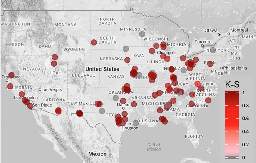
2 Bayesian multivariate time series causal inference
associated with running advertising campaigns for products distributed through brick-
and-mortar retail stores.
The dataset provided by Maxpoint was obtained as follows: MaxPoint ran an adver-
tising campaign at 627 test stores across the United States. An additional 318 stores
were chosen as control stores. Control stores were not targeted in the advertising cam-
paign. The company collected weekly sales data from all of these stores for 36 weeks
before the campaign began and for the 10 weeks in which the campaign was conducted.
The time during which the campaign was conducted is known. The test stores and the
control stores were randomly selected from different economic regions across the U.S..
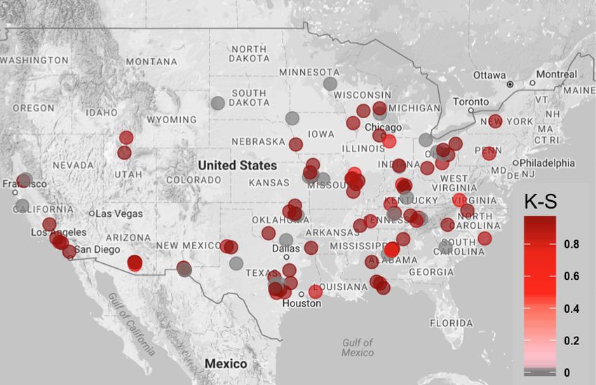
Figure 1 shows an example of the locations of stores in the State of Texas.2
Figure 1: An example of test and control store locations in the State of Texas (Google Maps,
2017). The red dots represent the locations of the test stores; the blue dots represent the
locations of the control stores.
To the best of our knowledge, the work of Brodersen et al. (2015) is the most related
one to the present study. Their method can be described as follows. For each test store,
they first split its time series data into two parts: before and during a causal impact (in
our case, the impact is the advertising campaign). Then, they used the data collected
before the impact to predict the values during the causal period. At the same time, they
applied a stochastic search variable selection (SSVS) method to construct a synthetic
control for that store. The counterfactual potential outcomes (Rubin, 2005) are the sum
of the predicted values and the data from the synthetic control. Clearly, the potential
outcomes of the store exposed to advertising were the observed data. Finally, they
compared the difference between the two potential outcomes and took the average of
differences across different time points. The averaged difference is a commonly used
causal estimand that measures the temporal average treatment effect (Bojinov and
Shephard, 2017).
2 Note:The locations of the stores shown in the figure are not associated with any real datasets
collected by MaxPoint.
imsart-ba ver. 2014/10/16 file: BayesianCausalInference.tex date: March 13, 2018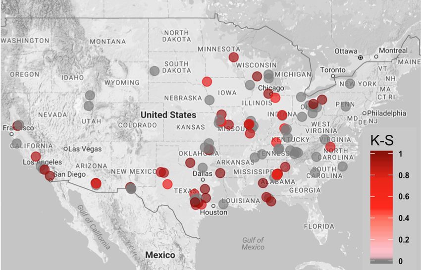
Bo Ning et al.                                                                          3

    The method proposed by Brodersen et al. (2015) is novel and attractive; however,
it cannot directly apply to analyze our dataset due to the following three reasons: (1)
Many causal impacts in our dataset are weak. The causal estimand that Brodersen et al.
(2015) used often fails to detect them; (2) The test stores within an economic region
are spatially correlated as they share similar demographic information. Using Brodersen
et al. (2015)’s method would not allow to consider the spatial correlation between stores;
(3) The SSVS method is computationally slow because it requires sampling from a large
model space consisting of 2p possible combinations of p control stores. In the following,
we will discuss our proposed method for addressing these three difficulties.
    First, we propose a new method for detecting weaker causal impacts. The method
compares two posterior distributions of the latent variables of the model, where one
distribution is computed by conditioning the observed data and the other one is com-
puted by conditioning the counterfactual potential outcomes. We use the one-sided
Kolmogorov-Smirnov (KS) distance to quantify the distance between the two posterior
distributions.
   The new method can successfully detect weaker impacts because it compares two
potential outcomes at the latent variable level; while the commonly used method com-
pares them at the observation level. Since the observed data often contain “inconvenient”
components—such as seasonality and random errors—which inflate the uncertainty of
the estimated causal effect, the commonly used method may fail to detect weaker im-
pacts. In the simulation study, we show that the new method outperforms the commonly
used method even when the model is slightly misspecified.
    The causal estimand in the new method is different from the causal estimand of
the commonly used method. The former one measures the temporal average treatment
effect using the KS distance between two posterior distributions and the latter measures
that effect using the difference between two potential outcomes. Formal definitions of
the two causal estimands are provided in Section 2.
    Secondly, we use a multivariate version of a structural time series model (Harvey
and Peters, 1990) to model the sales data of test stores by allowing pooling of infor-
mation among those stores that locate in geographically contiguous economic regions.
This model enjoys a few advantages that make it especially suitable for our causal in-
ference framework. First, the model is flexible to adapt to different structures of the
latent process. Secondly, it can be written as a linear Gaussian state-space model and
exact posterior sampling methods can be carried out by applying the Kalman filter
and simulation smoother algorithm proposed by Durbin and Koopman (2002, 2012).
Thirdly, it is relatively easy to deal with missing data due to the use of the Kalman fil-
ter and backward smoothing (KFBS) algorithm. The imputing process can be naturally
incorporated into the Markov chain Monte Carlo (MCMC) loop.
    Since test stores are correlated, the number of parameters in the covariance matrix
grows quadratically with the dimension. Consequently, there will not be enough data
to estimate all these parameters. In our approach, we reduce the number of parameters
by imposing sparsity based on a given spatial structure (Smith and Fahrmeir, 2007;
Barber and Drton, 2015; Li et al., 2015). We consider a graphical model structure for

         imsart-ba ver. 2014/10/16 file: BayesianCausalInference.tex date: March 13, 2018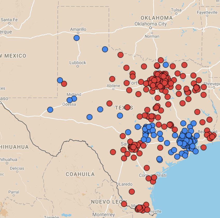
4                             Bayesian multivariate time series causal inference

dependence based on geographical distances between stores. If the distance between two
stores is very large, we treat them conditionally independent given other stores. In terms
of a graphical model, this is equivalent to not put an edge between them. We denote
the corresponding graph by G. Note that G is given in our setting and is completely
determined by the chosen thresholding procedure. We use a graphical Wishart prior
with respect to the given graph G, in short a G-Wishart prior (Roverato, 2002), to
impose sparsity on the precision matrix. One advantage is that this prior is conjugate
for a multivariate normal distribution. If G is decomposable, sampling from a conjugate
G-Wishart posterior is relatively easy due to an available closed form expression for the
normalizing constant in the density (Lauritzen, 1996; Roverato, 2000, 2002). However, if
G is non-decomposable, the normalizing constant does not usually have a simple closed
form (see however; Uhler et al., 2017), and thus one cannot easily sample directly from
its posterior. In such a situation, an approximation for the normalizing constant is
commonly used (Atay-Kayis and Massam, 2005; Mitsakakis et al., 2011; Wang and Li,
2012; Khare et al., 2015). A recent method introduced by Mohammadi and Wit (2015) is
a birth-death Markov chain Monte Carlo (BDMCMC) sampling method. It uses a trans-
dimension MCMC algorithm that transforms sampling of a high-dimensional matrix to
lower dimensional matrices, thus improving efficiency when working with large precision
matrices.
   In a multivariate state-space model, the time dynamics are described by a multi-
variate stochastic trend, usually an order-one vector autoregressive (VAR(1)) process
(de Jong, 1991; de Jong and Chu-Chun-Lin, 1994; Koopman, 1997; Durbin and Koop-
man, 2002). To use a VARMA(p, q) (order p vector autoregression with order q moving
average) with p > 1, q ≥ 0 process is also possible and the choice of p, q can be made
based on data (e.g., chosen by the Bayesian Information Criterion). However, the larger
the p and q are, the larger the number of parameters that need to be estimated. For the
sake of tractability, we treat the hidden process as a VAR(1) process throughout the
paper.
     Putting stationarity constraints on the VAR(1) process is necessary to prevent the
prediction intervals from becoming too wide to be useful. However, constructing an
appropriate prior complying with the constraints is not straightforward. Gelfand et al.
(1992) proposed a naive approach that puts a conjugate prior on the vector autoregres-
sive parameter to generate samples and only keep the samples meeting the constraints.
However, it can be highly inefficient when many draws from the posterior correspond
to nonstationary processes. A simple remedy is to project these nonstationary draws
on the stationarity region to force them to meet the constraints (Gunn and Dunson,
2005). However, the projection method is somewhat unappealing from a Bayesian point
of view because it would make the majority of the projected draws have eigenvalues
lying on the boundary of the corresponding space (Galindo-Garre and Vermunt, 2006;
Roy et al., 2016). We instead follow the recently proposed method of Roy et al. (2016)
to decompose the matrix into several unrestricted parameters so that commonly used
priors can be put on those parameters. While conjugacy will no longer be possible,
efficient algorithms for drawing samples from the posterior distribution are available.
   Thirdly, to accelerate the computational speed of selection control stores, we suggest
using a revised version of the Expectation-Maximization variable selection (EMVS)

         imsart-ba ver. 2014/10/16 file: BayesianCausalInference.tex date: March 13, 2018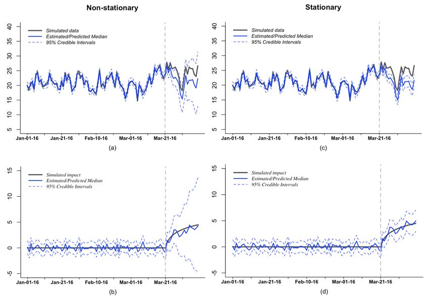
Bo Ning et al.                                                                           5

method (Ročková and George, 2014). The model uses an Expectation-Maximization
(EM) algorithm that is faster and does not need to search 2p possible combinations.
    It is worth mentioning that there are many other popular methods for construct-
ing a synthetic control, such as the synthetic control method proposed by Abadie and
Gardeazabal (2003), the difference-in-differences method (Abadie, 2005; Bonhomme and
Sauder, 2011; Donald and Lang, 2007), and the matching method (Stuart, 2010). More-
over, Doudchenko and Imbens (2016) provided a nice discussion on the advantages and
disadvantages of each method. Unlike these methods, there are two advantages of using
our proposed method: It does not need to have a prior knowledge about the relevant
control stores, the process of selecting control stores is completely driven by data and
can be easily incorporated into a Bayesian framework. It provides a natural model-
based causal inference by viewing counterfactual potential outcomes as missing values
and generating predicting credible intervals from their posterior predictive distributions,
and finally providing a quantitative measure for the strength of the causal effect (Rubin,
2005).
   We apply our method on both simulated datasets and the real dataset provided
by MaxPoint. In the simulation study, we compare the new method with the method
proposed by Brodersen et al. (2015).
    The rest of the paper is organized as follows. Section 2 introduces causal assumptions
and causal estimands. Section 3 describes the model and the priors. Section 4 describes
posterior computation techniques. Section 5 introduces our proposed new approach to
infer causal effects in times series models. Simulation studies are conducted in Section
6. In Section 7, the proposed method is applied on a real dataset from an advertising
campaign conducted by MaxPoint. Finally, Section 8 concludes with a discussion.

2     Causal assumptions and causal estimands
This section includes three parts. First, we will introduce the potential outcomes frame-
work. Secondly, we shall discuss three causal assumptions. Finally, we shall define two
causal estimands, one of them is new.
    The potential outcomes framework is widely used in causal inference literature (Ru-
bin, 1974, 2005; Ding and Li, 2017). Potential outcomes are defined as the values of an
outcome variable at a future point in time after treatment under two different treatment
levels. Clearly, at most one of the potential outcomes for each unit can be observed,
and the rest are missing (Holland, 1986; Rubin, 1977; Imbens and Rubin, 2015). The
missing values can be predicted using statistical methods. In the paper, we predict the
values using the data from a synthetic control that is constructed from several control
stores.
   Based on the potential outcomes framework, we conduct the causal inference. There
are three assumptions need to make for conducting the inference. They are,

    1. The stable unit treatment value assumption (SUTVA);

         imsart-ba ver. 2014/10/16 file: BayesianCausalInference.tex date: March 13, 2018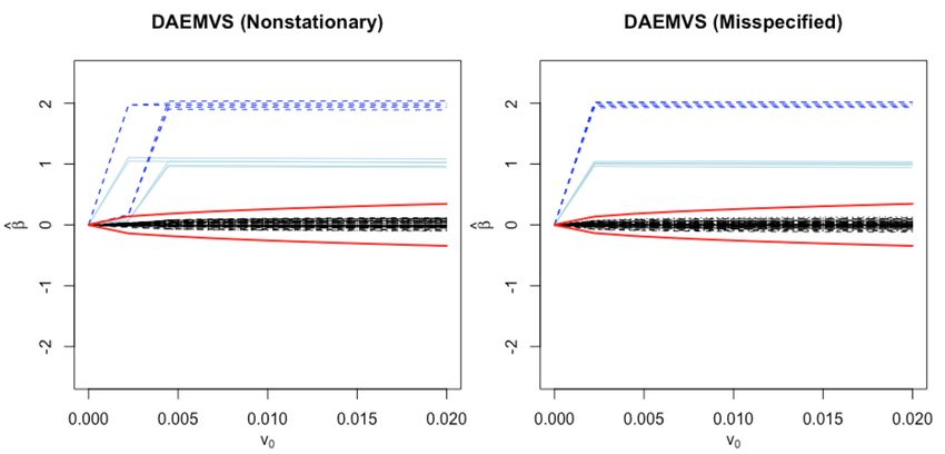
6                                 Bayesian multivariate time series causal inference

    2. The strong ignorability assumption on the assignment mechanism;
    3. The trend stays stable in the absence of treatment for each test store.

    The SUTVA contains two sub-assumptions: no interference between units and no
different versions of a treatment (Rubin, 1974). The first assumption is reasonable be-
cause the stores did not interact with each other after the advertising was assigned.
As Rosenbaum (2007) pointed out, “interference is distinct from statistical dependence
produced by pretreatment clustering.” Since the spatial correlation between test stores
is produced by pretreatment clustering, it is different from the interference between
stores. The second assumption is also sensible because we assume that there are no
multiple versions of the advertising campaign. For example, the advertising campaign
is not launched across multiple channels.
   The strong ignorability assumption also contains two parts: unconfoundedness and
positivity (Ding and Li, 2017). Unconfoundedness means that the treatment is assigned
randomly and positivity means that the probability for each store being assigned is
positive. In our study, we assume the company randomly assigned advertising to stores
and each store has an equal probability of being assigned.
    The last assumption says that the counterfactual potential outcomes in the absence
of the advertising in test stores are predictable.
    Now, we shall introduce some notations before defining causal estimands. Let n be
the total number of test stores to which the advertising were assigned. The i-th test
store has pi control stores (stores did not assigned withPthe advertising), i = 1, . . . , n.
                                                                   n
The total number of control stores are denoted as p, p = i=1 pi . The length of the time
series data is T +P . Let 1, . . . , T be the periods before running the advertising campaign
and T + 1, . . . , T + P be the periods during the campaign. Let wt = (w1t , . . . , wn+p,t )0
be a vector of treatment at time t = T + 1, . . . , T + P , with each wit being a binary
variable. The treatment assignment is time-invariant, so wt = w. For stores assigned
with advertising, we denote the sales value for the i-th store at times t as yit . Let
 obs                                    cf
yit  be the observed data and yit          be the counterfactual potential outcomes which are
                      obs      obs
missing. We let Y t = (y1t , . . . , ynt       ) and Y cf
                                            obs 0              cf           cf 0
                                                        t = (y1t , . . . , ynt ) respectively be the
observed and missing potential outcomes for n test stores at time t, t = 1, . . . , T + P .
Clearly, Y obs
            t    = Y cf                                       obs                  obs         obs
                       t when t = 1, . . . , T . We define Y T +1:T +P = (Y T +1 , . . . , Y T +P )
                                                                                                   0
       cf                cf            cf    0
and Y T +1:T +P = (Y T +1 , . . . , Y T +P ) .
    We first define the causal estimand of a commonly used method. For the i-th test
store, the commonly used causal estimand is defined as
                                        T +P
                                      1 X          obs    cf

                                                  yit  − yit   ,
                                      P
                                         t=T +1

which is the temporal average treatment effects (Bojinov and Shephard, 2017) at P
time points. In our setting, the treatment effects for n test stores are defined as
                                       T +P
                                     1 X
                                                  Y obs − Y cf

                                                    t       t .                               (2.1)
                                     P
                                       t=T +1

          imsart-ba ver. 2014/10/16 file: BayesianCausalInference.tex date: March 13, 2018
Bo Ning et al.                                                                               7

    To introduce our new causal estimand, let xit be the data for the synthetic control
for the i-th test store at time t. Recall that the data of a synthetic control is a weighted
sum of the sales from several control stores. Define X 1:T +P = (X 1 , . . . , X T +P ), where
X t is an n × p matrix containing data from p control stores at time t. Let µit be a latent
variable of a model, which is of interest. Define µt = (µ1t , . . . , µnt ) which is an n × 1
vector. We let
                                   TX
                                    +P
                               p(      µt Y obs
                                             1:T +P , X 1:T +P ).                         (2.2)
                                  t=T +1

be the posterior distribution of the latent variable conditional on Y obs
                                                                        1:T +P and X 1:T +P ,
and
                            TX
                             +P
                         p(       µt Y obs      cf
                                        1:T , Y T +1:T +P , X 1:T +P ).                (2.3)
                            t=T +1

be the distribution conditional on Y cf
                                     1:T +P and X 1:T +P .

    The new causal estimand is defined as the one-sided Kolmogorov-Smirnov (KS)
distance between the two distributions for i-th store, which can be expressed as
                       h   TX
                            +P
                                        obs      cf
                    sup F(     µit ≤ x yi,1:T , yi,T +1:T +P , xi,1:T +P )
                      x
                             t=T +1
                                 TX
                                  +P                                     i
                                                   obs
                          − F(            µit ≤ x yi,1:T +P , xi,1:T +P ) ,
                               t=T +1

where F(·) stands for the corresponding cumulative distribution function. In our setting,
since test stores are spatially correlated, the causal effect of the i-th test store is defined
as
                        h   TX
                             +P
                     sup F(     µit ≤ x Y obs     cf
                                          1:T , Y T +1:T +P , X 1:T +P )
                      x
                             t=T +1
                                                                                         (2.4)
                                 TX
                                  +P                                   i
                          − F(            µit ≤ x Y obs
                                                    1:T +P , X 1:T +P ) .
                                 t=T +1

    A larger value of the one-sided KS distance implies a potentially larger scale of causal
impact. An impact is declared to be significant if the one-sided KS distance is larger
than its corresponding threshold. The threshold is calculated based on several datasets
that are randomly drawn from the posterior predictive distribution of (2.3) (See Section
5 for more details.)
    We would like to mention that although the proposed method is applied to a mul-
tivariate time series model in this paper, even in the context of a univariate model, the
idea of comparing posterior distributions of latent variables appears to be new. Gen-
erally speaking, this idea can be adopted into many other applications with different
Bayesian models as long as these models are described in terms of latent variables.

         imsart-ba ver. 2014/10/16 file: BayesianCausalInference.tex date: March 13, 2018
8 Bayesian multivariate time series causal inference
3 Model and prior
3.1 Model
We consider a multivariate structural time series model given by (to simplify the nota-
tion, we use Y t instead of Y obs
t in the current and the following sections),
Y t = µt + δ t + X t β + t , (3.1)
where Y t , µt , δ t and t are n × 1 vectors standing for the response variable, trend,
seasonality and measurement error respectively. n is the number of test stores, X t is
an n × p matrix containing data from p control stores at time t and β is a sparse p × 1
vector of regression coefficients, where p can be very large. We allow each response in
Y t to have different number of control stores, and write
x11,t · · · x1p1 ,t 0 ··· 0 ··· 0 ··· 0
0 ··· 0 x21,t · · · x2p2 ,t · · · 0 ··· 0
Xt = ,
. . . . . .
. . .
0 ··· 0 0 ··· 0 · · · xn1,t · · · xnpn ,t ,
Pn
with i=1 pi = p. Let γ = (γ1 , . . . , γp ) be the indicator variable such that γj = 1 if and
only if βj 6= 0. t is an independent and identically distributed (i.i.d) error process.
The trend of the time series is modeled as
µt+1 = µt + τ t + ut , (3.2)
where τ t is viewed as a term replacing the slope of the linear trend at time t to allow
for a general trend, and ut is an i.i.d. error process. The process τ t can be modeled as
a stationary VAR(1) process, driven by the equation
τ t+1 = D + Φ(τ t − D) + v t , (3.3)
where D is an n × 1 vector and Φ is an n × n matrix of the coefficients of the VAR(1)
process with eigenvalues having modulus less than 1. If no stationarity restriction is
imposed on τ t , we model it by
τ t+1 = τ t + v t , (3.4)
where v t is an i.i.d. error process.
The seasonal component δ t in (3.1) is assumed to follow the evolution equation
S−2
X
δ t+1 = − δ t−j + wt , (3.5)
j=0
where S is the total length of a cycle and wt is an i.i.d. error process. For example,
for an annual dataset, S = 12 represents the monthly effect while S = 4 represents the
imsart-ba ver. 2014/10/16 file: BayesianCausalInference.tex date: March 13, 2018Bo Ning et al. 9
quarterly effect. This equation ensures that the summation of S time periods of each
variable has expectation zero.
We assume that the residuals of (3.1)–(3.5) are mutually independent and time
invariant, and are distributed as multivariate normals with mean 0n×1 and covariance
matrices Σ, Σu , Σv and Σw respectively.
By denoting parameters αt = (µ0t , τ 0t , δ 0t , · · · , δ 0t−S+2 )0 and η t = (u0t , v 0t , w0t )0 , the
model can be represented as a linear Gaussian state-space model
Yt = zαt + X t β + t , (3.6)
αt+1 = c + T αt + Rη t , (3.7)
where z, c, T and R can be rearranged accordingly based on the model (3.1)–(3.5); and
t ∼ N (0, Σ), η ∼ N (0, Q), Q = bdiag(Σu , Σv , Σw ) are mutually independent; here
and below “bdiag” refers to a block-diagonal matrix with entries as specified. If τ t is a
nonstationary process in (3.3), then we set c = 0.
3.2 Prior
We will now discuss the priors for the parameters in the model. We separate the pa-
rameters into four blocks: the time varying parameter αt , the stationarity constraint
parameters D and Φ, the covariance matrices of the error terms Σ, Σu , Σv and Σw ,
and the sparse regression parameter β.
For the time varying parameter, we give a prior α1 ∼ N (a, P ) with a is the mean
and P is the covariance matrix. For the covariance matrices of the errors, we choose
priors as follows:
Σ−1 ∼ WG (ν, H), Σ−1 2
u ∼ WG (ν, k1 (n + 1)H),
Σ−1
v ∼ WG (ν, k22 (n + 1)H), Σ−1 2
w ∼ WG (ν, k3 (n + 1)H),
where WG stands for a G-Wishart distribution. For the stationarity constraint parameter
D, we choose a conjugate prior D ∼ N (0, I n ).
Putting a prior on the stationarity constraint matrix of a univariate AR(1) process
is straightfoward. However, for the VAR(1) process in (3.3), the stationarity matrix Φ
has to meet the Schur-stability constraint (Roy et al., 2016), that is, it needs to satisfy
|λj (Φ)| < 1, j = 1, . . . , n, where λj stands for the jth eigenvalue. Thus the parameter
space of Φ is given by
Sn = {Φ ∈ Rn×n : |λj (Φ)| < 1, j = 1, . . . , n}. (3.8)
Clearly simply putting a conjugate matrix-normal prior on Φ does not guarantee that
all the sample draws are Schur-stable. We follow Roy et al. (2016)’s method of putting
priors on Φ through a representation as given below.
We first denote τe t = τ t − D, then the Yule-Walker equation for τe t is
U = ΦU Φ0 + Σv , (3.9)
imsart-ba ver. 2014/10/16 file: BayesianCausalInference.tex date: March 13, 201810 Bayesian multivariate time series causal inference
where U = E(e τ t τe 0t ) is a symmetric matrix. Letting f (Φ, U ) = U −ΦU Φ0 , we have that
f (Φ, U ) is a positive definite matrix if and only if Φ ∈ Sn (Stein, 1952). Furthermore,
we have the following proposition:
Proposition 1. [Roy et al. (2016)] Given a positive definite matrix M , there exists
a positive matrix U , and a square matrix Φ ∈ Sn such that f (Φ, U ) = M if and
only if U ≥ M and Φ = (U − M )1/2 OU −1/2 for an orthogonal matrix O with rank
r = rank(U − M ), where (U − M )1/2 and U −1/2 are full column rank square root of
matrices (U − M ) and U −1 .
In view of Proposition 1, given Φ ∈ Sn and an arbitrary value of M , the solution
for U in equation (3.9) is given by
vec(U ) = (I n2 − Φ ⊗ Φ)−1 vec(M ). (3.10)
Letting V = U − M , we have Φ = V 1/2 OU −1/2 , where V is a positive definite matrix,
and O is an orthogonal matrix. The matrix V can be represented by the Cholesky
decomposition V = LΛL0 , where L is a lower triangular matrix and Λ is a diagonal
matrix with positive entries. Thus the number of unknown parameters in V reduces to
n(n − 1)/2+n. The parameter O can be decomposed by using the Cayley representation
O = E ι · [(I n − G)(I n + G)−1 ]2 (3.11)
with E ι = I n − 2ιe1 e01 , ι ∈ {0, 1} and e1 = (1, 0, . . . , 0)0 , where G is a skew-symmetric
matrix. Thus the number of parameters in O is n(n − 1)/2 + 1. By taking the log-
transform, the parameters in Λ can be made free of restrictions. Therefore there are
n2 unrestricted parameters in Φ plus one binary parameter. We put normal priors on
the n2 unrestricted parameters: the lower triangular elements of L, the log-transformed
diagonal elements of Λ and the lower triangular elements of G. For convenience, we
choose the same normal prior for those parameters and choose a binomial prior for the
binary parameter ι.
For the sparse regression parameter β, we chose a spike-and-slab prior with β ∼
N (0, Aγ ), Aγ = diag(a1 , . . . , ap ) with ai = v0 (1 − γi ) + v1 γi , where 0 ≤ v0 < v1 ,
|γ| p−|γ|
Pp to a diagonal matrix with entries as specified; π(γ|θ) = θ (1 − θ)
diag refers with
|γ| = i=1 γi ; θ ∼ Beta(ζ1 , ζ2 ).
4 Posterior computation
We propose a two-stage estimation algorithm to estimate the parameters. In the first
stage, we adopt a fast variable selection method to obtain a point estimator for β. In
the second stage, we plug-in its estimated value and sample the remaining parameters
using an MCMC algorithm.
To conduct the variable selection on β, a popular choice would be using a SSVS
method (George and McCulloch, 1993). The algorithm searches for 2p possible combi-
nations of βi in β using Gibbs sampling under γ = 0 and γ = 1, i = 1, . . . , p. In the
imsart-ba ver. 2014/10/16 file: BayesianCausalInference.tex date: March 13, 2018Bo Ning et al. 11
multivariate setting, this method is computationally very challenging when p is large.
An alternative way is to use the EMVS method (Ročková and George, 2014). This
method uses the EM algorithm to maximize the posterior of β and thus obtain the
estimated model. It is computationally much faster than the SSVS method. Although
SSVS gives a fully Bayesian method quantifying the uncertainty of variable selection
through posterior distributions, the approach is not scalable for our application which
involves a large sized data. Since quantifying uncertainty of variable selection is not an
essential goal, as variable selection is only an auxiliary tool here to aid inference, the
faster EMVS algorithm seems to be a pragmatic method to use in our application.
After obtaining β̂, we plug it into (3.6)–(3.7) and deduct X t β̂ from Y t . We denote
the new data as Ye t , and will work with the following model:
Ye t = zαt + t ,
(4.1)
αt+1 = c + T αt + Rη t .
In the MCMC step, we sample the parameters in the Model (4.1) from their corre-
sponding posteriors. Those parameters include: the time-varying parameters α1:T , the
stationarity constraint parameters D and Φ, the covariance matrices of the residuals
Σ−1 , Σ−1 −1 −1
u , Σv , and Σw .
The details of the algorithm are presented in the supplementary material (Ning
et al., 2018).
The proposed two-stage estimation algorithm is thus summarized as follows:
∗(0) ∗(0)
Stage 1: EMVS step. Choose initial values for β (0) , a1 and P 1 using the revised
EMVS algorithm to find the optimized value for β.
Stage 2: MCMC step. Given Ye t , we sample parameters using MCMC with the
following steps:
(a) Generate αt using the Kalman filter and simulation smoother method.
(b) Generate Φ using the Metropolis-Hastings algorithm.
(c) Generate D.
(d) Generate covariance matrices from their respective G-Wishart posterior den-
sities.
(e) Go to Step (a) and repeat until the chain converges.
Skip Step (b) and (c) if no stationarity restriction is imposed on τ t .
5 A new method to infer causality
In this section, we will introduce our new method to infer causality (in short, “the new
method”) along a commonly used method.
imsart-ba ver. 2014/10/16 file: BayesianCausalInference.tex date: March 13, 201812 Bayesian multivariate time series causal inference
Recall the treatment effects of the commonly used method is defined in (2.1). Since
PT +P cf
t=T +1 Y t is an unobserved quantity, we replace it by its posterior samples from
T +P
p( t=T +1 Y cf obs
P
t |Y 1:T , X 1:T +P ).
The commonly used method may fail to detect even for a moderately sized impact
for two reasons. First, the prediction intervals increase linearly as the time lag increases.
Secondly, the trends are the only latent variables would give a response to an impact,
including the random noise and the seasonality components would inflate the uncer-
tainty of the estimated effect. For the data have a low signal-to-noise ratio, this method
is which even harder to detect causal impacts.
We thus propose a new method by comparing only the posterior distributions of the
latent trend in the model given the observations and the data from counterfactuals. The
new method consists the following five steps:
Step 1: Applying the two-stage algorithm to obtain posterior samples for parameters
in the model using the data from the period without causal impacts.
Step 2: Based on those posterior samples, obtaining sample draws of Y cf T +1:T +P
from its predictive posterior distribution p(Y cf obs
T +1:T +P |Y 1:T , X 1:T +P ).
Step 3: Generating k different datasets from counterfactual potential outcomes (in
short, “counterfactual datasets”) from the predictive posterior distribution, for the j-th
cf(j) cf(j)
dataset, j ∈ {1, . . . , k}, denoted by Y T +1:T +P . Then fitting each Y T +1:T +P into the
model to obtain sample draws of the trend from its posterior distribution, which is
cf(j)
shown in (2.3) (here, we replace Y cf T +1:T +P with Y T +1:T +P ). Also, fitting the observed
data Y obs
1:T +P into the model and sampling from (2.2).
Step 4: Using the one-sided Kolmogorov-Smirnov (KS) distance to quantify the
difference between the posterior distributions of the trend given by the observed data
and the counterfactual datasets. The posterior distribution of the trend given by the
counterfactual datasets is obtained by stacking the sample draws estimated from all
the k simulated datasets. Then calculating the KS distance between the two posterior
distributions for each store as follows:
k
h1 X TX
+P
cf(j)
µit ≤ x Y obs
sup F( 1:T , Y T +1:T +P , X 1:T +P )
x k j=1 t=T +1
(5.1)
TX
+P i
obs
− F( µit ≤ x Y 1:T +P , X 1:T +P ) ,
t=T +1
where i = 1, . . . , n, and F(·) stands for the empirical distribution function of the ob-
tained MCMC samples.
Step 5: Calculating the k × (k − 1) pairwise one-sided KS distances between the
posterior distributions of the trends given by the k simulated counterfactual datasets,
imsart-ba ver. 2014/10/16 file: BayesianCausalInference.tex date: March 13, 2018Bo Ning et al. 13
that is to calculate the following expression
h TX
+P
cf(j)
sup F( µit ≤ x Y obs
1:T , Y T +1:T +P , X 1:T +P )
x
t=T +1
(5.2)
TX
+P
cf(j 0 )
i
obs
− F( µit ≤ x Y 1:T , Y T +1:T +P , X 1:T +P ) ,
t=T +1
where j, j 0 = 1, . . . , k, j 6= j 0 . Then, for each i, choosing the 95% upper percentile
among those distances as a threshold to decide whether the KS distance calculated
from (5.1) is significant or not. If the KS distance is smaller than this threshold, then
the corresponding causal impact is declared not significant.
The use of a threshold is necessary, since the two posterior distributions of the trend
obtained under observed data and the data from the counterfactual are not exactly equal
even when there is no causal impact. Our method automatically selects a data-driven
threshold through a limited repeated sampling as in multiple imputations.
So far we described the commonly used method and the new method in the setting
where the period without a causal impact comes before that with the impact. However,
the new method can be extended to allow datasets in more general situations when: 1)
there are missing data from the period without causal impact; 2) the period without
causal impact comes after the period with a impact; 3) there are more than one periods
without causal impact, both before and after the period with a impact. This is because
the KFBS method is flexible to impute missing values at any positions in a times series
dataset.
6 Simulation study
In this section, we conduct a simulation study to compare the two different methods
introduced in the last section. To keep the analysis simple, we only consider the setting
that the period with causal impact follows that without the impact. We also conduct
convergence diagnostics for MCMC chains and a sensitivity analysis for the new method,
the results are shown in Section 4 of the supplementary material (Ning et al., 2018).
6.1 Data generation and Bayesian estimation
We simulate five spatially correlated datasets, and assume the precision matrices in the
model have the adjacency matrix as follows:
1 1 0 0 0
1 1 1 0 0
0 1 1 1 0 , (6.1)
0 0 1 1 1
0 0 0 1 1
imsart-ba ver. 2014/10/16 file: BayesianCausalInference.tex date: March 13, 201814 Bayesian multivariate time series causal inference
that is, we assume variables align in a line with each one only correlated with its nearest
neighbors. We generate daily time series for an arbitrary date range from January 1,
2016 to April 9, 2016, with a perturbation beginning on March 21, 2016. We specify
dates in the simulation to facilitate the description of the intervention period. We first
generate five multivariate datasets for test stores with varying levels of impact and label
them as Datasets 1–5.
For each Dataset i, i = 1, . . . , 5, the trend is generated from µit ∼ N (0.8µi,t−1 , 0.12 )
with µi0 = 1. The weekly components are generated from two sinusoids of the same
frequency 7 as follows:
δit = 0.1 × cos(2πt/7) + 0.1 × sin(2πt/7). (6.2)
Additional datasets for 10 control stores are generated, each from an AR(1) process
with coefficient 0.6 and standard error 1. We let the first and second datasets to have
regression coefficients β1 = 1, β2 = 2 and let the rest to be 0. We then generate the resid-
uals t in the observation equation from the multivariate normal distribution N (0, Σ)
with precision matrix having sparsity structure given by (6.1). We set the diagonal el-
ements for Σ−1 to 10, and its non-zero off-diagonal elements to 5. The simulated data
for test stores are the sum of the simulated values of µt , δ t , X t β and t . The causal
impacts are generated as follows: for each Dataset i, i = 1, . . . , 5, we add an impact
scale (i−1)
2 × (log 1, . . . , log 20) from March 21, 2016 to April 9, 2016. Clearly no causal
impact is added in Dataset 1.
We impose the graphical structure with adjacency matrix in (6.1) in both observed
and hidden processes in the model and then apply the two-stage algorithm to estimate
parameters. In Stage 1, we apply the revised EMVS algorithm. We choose the initial
∗(0) ∗(0)
values β (0) and a1 to be the zero vectors and the first 15×15 elements of P 1 , which
correspond to the covariances of the trend, local trend and seasonality components, to
∗(0)
be a diagonal matrix. The remaining elements in P 1 are set to 0. We select 20 equally
−6
spaced relatively small values for v0 from 10 to 0.02 and a relatively larger value for
v1 , 10. For the prior of θ, we set ζ1 = ζ2 = 1. The maximum number of iterations of
the EMVS algorithm is chosen to be 50. We calculate the threshold of non-zero value
of β i from the inequality: p(γi = 1|βi , Y ∗t , X ∗t ) > 0.5 (See the detailed discussions in
Ročková and George, 2014). Then the threshold can be expressed as
s
log(v0 /v1 ) + 2 log(θ̂/(1 − θ̂))
|βith | ≥ ,
v1−1 − v0−1
where θ̂ is the maximized value obtained from the EMVS algorithm. Ročková and George
(2014) also suggested using a deterministic annealing variant of the EMVS (DAEMVS)
algorithm which maximizes
1
log π(α∗1:T , β, γ, θ, Φ, Σ, Q|Y ∗t , X ∗t )s | β (k) , θ(k) , Φ(k) , Σ(k) , Q(k) , (6.3)
E(α∗1:T ,γ)|·
s
where 0 ≤ s ≤ 1. The parameter 1/s is known as a temperature function (Ueda and
Nakano, 1998). When the temperature is higher, that is when s → 0, the DAEMVS
imsart-ba ver. 2014/10/16 file: BayesianCausalInference.tex date: March 13, 2018Bo Ning et al. 15
Figure 2: EMVS (left) and DAEMVS (with s = 0.1) (right) estimation of β based on the
simulated datasets. The dark blue lines are the parameters that have simulated values 2; the
light blue lines are the parameters that have simulated values 1 and the black lines are the
parameters that have simulated values 0. The red lines are the calculated βith values, within
the two red lines, the parameters should be considered as zero parameters.
algorithm has a higher chance to find a global mode and thus reduces the chance of
getting trapped at a local maximum.
Figure 2 compares the results for using EMVS and DAEMVS with s = 0.1 algo-
rithms. We plot β̂ and their thresholds based on 20 different values of v0 from 10−6
to 0.02. From the plot, the estimated values for β using both EMVS and DAEMVS
methods are close to their true values.
The true zero coefficients are estimated to be very close to 0. However, we observe
that the values of βith is larger by using the EMVS method compared to the DAEMVS
method. This is because in the region where v0 is less than 0.005, the
θ̂ estimated from
EMVS is very close to 0, thus the negative value of log θ̂/(1 − θ̂) is very large and
the threshold becomes larger. Based on the simulation results, we use DAEMVS with
s = 0.1 throughout the rest of the paper.
The DAEMVS gives a smaller value of βith , yet the thresholds can distinguish the
true zero and non-zero coefficients in this case. Nevertheless it may miss a non-zero
coefficient if the coefficent is within the thresholds. In practice, since our goal is to
identify significant control variables and use them to build counterfactuals for a causal
inference, we may choose to include more variables than the threshold suggests provided
that the total number of included variables is still manageable.
Recall that in the Stage 1, we used a conjugate prior for vec(Φ) instead of the
originally proposed prior described in Section ??. Here, we want to make sure the
imsart-ba ver. 2014/10/16 file: BayesianCausalInference.tex date: March 13, 201816 Bayesian multivariate time series causal inference
change of prior would not affect the results of β̂ too much. We conduct the analysis by
choosing two different values of the covariance matrix of the prior: I 5 and 0.01 × I 5 .
We found the estimates β̂s are almost identical to the estimated values shown in Figure
2. We also consider using other two models: one ignores the stationarity constraint for
τ t (henceforth the “nonstationary model”); another ignores the time dependency of the
model (henceforth the “misspecified model”). To be more explicit, for the nonstaionary
model, we let the local linear trend follow (3.4). The misspecified model is given by
Y ∗t = X ∗t β + ς t , with ς t s are i.i.d random errors with multivariate normally distributed
and mean 0 by ignoring their dependency. We conduct DAEMVS with s = 0.1 for both
of the two models. In the nonstationary model, we choose a diffuse prior for α∗1 and
∗(0)
change the covariance corresponding to the local linear trend in P 1 to be 106 × I 5 .
In the misspecifed model, the M-step can be simplified to only updates for β, θ and
the covariance matrix of ς t . We plot the results into Figure 3. Comparing the results
in Figure 3 with Figure 2, there are not much differences among the results obtained
using the three different models for estimating β.
Figure 3: DAEMVS (with s = 0.1) estimation of β based on the simulated datasets using
the nonstationary model (left) and the misspecified model (right). The dark blue lines are the
parameters that have simulated values 2; the light blue lines are the parameters that have
simulated values 1 and the black lines are the parameters that have simulated values 0. The
red lines are the calculated βith values, within the two red lines, the parameters should be
considered as zero.
In Stage 2, we plug-in β̂ and calculate Ye t in (4.1). We choose the prior for the rest of
parameters as follows: we let α1 ∼ N (0, I). If τ t is a nonstationarity process, the initial
condition is considered as a diffuse random variable with large variance (Durbin and
Koopman, 2002). Then we let the covariance matrix of τ t to be 106 × I 5 . We let ν = 1,
k1 = k2 = k3 = 0.1. We choose H = I 5 and the priors for 25 parameters decomposed
imsart-ba ver. 2014/10/16 file: BayesianCausalInference.tex date: March 13, 2018Bo Ning et al. 17
√ 2
from Φ to be N (0, 5 ), and let ι ∼ Bernoulli(0.5). We run total 10, 000 MCMC
iterations with the first 2, 000 draws as burn-in. An MCMC convergence diagnostic
and a sensitive analysis of the model are conducted, we include their results in the
supplementary file.
6.2 Performance of the commonly used causal inference method
In this section, we study the performance of the commonly used method. The causal
effect is estimated by taking the difference between observed data during causal period
and the potential outcomes of counterfactuals during that period. In Stage 1, we use the
DAEMVS (s = 0.1) algorithm to estimate β̂ for the model (3.6)–(3.7). A stationarity
constraint is added on the local linear trend τ t . In Stage 2, we consider two different
settings for τ t : with and without adding the stationarity constraint. We choose Dataset
4 as an example and plot accuracy of the model based on the two different settings in
Figure 4. There are four subplots: the left two subplots are the results for the model
with a nonstationary local linear trend and the right two subplots are the results for the
model with a stationary local linear trend. Before the period with a causal impact, which
is March, 21, 2016, the estimated posterior medians and 95% credible intervals obtained
from the two models are close (see plots (b) and (d) in Figure 4); but their prediction
intervals during the period with a causal impact are quite different. In the model with
a nonstationary local linear trend, the prediction intervals are much wider and expand
more rapidly than those resulting from the model with a stationary local linear trend.
In the former case, the observed data during the campaign are fully contained inside the
prediction intervals and thus failed to detect a causal impact. However, the model with
a stationary local linear trend gives only moderately increasing prediction intervals and
thus can detect the causal impact. Plots (b) and (d) shown in the bottom of Figure 4
are the estimated causal impact in each model for Dataset 4 calculated by taking the
difference between observed values and counterfacutal potential outcomes. In each plot,
the estimated causal impact medians are able to capture the shape of the simulated
causal impact. However, the prediction intervals in plot (b) contain the value 0 and
thus negate the impact. The shorter prediction intervals in plot (d) do not contain the
value 0, and thus indicate the existence of a impact.
To give an overall picture of the model fitting for the five simulated datasets, we
summarize the posterior medians and their 95% credible intervals of the estimated
causal impact for all the datasets in Table 1. In the model with a nonstationary local
linear trend, no impacts are detected for all the five datasets since their corresponding
prediction intervals all contain the value 0. In the model with a stationary local linear
trend on τ t , the impacts are successfully detected for the last three datasets. For Dataset
2, it has a weaker impact. Its impact is not detected even after imposing the stationarity
constraint. Also, when the stationarity constraint is imposed, including the intercept D
in (3.3) helps give a robust long run prediction. Thus, from Table 1, we find that the
estimated medians using the model with a stationary local linear trend are closer to the
true impact compared with that obtained from using the model with a nonstationary
local linear trend.
imsart-ba ver. 2014/10/16 file: BayesianCausalInference.tex date: March 13, 201818 Bayesian multivariate time series causal inference
Figure 4: Plot of the causal impact in Dataset 4 using models with a stationary and a non-
stationary local linear trend. (a) and (c) are the plots of estimation (before March 21, 2016)
and prediction (after March 21, 2016) of Dataset 4 without stationarity constraint (left) and
with stationarity constraint (right). The gray line is the simulated dataset, the blue line is the
estimated posterior median of the dataset using the model, the dashed blue line is the corre-
sponding 95% credible and prediction intervals. (b) and (d) are the plots of estimated causal
impact by taking the difference between the observed data and Bayesian estimates using the
model with a nonstationary local linear trend (left) and the model with a stationary local
linear trend (right). The black line is the simulated true impact, the blue line is the estimated
median of the impact, the dashed blue lines are the corresponding 95% credible and prediction
intervals.
In the setting where the sales in the test stores are spatially correlated, the use of
the multivariate model with a stationary local linear trend is necessary for obtaining
more accurate estimates for causal effects. We compare the results with a univariate
model which ignores the correlation between the five simulated datasets. We fit the
five datasets independently into that model. The model is the univariate version of
the model (3.6)–(3.7). In the univariate model, the errors t , ut , v t and wt become
scalars. We denote σ 2 , σu2 , σv2 and σw 2
as their corresponding variances. We choose their
priors as σ −2 ∼ Gamma( 2 , 2 ), σu−2 , σv−2 , σw
0.1 0.1×SS −2
∼ Gamma(0.01, 0.01 × SS), where
imsart-ba ver. 2014/10/16 file: BayesianCausalInference.tex date: March 13, 2018Bo Ning et al. 19
Table 1: Posterior medians and 95% credible intervals of average causal impacts for simulated
datasets estimated using the multivariate models with a stationary and a nonstationary local
linear trend.
Simulated impact Nonstationary Stationary
Dataset 1 0.00 0.00 [−4.419, 4.425] 0.29 [−1.440, 1.996]
Dataset 2 1.06 0.64 [−3.989, 5.298] 1.07 [−0.648, 2.780]
Dataset 3 2.12 1.22 [−3.758, 5.965] 2.27 [0.399, 4.014]
Dataset 4 3.18 2.83 [−1.793, 7.575] 3.16 [1.500, 4.862]
Dataset 5 4.23 4.25 [−0.249, 8.771] 4.25 [2.520, 5.904]
Table 2: Posterior medians and 95% credible intervals of average causal impacts for simulated
datasets estimated using the univariate model.
Simulated impact Stationary (univariate)
Dataset 1 0.00 0.17 [−2.197, 2.472]
Dataset 2 1.06 1.03 [−1.365, 3.473]
Dataset 3 2.12 2.16 [−0.370, 4.476]
Dataset 4 3.18 3.20 [0.821, 5.748]
Dataset 5 4.23 4.08 [1.564, 6.489]
PT PT
SS = t=1 (yt − ȳ)2 /(T − 1) and ȳ = t=1 yt /T . The parameters D and Φ in (3.3)
also become scalars and to be denoted by d and φ respectively. We give them the priors
d ∼ N (0, 0.12 ) and φ ∼ N (0, 0.12 )1(−1,1) .
In order to make the comparison between the multivariate model and the univariate
model meaningful, we plug-in the same β̂ obtained from Stage 1 for both models. We
conduct an MCMC alogrihtm for the five datasets separately using the univariate model
by sequentially sampling draws from the corresponding posterior distributions of α1:T ,
2
d, φ, σ 2 , σu2 , σv2 and σw . We run the MCMC algorithm for 10,000 iterations and treat
the first 2,000 as burn-in. The estimated causal impacts are shown in Table 2. By
comparing the results with the results in Table 1, the univariate model produces wider
credible intervals for all of datasets even though their posterior medians are close to the
truth. Thus the multivariate model with a stationary local linear trend is more accurate
for detecting a causal impact.
We conduct additional independent 10 simulation studies by generating datasets
using the same scheme which described above, but using different random number gen-
erators from the software. We conduct the same analysis for the 10 simulated studies
using the multivariate model with stationarity constraints. All of these studies show
that the commonly used method failed to detect causal effect for the second dataset,
which is the one with the smallest amount of simulated causal impact.
6.3 Performance of the new method to infer causality
In this section, we study the performance of the new method. We use the same simulated
data in Section 6.1. We calculate the one-sided KS distance in (5.1) and the threshold
imsart-ba ver. 2014/10/16 file: BayesianCausalInference.tex date: March 13, 201820 Bayesian multivariate time series causal inference
in (5.2) for each i = 1, . . . , n. We also calculate the one-sided KS distances
k
h1 X TX
+m
cf(j)
µit ≤ x|Y obs
sup F( 1:T , Y T +1:T +m , X 1:T +m )
x k j=1 t=T +1
TX
+m i
− F( µit ≤ x|Y obs
1:T +m , X 1:T +m )
t=T +1
and the corresponding thresholds for m = 1 to m = P . This allows to see how the KS
distances grow over time.
We plot the results in Figure 5. There are five subplots in that figure with each
represents one simulated dataset. For each subplot, the red line represents the one-
sided KS distances between posteriors from a test store and its counterfactuals, and the
lightblue line represents its corresponding thresholds. The threshold is calculated based
on k = 30 simulated counterfactual datasets. In the plot, Dataset 1 is the only one
with the one-sided KS distances completely below the thresholds and it is the dataset
which does not receive any impacts. This suggests that our method has successfully
distinguished between impact and no impact in these datasets. For Dataset 2, the impact
at the early period is small, thus we observe the causal impact in the first three predicting
periods are not significant; however, the new method can detect the impact after the
fourth period.
We also summarized the results in Table 3. Compared with the results from the
commonly used method (see Table 1), the new method shows a significant improvement
in detecting causal impacts. From Dataset 3 to Dataset 5, the one-sided KS distances
are all above their corresponding thresholds. Also, as the impact grows stronger, we
observe that the distances becomes larger. The thresholds too increase along the time,
since the predicting intervals for the trends become wider.
To check the performance of the new method, we conduct 10 more simulation studies
using the data generated from the same model. Although the values of the one-sided
KS distances and thresholds are not identical for each simulation, since the model is
highly flexible and the estimated trend is sensitive to local changes of a dataset, the
new method successfully detects the causal impacts in Dataset 2, . . . , Dataset 5.
We applied the new method to the univariate model, which is described in Section
6.2, using the same simulated dataset. The graphical and tabular representations of
the results are presented in Section 3 of the supplementary material. We found that
by comparing with the results obtained from the multivariate model (see Figure 5),
the thresholds are much larger among all the datasets. Recall that from Table 2, the
credible intervals estimated using the commonly used method are wider. Thus when
we randomly draw samples from a counterfactual with a larger variance, the posterior
distributions for their trend are more apart. As a result, the pairwise one-sided KS
distances between the posterior distributions of the trends are larger. Even though the
thresholds are larger when using the univariate model, unlike the results obtained by
using the commonly used method, the new method can still detect the causal impact
for almost all the datasets which received an impact successfully, except for the very
imsart-ba ver. 2014/10/16 file: BayesianCausalInference.tex date: March 13, 2018Bo Ning et al. 21
Dataset 1 Dataset 2 Dataset 3
1.0
1.0
1.0
● ●
●
●
●
0.8
0.8
0.8
●
●
● ●
● ●
● ●
● ●
●
K−S distance
K−S distance
K−S distance
● ●
0.6
0.6
0.6
● ●
●
● ● ●
● ● ●
● ● ●
● ● ●
●
0.4
0.4
0.4
● ● ● ●
● ● ● ● ●
● ● ● ● ●
● ● ● ●
● ● ● ● ● ● ● ● ● ● ● ● ● ●
● ● ● ● ● ● ●
0.2
0.2
0.2
● ● ● ● ● ●
● ● ● ● ● ● ● ● ●
● ● ● ● ● ● ● ● ●
●
● ● ● ● ●
● ● ●
●
● ● ●
●
● ● ● ●
0.0
0.0
0.0
● ● ● ●
Mar−22−16 Mar−28−16 Apr−03−16 Apr−09−16 Mar−22−16 Mar−28−16 Apr−03−16 Apr−09−16 Mar−22−16 Mar−28−16 Apr−03−16 Apr−09−16
Dataset 4 Dataset 5
1.0
1.0
● ● ● ● ● ● ● ● ● ● ● ● ●
● ● ● ● ● ●
● ● ●
●
● ●
0.8
0.8
● ●
●
●
●
K−S distance
K−S distance
● ● ●
0.6
0.6
● ● ● ●
●
●
● ● ●
●
0.4
0.4
● ● ●
● ● ● ●
● ●
● ● ● ● ● ● ●
● ● ●
●
● ● ●
0.2
●
0.2
● ● ● ● ●
●
● ● ● ● ●
●
●
0.0
0.0
Mar−22−16 Mar−28−16 Apr−03−16 Apr−09−16 Mar−22−16 Mar−28−16 Apr−03−16 Apr−09−16
Figure 5: Results of applying the new method to detect causal impacts in Dataset 1, . . . ,
Dataset 5 using the multivariate model with a stationary local linear trend during the causal
period from March, 22, 2016 to April, 9, 2016. In each subplot, the red line gives the one-sided
KS distances between two posterior distributions with one is given the data of counterfactuals;
the light blue line gives the corresponding thresholds.
Table 3: Results of the one-sided KS distances and thresholds obtained by applying the new
method to detect causal impacts in Dataset 1, . . . , Dataset 5 using the multivariate model
with a stationary local linear trend. We only present the results at the dates March 22, 2016,
March 31, 2016 and April. 9, 2016 which correspond to the 1st day, 10th day and 20th day
during the causal period.
Dataset 1 Dataset 2 Dataset 3 Dataset 4 Dataset 5
March, 22 KS distance 0.005 0.033 0.103 0.137 0.277
(1st day) Threshold 0.118 0.083 0.112 0.110 0.120
March, 31 KS distance 0.143 0.402 0.612 0.884 0.989
(10th day) Threshold 0.313 0.192 0.256 0.299 0.369
April, 9 KS distance 0.520 0.763 0.928 0.999 1.000
(20th day) Threshold 0.715 0.349 0.354 0.409 0.636
imsart-ba ver. 2014/10/16 file: BayesianCausalInference.tex date: March 13, 2018You can also read