Data-Efficient Learning for Complex and Real-Time Physical Problem Solving using Augmented Simulation
←
→
Page content transcription
If your browser does not render page correctly, please read the page content below

Data-Efficient Learning for Complex and Real-Time Physical Problem
                                                           Solving using Augmented Simulation
                                               Kei Ota1 , Devesh K. Jha2 , Diego Romeres2 , Jeroen van Baar2 , Kevin A. Smith3 , Takayuki Semitsu1 ,
                                                           Tomoaki Oiki1 , Alan Sullivan2 , Daniel Nikovski2 , and Joshua B. Tenenbaum3
                                                1 Mitsubishi Electric, 2 Mitsubishi Electric Research Labs, 3 Massachusetts Institute of Technology

                                            Abstract— Humans quickly solve tasks in novel systems
                                         with complex dynamics, without requiring much interaction.
arXiv:2011.07193v2 [cs.LG] 16 Feb 2021

                                         While deep reinforcement learning algorithms have achieved
                                         tremendous success in many complex tasks, these algorithms
                                         need a large number of samples to learn meaningful policies.
                                         In this paper, we present a task for navigating a marble to the
                                         center of a circular maze. While this system is very intuitive
                                         and easy for humans to solve, it can be very difficult and
                                         inefficient for standard reinforcement learning algorithms to
                                         learn meaningful policies. We present a model that learns to
                                         move a marble in the complex environment within minutes of
                                         interacting with the real system. Learning consists of initializing   Fig. 1: We train a reinforcement learning agent that initializes
                                         a physics engine with parameters estimated using data from            a policy with a general purpose physics engine, then corrects
                                         the real system. The error in the physics engine is then              its dynamics model using parameter estimation and residual
                                         corrected using Gaussian process regression, which is used
                                         to model the residual between real observations and physics           learning. The agent uses this augmented model in a circular
                                         engine simulations. The physics engine augmented with the             maze to drive a marble to the center.
                                         residual model is then used to control the marble in the maze
                                         environment using a model-predictive feedback over a receding
                                         horizon. To the best of our knowledge, this is the first time that
                                         a hybrid model consisting of a full physics engine along with         have internal models of physics that are well calibrated to the
                                         a statistical function approximator has been used to control a        world [7], [8], and that they use these models to learn how to
                                         complex physical system in real-time using nonlinear model-           use new objects to accomplish novel goals in just a handful
                                         predictive control (NMPC).
                                                                                                               of interactions [9]. Thus, we suggest that any agent that can
                                                               I. I NTRODUCTION                                perform flexible physical problem solving should have both
                                            Artificial Intelligence has long had the goal of designing         prior knowledge of the dynamics of the world, as well as a
                                         robotic agents that can interact with the (complex) physical          way to augment those dynamics in a way that supports their
                                         world in flexible, data-efficient and generalizable ways [1], [2].    interactions with the scene. Note that we do not suggest that
                                         Model-based control methods form plans based on predefined            this specific approach corresponds to the way that humans
                                         models of the world dynamics. However, although data-                 learn or reason about physics, but instead that we believe
                                         efficient, these systems require accurate dynamics models,            augmented simulation is key to human sample efficiency, and
                                         which may not exist for complex tasks. Model-free methods             therefore should be important for robotic sample efficiency
                                         on the other hand rely on reinforcement learning, where the           as well. Fig. 1 provides an idea of the proposed approach.
                                         agents simultaneously learn a model of the world dynamics                Our testbed for this problem is a circular maze environment
                                         and a control policy [3], [4]. However, although these                (CME; see Fig. 1), in which the goal is to tip and tilt the
                                         methods can learn policies to solve tasks involving complex           maze so as to move a marble from an outer ring into an inner
                                         dynamics, training these policies is inefficient, as they require     circle. This is an interesting domain for studying real-time
                                         many samples. Furthermore, these method are typically not             control because it is intuitively easy to pick up for people —
                                         generalizable beyond the trained scenarios.                           even children play with similar toys without prior experience
                                            Our aim in this paper is to combine the best of both               with these mazes — and yet is a complex learning domain for
                                         methodologies: our system uses nonlinear model predictive             artificial agents due to its constrained geometry, underactuated
                                         control with a predefined (inaccurate) model of dynamics              control, nonlinear dynamics, and long planning horizon with
                                         at its core, but updates that model by learning residuals             several discontinuities [10], [11]. Adding to this challenge,
                                         between predictions and real-world observations via physical          the CME is a system that is usually in motion, so planning
                                         parameter estimation and Gaussian process regression [5].             and control must be done in real-time, or else the ball will
                                         We take inspiration from cognitive science for this approach,         continue to roll in possibly unintended ways.
                                         as people can interact with and manipulate novel objects well            The learning approach we present in this paper falls
                                         with little or no prior experience [6]. Research suggests people      under the umbrella of Model-Based Reinforcement Learning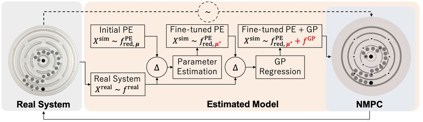
(MBRL). In MBRL, a task-agnostic predictive model of             learning in physical systems has also been studied in the
the system dynamics is learned from exploration data. This       past [20], [21], [22], [11], [23]. However, most of these studies
model is then used to synthesize a controller which is used      use prior physics information in the form of differential
to perform the desired task using a suitable cost function.      equations, which requires domain expertise and thus the
The model in our case is represented by a physics engine         methods also become very domain specific. While we rely
that roughly describes the CME with its physical properties.     on some amount of domain expertise and assumptions, using
Additionally, we learn the residual between the actual system    a general purpose physics engine to represent the physical
and the physics system using Gaussian process regression [5].    system will allow for more readily generalization across a
Such an augmented simulator – a combination of a physics         wide range of systems.
engine and a statistical function approximator – allows us          A similar CME has been solved with MBRL and deep
to efficiently learn models for physical systems while using     reinforcement learning, in [11] and [10], respectively. In [11],
minimal domain knowledge.                                        the analytical equations of motion of the CME have been
   Contributions. Our main contributions are as follows:         derived to learn a semi-parametric GP model [24], [25] of
   • We present a novel framework where a hybrid model           the system, and then combined with an optimal controller.
     consisting of a full physics engine augmented with a        In [10], a sim-to-real approach has been proposed, where a
     machine learning model is used to control a complex         policy to control the marble(s) is learned on a simulator from
     physical system using NMPC in real time.                    images, and then transferred to the real CME. However, the
   • We demonstrate that our proposed approach leads to          transfer learning still requires a large amount of data from
     sample-efficient learning in the CME: our agent learns to   the real CME.
     solve the maze within a couple of minutes of interaction.      While approaches that combine physical predictions and
We have released our code for the CME as it is a complex,        residuals have been used for control in the past [26], here we
low-dimensional system that can be used to study real-time       demonstrate that this combination can be used as part of a
physical control1 .                                              model-predictive controller (MPC) of a much more complex
                                                                 system in real-time. An important point to note here is that the
                      II. R ELATED W ORK                         work presented in [26] uses MPC in a discrete action space,
   Our work is motivated by the recent advances in (deep)        whereas for the current system we have to use nonlinear
reinforcement learning to solve complex tasks in areas such as   model-predictive control (NMPC) that requires a solution to
computer games [12] and robotics [3], [13]. While these algo-    a nonlinear, continuous control problem in real-time (which
rithms have been very successful for solving simulated tasks,    requires non-trivial, compute-expensive optimization) [27].
their applicability in real systems is sometimes questionable    Consequently, the present study deals with a more complicated
due to their relative sample inefficiency. This has motivated    learning and control problem that is relevant to a wide range
a lot of research in the area of transferring knowledge from     of robotic systems.
a simulation environment to the real world [14], [15], [16],                    III. P ROBLEM F ORMULATION
[10]. However, most of these techniques end up being very
                                                                     We consider the problem of moving the marble to the center
data intensive. Here we attempt to study complex physical
                                                                 of the CME. Our goal is to study the sim-to-real problem in
puzzles using model-based agents in an attempt to learn to
                                                                 a model-based setting where an agent uses a physics engine
interact with the world in a sample-efficient manner.
                                                                 as its initial knowledge of the environment’s physics. Under
   Recently the robotics community has seen a surge in
                                                                 these settings, we study and attempt to answer the following
interest in the use of general-purpose physics engines which
                                                                 questions in the present paper.
can represent complex, multi-body dynamics [17]. These
engines have been developed with the intention to allow              1) What is needed in a model-based sim-to-real architec-
real-time control of robotic systems while using them as                ture for efficient learning in physical systems?
an approximation of the physical world. However, these               2) How can we design a sim-to-real agent that behaves
simulators still cannot model or represent the physical system          and learns in a data-efficient manner?
accurately enough for control, and this has driven a lot of          3) How does the performance and learning of our agent
work in the area of sim-to-real transfer [18], [19]. The goal           compare against how humans learn to solve these tasks?
of these methods is to train an agent in simulation and then     We use the CME as our test environment for the studies
transfer them to the real system using minimum involvement       presented in this paper. However, our models and controller
of the real system during training. However, most of these       design are general-purpose and thus, we expect the proposed
approaches use a model-free learning approach and thus tend      techniques could find generalized use in robotic systems. For
to be sample inefficient. In contrast, we propose a method       the rest of the paper, we call the CME together with the tip-
that trains a MBRL sim-to-real agent and thus achieves very      tilt platform the circular maze system (CMS). At this point,
good sample efficiency.                                          we would like to note that we make some simplifications for
   The idea of using residual models for model correction, or    the CMS to model actuation delays and tackle discontinuities
hybrid learning models for control of physical systems during    for controller design as we describe in the following text.
                                                                     The goal of the learning agent is to learn an accurate model
  1 https://www.merl.com/research/license/CME                    of the marble dynamics, that can be used in a controller,
π(uk |xk ), in a model-predictive fashion which allows the comes from a physics engine. The proposed approach is
CMS to choose an action uk given the state observation shown as a schematic in Fig. 2.
xk to drive a marble from an initial condition to the target We want to design a sim-to-real agent, which can bridge
state. We assume that the system is fully defined by the the gap between the simulation environment and the real
combination of the state xk and the control inputs uk , and world in a principled fashion. The gap between the sim-
it evolves according to the dynamics p(xk+1 |xk , uk ) which ulated environment and the real world can be attributed
are composed of the marble dynamics in the maze and the to mainly two factors. First, physics engines represent an
tip-tilt platform dynamics. approximation of the physics of the real systems, because
As a simplification, we assume that the marble dynamics is they are designed based on limited laws of physics, domain
independent of the radial dynamics in each of the individual knowledge, and convenient approximations often made for
rings, i.e., we quantize the radius of the marble position mathematical tractability. Second, there are additional errors
into the 4 rings of the maze. We include the orientation of due to system-level problems, such as observation noise and
the tip-tilt platform as part of the state for our dynamical delays, actuation noise and delays, finite computation time
system, obtaining a five-dimensional state representation for to update controllers based on observations, etc.
the system, i.e., x = (rd , β, γ, θ, θ̇, ). It can be noted that Consequently, we train our agent by first estimating the
the radius rd is a discrete variable, whereas the rest of the parameters of the physics engine, and then compensate for the
state variables are continuous. The terms β, γ represent the different system-level problems as the agent tries to interact
X and Y -orientation of the maze platform, respectively, and with the real system. Finally, Gaussian process Regression
θ, θ̇ represent the angular position and velocity of the marble, is used to model the residual dynamics of the real system
measured with respect to a fixed frame of reference. Since that cannot be described by the best estimated parameters of
rd is fixed for each ring of the CME, we remove rd from the physics engine. In the rest of this section, we describe
the state representation of the CMS for the rest of the paper. the details of the physics engine for the CME, and provide
Thus, the state is represented by a four-dimensional vector our approach for correcting the physics engine as well as
x = (β, γ, θ, θ̇). The angles β, γ are measured using a laser modeling other system-level issues with the CMS.
sensor that is mounted on the tip-tilt platform (see Figure 1)
A. Physics Engine Model Description
while the state of the ball could be observed from a camera
mounted above the CMS. For more details, interested readers As described earlier, we use MuJoCo as our physics engine,
are referred to [11]. f PE . Note that in our model we ignore the radial movement
We assume that there is a discrete planner, which can return of the marble in each ring, and describe the state only with
a sequence of gates that the marble can then follow to move the angular position of the marble as described in Sec. III.
to the center. Furthermore, from the human experiments we Consequently, we restrict the physics engine to consider only
have observed that human subjects always try to bring the the angular dynamics of the marble in each ring, i.e., the
marble in front of the gate, and then tilt the CME to move it radius of the marble position is fixed. However, in order
to the next ring. Therefore, we design a lower level controller to study the performance of the agent in simulation, we
to move the marble to the next ring when the marble is placed also create a full model of the CME where the marble does
in front of the gate to the next ring. Thus, the task of the not have the angular state constraint. Thus, we create two
PE
learned controller is to move the marble in a controlled way different physics engine models: fred represents the reduced
PE
so that it can transition through the sequence of gates to reach physics engine available to our RL model, and ffull uses the
PE PE
the center of the CME. This makes our underlying control full internal state of the simulator. fred differs from ffull in
PE
problem tractable by avoiding discontinuities in the marble two key ways. In the forward dynamics of the fred model,
movement (as the marble moves from one ring to the next). we set the location of the marble to be in the center of each
Before describing our approach, we introduce additional ring because we cannot observe the accurate radial location
PE
nomenclature we will use in this paper. We represent the of the marble in the real system, while this is tracked in ffull .
physics engine by f PE , the residual dynamics model by f GP , Additionally, because we cannot observe the spin of the ball
PE
and the real system model by f real , such that f real (xk , uk ) ≈ in real experiments, we do not include it in fred , while it is
PE PE
f PE (xk , uk ) + f GP (xk , uk ). We use MuJoCo [17] as the included in ffull . We use this ffull model for analyzing the
physics engine, however, we note that our approach is agnostic behavior of our agent in the preliminary studies in simulation.
to the choice of physics engine. In the following sections, we This serves as an analog to the real system in the simulation
describe how we design our sim-to-real agent in simulation, studies we present in the paper. We call this set of experiments
as well as on the real system. sim-to-sim. These experiments are done to determine whether
the agent can successfully adapt its physics engine when
IV. A PPROACH initialized with an approximation of a more complicated
Our approach for designing the learning agent is inspired environment.
by human physical reasoning: people can solve novel manip- B. Model Learning
ulation tasks with a handful of trials. This is mainly because
We consider a discrete-time system:
we rely on already-learned notions of physics. Following a
similar principle, we design an agent whose notion of physics xk+1 = f (xk , uk ) + ek , (1)Fig. 2: The learning approach used in this paper to create a predictive model for the physics of the CME in the real system.
We create a predictive model for the marble dynamics in the CME using a physics engine. We start with a MuJoCo-based
physics engine (PE) with random initial parameters for dynamics, and estimate these parameters µ∗ from the residual error
between simulated and real CME using CMA-ES. The remaining residual error between simulated and real CME is then
compensated using Gaussian process (GP) regression during iterative learning. Finally, we use the augmented simulation
model to control the real CME with NMPC policy.
Algorithm 1 Model learning procedure Algorithm 2 Rollout an episode using NMPC
1: Collect N episodes in the real system using Alg. 2 1: Initialize time index k ← 0
PE
2: Compute simulator trajectories as fred,µ (xreal real
k , uk ), from 2: Reset the real system by randomly placing the marble to
the real system N episodes outermost ring
3: Estimate physical parameters using CMA-ES 3: while The marble does not reach innermost ring and not
4: while Model performance not converged do exceed time limit do
5: Collect N episodes in CMS using Alg. 2 4: Set real state to simulator xsim
k ← xk
real
6: Compute simulator trajectories xsimk+1 for data in D 5: Compute trajectory (X sim , U sim ) using NMPC
7: Train residual GP model 6: Apply initial action ureal sim
k = u0 to the real system
8: end while 7: Store transition D ← D ∪ {xreal real real
k , uk , xk+1 }
8: Increment time step k ← k + 1
9: end while
where xk ∈ R4 denotes the state, uk ∈ R2 the actions, and
ek is assumed to be a zero mean white Gaussian noise with
diagonal covariance, at the discrete time instant k ∈ [1, ..., T ]. in simulation as:
In the proposed approach, the unknown dynamics f in 1 X
µ∗ = arg min
Eq. 1 represents the CMS dynamics, f real , and it is modeled µ kDk
(xreal real real
k ,uk ,xk+1 )∈D
(3)
as the sum of two components:
real 2
kxreal
k+1 − PE
fred,µ (xreal
k , uk )kWµ ,
f real (xk , uk ) ≈ fred
PE
(xk , uk ) + f GP (xk , uk ), (2)
where D represents the collected transitions in the real system,
PE Wµ is the weight matrix whose value is 1 only related to the
where fred denotes the physics engine model defined in the
previous section, and f GP denotes a Gaussian process model angular position term of the marble θk+1 in the state xk+1 .
that learns the residual between real dynamics and simulator 2) Residual Model Learning Using Gaussian Process:
PE
dynamics. We learn both the components fred and f GP to After estimating the physical parameters, a mismatch remains
improve model accuracy. The approach is presented as psuedo- between the simulator and the real system because of the
code in Algorithm 1 and described as follows. modeling limitations described in the beginning of this section.
1) Physical Parameter Estimation: We first estimate phys- To get a more accurate model, we train a Gaussian Process
ical parameters of the real system. As measuring physical (GP) model via marginal likelihood maximization [5], with a
parameters directly in the real system is difficult, we estimate standard linear kernel, to learn the residual between the two
four friction parameters of MuJoCo by using CMA-ES [28]. systems by minimizing the following objective:
More formally, we denote the physical parameters as µ ∈ R4 , 1 X
and the physics engine with the parameters as fred,µ PE
. LGP =
kDk real real real
As described in Algorithm 1, we first collect multiple (xk ,uk ,xk+1 )∈D
real PE real real GP real 2
(xreal
episodes with the real system using the NMPC controller k xk+1 − fred,µ ∗ (xk , uk ) − f k , uk )k .
described in Sec. IV-D. Then, CMA-ES is used to estimate (4)
the best friction parameters µ∗ that minimizes the difference Note that after collecting the trajectories in the real sys-
between the movement of the marble in the real system and tem, we collect the simulator estimates of the next statexsim
k+1 using the physics engine with the estimated physical current case is the nearest gate for the marble), as represented
parameters µ∗ . This is done by resetting the state of the by the following equation:
simulator to every state xreal along the collected trajec-
k
`(x) = ||x − xtarget ||2W , (6)
tory and applying the action ureal k to obtain the resulted
next state xsim k+1 = f PE
red,µ ∗ (x real
k , u real
k ), and store the tuple where the matrix W represents weights used for different
{xreal
k , u real
k , xsim
k+1 }. Thus, the GPs learn the input-output states. For the control cost, we penalize the control using a
relationship: f GP (xreal k , u real
k ) = x real sim
k+1 − xk+1 . Two indepen- quadratic cost as well, given by the following equation:
dent GP models are trained, one each for the position and
`(u) = λu kuk2 . (7)
velocity of the marble. We found GP models ideal for this
system because of their accuracy in data prediction and data Other smoother versions of the cost function [29] did not
efficiency which is fundamental when working with real change the behavior of the iLQR optimization. The discrete-
systems. However, other machine learning models could be time dynamics xk+1 = f (xk , uk ) and the cost function
adopted in different applications. are used to compute locally linear models and a quadratic
3) Modeling Motor Behavior: The tip-tilt platform in the cost function for the system along a trajectory. These linear
CMS is actuated by hobby-grade servo motors which work models are then used to compute optimal control inputs and
in position control mode. These motors use a controller with local gain matrices by iteratively solving the associated LQR
a finite settling time which is longer than the control interval problem. For more details of iLQR, interested readers are
used in our experiments. This results in actuation delays referred to [29]. The solution to the trajectory optimization
for the action computed by any control algorithm, and the problem returns an optimal sequence of states and control
platform always has non-zero velocity. The physics engine, inputs for the system to follow. We call this the reference
on the other hand, works in discrete time and thus the CME trajectory for the system, denoted by X ref ≡ x0 , x1 , . . . , xT ,
comes to a complete rest after completing a given action and U ref ≡ u0 , u1 , . . . , uT −1 . The matrix W used for the
in a control interval. Consequently, there is a discrepancy experiments is diagonal, W = diag(4, 4, 1, 0.4) and λu =
between the simulation and the real system in the sense that 20. These weights were tuned empirically only once at the
the real system gets delayed actions. Such actuation delays beginning of learning.
are common in most (robotic) control systems and thus, needs
D. Online Control using Nonlinear Model-Predictive Control
to be considered during controller design for any application.
To compensate for this problem, we learn an inverse model While it is easy to control the movement of the marble
for motor actuation. This inverse model of the motor predicts in the simulation environment, controlling the movement of
the action to be sent to the motors for the tip-tilt platform to the marble in the real system is much more challenging.
achieve a desired state (βk+1 des des
, γk+1 ) given the current state This is mainly due to complications such as static friction
(βk , γk ) at instant k. Thus, the control signals computed by (which remains poorly modeled by the physics engine), or
the optimization process are passed through this function that delays in actuation. As a result, the real system requires
generates the commands (ux , uy ) for the servo motors. We online model-based feedback control. While re-computing
represent this inverse motor model by fimm . The motor model an entire new trajectory upon a new observation would be
fimm is learned using a standard autoregressive model with the optimal strategy, due to lack of computation time in the
external input. This is learned by collecting motor response real system, we use a trajectory-tracking MPC controller. We
data by exciting the CMS using sinusoidal inputs for the use an iLQR-based NMPC controller to track the trajectory
motors before the model learning procedure in Algorithm 1. obtained from the trajectory optimization module to control
the system in real-time. The controller uses the least-squares
C. Trajectory Optimization using iLQR tracking cost function given by the following equation:
We use the iterative LQR (iLQR) as the optimization `tracking (x) = kxk − xref 2
k kQ , (8)
algorithm for model-based control [29]. While there exist
optimization solvers which can generate better optimal where xk is the system state at instant k, xref
k is the reference
solutions for model-based control [30], we use iLQR as it state at instant k, and the matrix Q is a weight matrix. The
provides a compute-efficient way of solving the optimization matrix Q and the cost coefficient for control are kept the
problem for designing the controller. Formally, we solve the same as during trajectory optimization. The system trajectory
following trajectory optimization problem to manipulate the is rolled out forward in time from the observed state, and the
controls uk over a certain number of time steps [T − 1] objective in Eq. 8 is minimized to obtain the desired control
X signals.
min `(xk , uk ) We implement the control on both the real and the
xk ,uk
k∈[T ] simulation environment at a control rate of 30 Hz. As a
(5) result, there is not enough time for the optimizer to converge
s.t. xk+1 = f (xk , uk )
to the optimal feedback solution. Thus, we warm-start the
x0 = x̃0 .
optimizer with a previously computed trajectory. Furthermore,
For the state cost, we use a quadratic cost function for the the derivatives during the system linearization in the backward
state error measured from the target state xtarget (which in the step of iLQR and the forward rollout of the iLQR areModel
CMA−ES
30
CMA−ES + GP1
CMA−ES + GP2
Average Time (s)
CMA−ES + GP3
20
10
Fig. 3: Comparison of real trajectories (red), predicted tra-
jectories (blue) using the estimated physical properties using
CMA-ES, and trajectories using the default physical properties 0
Ring1 (outer) Ring2 Ring3 Ring4 (inner)
(green) in the sim-to-sim experiment. The trajectories are Ring
generated with a random policy from random initial points.
Fig. 4: Comparison of average time spent by the marble in
each ring during learning and the corresponding standard
obtained using parallel computing in order to satisfy the deviation over 10 trials. This plot shows the improvement in
time constraints to compute the feedback step. the performance of the controller upon learning of the residual
model. Note that the controller completely fails without CMA-
V. E XPERIMENTS ES initialization, and thus, those results are not included.
In this section we test how our proposed approach performs
on the CMS, and how it compares to human performance. diverges in rollout and we still suffer from static friction.
A. Physical Property Estimation using CMA-ES We also observed that CMA-ES optimization in the sim-to-
real experiments quickly finds a local minima with very few
We first demonstrate how physical parameter estimation samples, and further warm starting the optimization with
works in two different environments; sim-to-sim and sim-to- more data results in another set of parameters for the physics
real settings. For sim-to-sim setting, we regard the full model engine with similar discrepancy between the physics engine
PE
ffull as a real system because it contains full internal state that and the real system. Thus, we perform the CMA-ES parameter
is difficult to observe in the real setup as described in Sec. IV- estimation only once in the beginning and more finetuning
PE
A. Also, we regard the reduced model fred , which has the same to GP regression.
state that can be observed in the real system, as a simulator.
PE
For fred , we start with default values given by MuJoCo, and B. Control Performance on Real System
PE
we set smaller friction parameters to ffull in the sim-to-sim We found the sim-to-sim agent learns to perform well with
setting, because we found the real maze board is much more just CMA-ES finetuning, and thus we skip further control
slippery than what default MuJoCo’s parameters would imply. results for the sim-to-sim agent, and only present results on
For sim-to-real setting, we measure the difference between the real system with additional residual learning for improved
PE
the real system and the reduced model fred . performance. While CMA-ES works well in the sim-to-sim
To verify the performance of physical parameter estimation, transfer problem, if we want a robot to solve the CME,
we collected samples using the NMPC controller computed there will necessarily be differences between the internal
PE
using current fred models on both settings, which corresponds model and real-world dynamics. We take inspiration from
to line 1-3 of Algorithm 1, and found the objective defined in how people understand dynamics – they can both capture
equation 3 converges only ∼ 10 transitions for each ring. For physical properties of items in the world, and also learn the
sim-to-sim experiment, the RMSE of ball location θ in two dynamics of arbitrary objects and scenes. For this reason we
dynamics becomes ≈ 2e − 3 [rad] (≈ 0.1 [deg]), which we augmented the CMA-ES model with machine learning data-
conclude the CMA-ES produces accurate enough parameters. driven models that can improve the model accuracy as more
PE
Figure 3 shows the real trajectories obtained by ffull (in experience (data) is acquired. We opted for GP as data-driven
PE
red), simulated trajectories obtained by fred with optimized models because of their high flexibility in describing data
friction parameters (in blue), and simulated trajectories before distribution and data efficiency [31].
estimating friction parameters (in green). This qualitatively The CMA-ES model is then iteratively improved with the
shows that the estimated friction parameters successfully GP residual model with data from 5 rollouts in each iteration.
bridge the gap between two different dynamics. Since tuning In the following text, ‘CMA-ES’ represents the CMA-ES
friction parameters for MuJoCo is not intuitive, it is evident model without any residual modeling, while ‘CMA-ES +
that we can rely on CMA-ES to determine more optimal GP1’ represents a model that has learned a residual model
friction parameters instead. Similarly, we find that sim-to-real from 5 rollouts of the ‘CMA-ES’ model. Similarly, ‘CMA-ES
experiment, the RMSE of ball position θ between the physics + GP2’ and ‘CMA-ES + GP3’ learn the residual distribution
engine and real system decreased to ≈ 9e − 3 [rad] after from 10 experiments (5 with ‘CMA-ES’ and 5 with ‘CMA-
CMA-ES optimization. However, we believe this error still ES + GP1’) and 15 experiments (5 each from ‘CMA-ES’,’CMA-ES + GP1’ and ‘CMA-ES + GP2’), respectively. The TABLE I: Average time spent in each ring [sec].
trajectory optimization and tracking uses the mean prediction
Human CMA-ES + GP0/1
from the GP models.
Figure 4 shows the time spent in each ring averaged over 10 Ring 1 (outermost ring) 22.6 4.18
Ring 2 8.0 3.87
different rollouts at each iteration during training. As expected, Ring 3 24.3 3.85
models trained with a larger amount of data consistently Ring 4 (innermost ring) 41.1 18.29
improve the performance, i.e., spending less time in each
ring. The improvement in performance can be seen especially
in the outermost (Ring1; F (3, 36) = 3.02, p = 0.042) and [66, 153]) to solve the maze the first time, and 79 seconds
innermost ring (Ring4; F (3, 36) = 4.52, p = 0.009).2 The (95%CI : [38, 120]) to solve the maze the last time, and only
outermost ring has the largest radius and is more prone to 8 of 13 participants solved the maze faster on the last trial as
oscillations, which the model learns to control. Similarly, in compared to their first. This is similar to the learning pattern
the innermost ring, static friction causes small actions to have found in our model, where the solution time decreased from
larger effects. 33s using CMA-ES to 27s using CMA-ES+GP1, which was
also not statistically reliable (t(15) = 0.56, p = 0.58).
C. Comparison with Human Performance In addition, Table I shows the time that people and the
To compare our system’s performance against human model kept the ball in each ring. For statistical power we
learning, we asked 15 participants to perform a similar CME have averaged over all human attempts, and across CMA-
task. These participants were other members of the Mitsubishi ES and CMA-ES + GP1 to equate to human learning. In
Electric Research Laboratories who were not involved in this debriefing interviews, participants indicated that they found
project and were naive to the intent of the experiment. The that solving the innermost ring was the most difficult, as
particpants were instructed to solve the CME five consecutive indicated by spending more time in that ring than any others
times. A 2 DoF joystick was provided to control the two (all ps < 0.05 by Tukey HSD pairwise comparisons). This is
servo motors of the same experimental setup on which the likely because small movements will have the largest effect
learning algorithm was trained. To familiarize participants on the marble’s radial position, requiring precise prediction
with the joystick control, they were given one minute to and control. Similar to people, the model also spends the most
interact with the maze—without marble. Because people can time in the inner ring (all ps < 0.002 by Tukey HSD pairwise
adapt to even unnatural joystick mappings within minutes comparisons), suggesting that it shares similar prediction
[33], we assumed that this familiarization would provide a and control challenges to people. In contrast, a fully trained
reasonable control mapping for our participants, similar to standard reinforcement learning algorithm – the soft actor-
how the model pre-learned the inverse motor model fimm critic (SAC) [34] – learns a different type of control policy
without learning ball dynamics. Since we found no reliable in simulation and spends the least amount of time in the
evidence of improvement throughout the trials (see below), innermost ring, since the marble has the shortest distance to
we believe that any further motor control learning beyond travel (see Supplemental Materials for more detail).
this period was at most marginal. Three participants had
VI. C ONCLUSIONS AND F UTURE W ORK
prior experience solving the CME in the "convential" way
by holding it with both hands. We take inspiration from cognitive science to build an agent
Afterwards, the ball was placed at a random point in the that can plan its actions using an augmented simulator in
outermost ring, and participants were asked to guide the ball order to learn to control its environment in a sample-efficient
to the center of the maze. They were asked to solve the CME manner. We presented a learning method for navigating a
five times, and we recorded how long they took for each marble in a complex circular maze environment. Learning
solution and how much time the ball spent in each ring. Two consists of initializing a physics engine, where the physics
participants were excluded from analysis because they could parameters are initially estimated using the real system. The
not solve the maze five times within the 15 minutes allotted error in the physics engine is then compensated using a
to them. Gaussian process regression model which is used to model
Because people were given five maze attempts (and thus the residual dynamics. These models are used to control the
between zero and four prior chances to learn during each marble in the maze environment using iLQR in a feedback
attempt), we compare human performance against the CMA- MPC fashion. We showed that the proposed method can learn
ES and CMA-ES+GP1 versions of our model that have to solve the task of driving the marble to the center of the
comparable amounts of training. maze within a few minutes of interacting with the system,
We find that while there was a slight numerical decrease in in contrast to traditional reinforcement systems that are data-
participants’ solution times over the course of the five trials, hungry in simulation and cannot learn a good policy on a
this did not reach statistical reliability (χ2 (1) = 1.63, p = real robot.
0.2): participants spent an average of 110 seconds (95%CI : To implement our approach on the CMS, we made some
simplifications that are only applicable to the CMS, e.g.,
2 Due to extreme heteroscedasticity in the data we use White’s corrected that the problem can be segmented into moving through
estimators in the ANOVA [32]. the gates in the rings. While this does limit the generalityof the specific model used, most physical systems require [15] Florian Golemo, Adrien Ali Taiga, Aaron Courville, and Pierre-Yves
some degree of domain knowledge to design an efficient Oudeyer. Sim-to-real transfer with neural-augmented robot simulation.
In Conference on Robot Learning, pages 817–828, 2018.
and reliable control system. Nonetheless, we believe our [16] Xue Bin Peng, Marcin Andrychowicz, Wojciech Zaremba, and Pieter
approach is a step towards learning general-purpose, data- Abbeel. Sim-to-real transfer of robotic control with dynamics
efficient controllers for complex robotic systems. One of the randomization. In 2018 ICRA, pages 1–8. IEEE, 2018.
[17] E. Todorov, T. Erez, and Y. Tassa. Mujoco: A physics engine for
benefits of our approach is its flexibility: because it learns model-based control. In 2012 IROS, pages 5026–5033, Oct 2012.
based off of a general-purpose physics engine, this approach [18] J. Tobin, R. Fong, A. Ray, J. Schneider, W. Zaremba, and P. Abbeel.
should generalize well to other real-time physical control Domain randomization for transferring deep neural networks from
simulation to the real world. In 2017 IROS, pages 23–30, 2017.
tasks. Furthermore, the separation of the dynamics and control [19] Fabio Ramos, Rafael Possas, and Dieter Fox. Bayessim: Adaptive
policy should facilitate transfer learning. If the maze material domain randomization via probabilistic inference for robotics simulators.
or ball were changed (e.g., replacing it with a small die or In Robotics: Science and Systems, 2019.
coin), then the physical properties and residual model would [20] Lukas Hewing, Juraj Kabzan, and Melanie N Zeilinger. Cautious model
predictive control using gaussian process regression. IEEE Transactions
need to be quickly relearned, but the control policy should on Control Systems Technology, 2019.
be relatively similar. In future work, we plan to test the [21] Matteo Saveriano, Yuchao Yin, Pietro Falco, and Dongheui Lee. Data-
generality and transfer of this approach to different mazes efficient control policy search using residual dynamics learning. In
2017 IROS, pages 4709–4715. IEEE, 2017.
and marbles. For more effective use of physics engines for [22] Anurag Ajay, Jiajun Wu, Nima Fazeli, Maria Bauza, Leslie P Kaelbling,
these kind of problems, we would like to interface general- Joshua B Tenenbaum, and Alberto Rodriguez. Augmenting physical
purpose robotics optimization software [35] to make it more simulators with stochastic neural networks: Case study of planar
pushing and bouncing. In 2018 IROS, pages 3066–3073. IEEE, 2018.
useful for general-purpose robotics application. [23] Tingfan Wu and Javier Movellan. Semi-parametric gaussian process
for robot system identification. In IROS, pages 725–731. IEEE, 2012.
R EFERENCES [24] D. Romeres, M. Zorzi, R. Camoriano, and A. Chiuso. Online semi-
[1] Kuan Fang, Yuke Zhu, Animesh Garg, Andrey Kurenkov, Viraj Mehta, parametric learning for inverse dynamics modeling. In IEEE 55th
Li Fei-Fei, and Silvio Savarese. Learning task-oriented grasping for Conference on Decision and Control (CDC), pages 2945–2950, 2016.
tool manipulation from simulated self-supervision:. The International [25] D. Nguyen-Tuong and J. Peters. Using model knowledge for learning
Journal of Robotics Research, 2019. inverse dynamics. In 2010 ICRA, pages 2677–2682, 2010.
[2] Marc Toussaint, Kelsey R. Allen, Kevin A. Smith, and Joshua B. [26] Anurag Ajay, Maria Bauza, Jiajun Wu, Nima Fazeli, Joshua B
Tenenbaum. Differentiable Physics and Stable Modes for Tool-Use Tenenbaum, Alberto Rodriguez, and Leslie P Kaelbling. Combining
and Manipulation Planning. In Robotics: Science and Systems XIV. physical simulators and object-based networks for control. arXiv
Robotics: Science and Systems Foundation, 2018. preprint arXiv:1904.06580, 2019.
[3] Sergey Levine, Chelsea Finn, Trevor Darrell, and Pieter Abbeel. End- [27] Moritz Diehl, Hans Joachim Ferreau, and Niels Haverbeke. Efficient
to-end training of deep visuomotor policies. The Journal of Machine numerical methods for nonlinear mpc and moving horizon estimation.
Learning Research, 17(1):1334–1373, 2016. In Nonlinear model predictive control, pages 391–417. Springer, 2009.
[4] Alvaro Sanchez-Gonzalez, Nicolas Heess, Jost Tobias Springenberg, [28] Nikolaus Hansen. The cma evolution strategy: a comparing review. In
Josh Merel, Martin Riedmiller, Raia Hadsell, and Peter Battaglia. Towards a new evolutionary computation. Springer, 2006.
Graph networks as learnable physics engines for inference and control. [29] Yuval Tassa, Tom Erez, and Emanuel Todorov. Synthesis and stabi-
volume 80 of Proceedings of Machine Learning Research, pages 4470– lization of complex behaviors through online trajectory optimization.
4479, Stockholmsmässan, Stockholm Sweden, 10–15 Jul 2018. PMLR. In 2012 IROS. IEEE, 2012.
[5] Christopher KI Williams and Carl Edward Rasmussen. Gaussian [30] John T Betts. Survey of numerical methods for trajectory optimization.
processes for machine learning. MIT press Cambridge, MA, 2006. Journal of guidance, control, and dynamics, 21(2):193–207, 1998.
[6] François Osiurak and Dietmar Heinke. Looking for intoolligence: [31] A. Dalla Libera, D. Romeres, D. K. Jha, B. Yerazunis, and D. Nikovski.
A unified framework for the cognitive study of human tool use and Model-based reinforcement learning for physical systems without
technology. American Psychologist, 73(2):169–185, 2018. velocity and acceleration measurements. IEEE Robotics and Automation
[7] Peter W. Battaglia, Jessica B. Hamrick, and Joshua B. Tenenbaum. Letters, 5(2):3548–3555, 2020.
Simulation as an engine of physical scene understanding. Proceedings [32] Halbert White. A heteroskedasticity-consistent covariance matrix
of the National Academy of Sciences, 110(45):18327–18332, 2013. estimator and a direct test for heteroskedasticity. Econometrica: journal
[8] Kevin A. Smith, Peter W. Battaglia, and Edward Vul. Different Physical of the Econometric Society, pages 817–838, 1980.
Intuitions Exist Between Tasks, Not Domains. Computational Brain [33] Otmar Bock, Stefan Schneider, and Jacob Bloomberg. Conditions
& Behavior, 1(2):101–118, 2018. for interference versus facilitation during sequential sensorimotor
[9] Kelsey R. Allen, Kevin A. Smith, and Joshua B. Tenenbaum. Rapid adaptation. Experimental Brain Research, 138(3):359–365, 2001.
trial-and-error learning with simulation supports flexible tool use and [34] Tuomas Haarnoja, Aurick Zhou, Pieter Abbeel, and Sergey Levine. Soft
physical reasoning. Proceedings of the National Academy of Sciences, actor-critic: Off-policy maximum entropy deep reinforcement learning
117(47):29302–29310, 2020. with a stochastic actor. In ICML, pages 1861–1870. PMLR, 2018.
[10] J. v. Baar, A. Sullivan, R. Corcodel, D. Jha, D. Romeres, and [35] Russ Tedrake and the Drake Development Team. Drake: Model-based
D. Nikovski. Sim-to-real transfer learning using robustified controllers design and verification for robotics, 2019.
in robotic tasks involving complex dynamics. In ICRA, May 2019. [36] Mujoco. http://www.mujoco.org/. Accessed: 2020-01-31.
[11] D. Romeres, D. K. Jha, A. DallaLibera, B. Yerazunis, and D. Nikovski.
Semiparametrical gaussian processes learning of forward dynamical
models for navigating in a circular maze. In 2019 ICRA, May 2019. A PPENDIX
[12] Volodymyr Mnih, Koray Kavukcuoglu, David Silver, Andrei A Rusu,
Joel Veness, Marc G Bellemare, Alex Graves, Martin Riedmiller, A. Control Performance on Simulation
Andreas K Fidjeland, Georg Ostrovski, et al. Human-level control
through deep reinforcement learning. Nature, 518(7540):529, 2015. In order to compare the performance of our approach and a
[13] John Schulman, Sergey Levine, Pieter Abbeel, Michael I Jordan, and PE
Philipp Moritz. Trust region policy optimization. In Icml, volume 37, model-free RL algorithm, we train a SAC [34] agent with ffull
pages 1889–1897, 2015. dynamics in simulation. The hyperparameters, architectures,
[14] Stephen James, Andrew J. Davison, and Edward Johns. Transferring activation function of SAC are the same as used in [34]. We
end-to-end visuomotor control from simulation to real world for a
multi-stage task. volume 78 of Proceedings of Machine Learning also evaluate the performance of our method in sim-to-sim
Research, pages 334–343. PMLR, 13–15 Nov 2017. setting, which omits the GP part because CMA-ES quicklyTABLE II: Average time spent each ring in simulation [sec].
CMA-ES SAC
Ring 1 (outermost ring) 1.50 0.78
Ring 2 1.00 0.83
Ring 3 2.60 0.86
Ring 4 (innermost ring) 7.17 0.73
TABLE III: Physical parameters used in sim-to-sim experi-
PE
ments. The fred uses default parameters of MuJoCo, whereas
PE
the ffull is more slippery, because we found that the real
model is actually more slippery than what default parameters
would imply [36].
PE
ffull PE
fred
Slide friction 1e − 3 1
Spin friction 1e − 6 5e − 3
Roll friction 1e − 7 1e − 4
Friction loss 1e − 6 0
matches the behavior of the simulator in the sim-to-sim setting,
as described in Sec. V-A.3
Table. II shows the average time spent in each ring for both
methods. The SAC model solves the maze faster than the
CMA-ES algorithm, but does so by speeding the ball through
each ring in approximately equal time, unlike both CMA-
ES and people. This is likely because the SAC agent had
extensive experience to learn its control policy: it was trained
for five million steps on the simulator, which is equivalent
to approximately two days training time if done on a real
system.
B. MuJoCo Model Setting
As written in Sec. IV-A, we prepare two different physics
PE PE
engine models: fred and ffull . Table. III summarizes the friction
parameters µ used for each environment. We note that these
initial parameters are optimized by CMA-ES. We set the
same friction parameters to all objects in the simulator: the
walls and bottom that construct the circular maze, and the
marble. We have modeled the mass and size of the marble,
and geometry of the circular maze based on our measurements
of the real CME used in CMS.
3 We attempted to train SAC on the real CME, but were unable to
demonstrate any learning after three days, perhaps due to complications
like the continuous action space or high control frequency. However, [10]
demonstrated sim-to-real with transfer learning could solve a somewhat
different CME, suggesting a possible additional comparison for future work.You can also read